
Identifying Cost-Effective Low-Impact Development (LID) under Climate Change: A Multi-Objective Optimization Approach

1
Department of Civil and Environmental Engineering, Washington State University, Richland, WA 99354, USA
2
Department of Civil and Environmental Engineering, USAF, Renton, WA 98058, USA
*
Author to whom correspondence should be addressed.
Water 2022, 14(19), 3017; https://doi.org/10.3390/w14193017
Submission received: 24 August 2022
/
Revised: 16 September 2022
/
Accepted: 20 September 2022
/
Published: 25 September 2022
(This article belongs to the Special Issue Advances in Modeling and Risk Analysis of Floods under Changing Climate)
Abstract
:Low-impact development (LID) is increasingly used to reduce stormwater’s quality and quantity impacts associated with climate change and increased urbanization. However, due to the significant variations in their efficiencies and site-specific requirements, an optimal combination of different LIDs is required to benefit from their full potential. In this article, the multi-objective genetic algorithm (MOGA) was coupled with the stormwater management model (SWMM) to identify both hydrological and cost-effective LIDs combinations within a large urban watershed. MOGA iteratively optimizes the types, sizes, and locations of different LIDs using a combined cost- and runoff-related objective function under both past and future stormwater conditions. The infiltration trench (IT), rain barrel (RB), rain gardens (RG), bioretention (BR), and permeable pavement were used as potential LIDs since they are common in our study area—the city of Renton, WA, USA. The city is currently adapting different LIDs to mitigate the recent increase in stormwater system failures and flooding. The results from our study showed that the optimum combination of LIDs in the city could reduce the peak flow and total runoff volume by up to 62.25% and 80% for past storms and by13% and 29% for future storms, respectively. The findings and methodologies presented in this study are expected to contribute to the ongoing efforts to improve the performance of large-scale implementations of LIDs.
1. Introduction
The expansion of impervious surfaces in urban areas, combined with the increased frequency and intensity of severe storms caused by climate change, often leads to an increase in stormwater runoff, deterioration of water quality, and a decrease in the arrival time of peak flows [1,2,3,4,5,6,7]. Several studies showed the growing vulnerability of urban drainage systems to flooding [8,9,10,11]. The damage to property and ecosystems from such flooding often exceeds the cost of improving the stormwater system [10]. Thus, upgrading the urban stormwater system is considered an effective way of mitigating major floods in urban areas [12].
Several emerging runoff management technologies, including the best management practices (BMPs), low-impact development (LID), and sustainable urban drainage system (SUDS), were recently introduced to preserve the predevelopment runoff [13] and improve stormwater systems [14]. Particularly, the LID has gained considerable recognition as a promising stormwater management practice that can effectively reduce runoff and improve water quality by handling the stormwater close to its sources [15,16,17]. It uses distributed, small-scale, onsite, and integrated land-management practices to reestablish the natural hydrological conditions that mimic the predevelopment conditions [18]. Several studies showed the effectiveness of LIDs in mitigating urban flooding [6,19,20,21] and their ability to provide multiple benefits to ecosystems in various climatic and geographic regions [21,22]. They are more effective in adapting to climate change than the traditional flood control measures [23] and can be utilized to replace conventional stormwater management practices for cities’ long-term sustainability [24,25,26,27]. Consequently, LIDs have gained acceptance worldwide to improve infiltration within a watershed, mitigate floods, control erosion, and maintain surface water quality [28]. In the United States, cities are required to include green infrastructures in their combined sewer overflow control plans to minimize stormwater pollutions. Many cities, including Seattle, Portland, Kansas, Washington, New York, and Philadelphia, have adopted this strategy to some level [29]. Seattle and Portland lead the efforts because of their relatively strict stormwater regulations [30]. In Melbourne, Australia, the stormwater management systems are mostly retrofitted with LIDs that include widespread uses of green roofs to meet runoff and water quality control targets.
The infiltration and evapotranspiration processes play essential roles in the performance and selection of sites for LIDs. Thus, factors affecting these processes, including soil type, permeability, roughness coefficient, land cover/use, precipitation, and slopes, are used to determine the appropriate LIDs. For example, infiltration trenches (IT) strongly depend on the underlying soil types and permeability, and are generally built in the areas where they are intended to intercept surface flow from roadside and parking lots [18]. The overall effectiveness and ability to manage the different parts of the hydrograph also depends on the types of LIDs, watersheds, and storm conditions. Reference [31] showed that a green roof outperforms permeable pavement in peak-flow reduction, while [32] demonstrated that bioretention is better than the green roof and permeable pavement in reducing the surface runoff from a small drainage area. Eckart et al. [33] showed that bioswale cells in combination with bioretention (BR) could provide higher protection against floods compared to the combined rain barrel (RB) and permeable pavement. The reduction in peak flow by green roofs can reach 22–70% depending on the intensity and duration of rainfall [34]. Oberascher et al. [35] evaluated the performance of a rain barrel (RB) in Austria by optimizing its installation site and found an 18–40% reduction in flood volume depending on where they are installed. Overall, green roofs, permeable pavements, and bioretention cells are found to be the most effective approaches to mitigating urban runoff [16,36,37]. Additional LID practices, such as rain gardens (RG), detention ponds, and infiltration systems, are also used to mitigate the issue of water quality involving non-point pollutants [18,38,39].
In addition to the hydrological performance, the cost of implementation is an important factor in deciding the type, size, and location of LIDs [40]. Thus, hydrological modeling and optimizations, considering the different factors, are often required to implement LIDs to achieve maximum reduction in peak flow and total runoff at the lowest possible cost [32,41]. Several models have been used to simulate and evaluate the effects of LIDs on hydrology [6,42,43,44,45]. In the United States, the stormwater management model (SWMM) is commonly used because of its reasonable amount of data and computational needs [46,47,48]. The model is particularly suitable for evaluating the performances of various stormwater systems under current and future storm conditions in urban areas [33,49,50].
For optimizing the LID types and sizes, multi-objective genetic algorithms (MOGA) are commonly used because of their advantages of representing different LIDs and handling multi-objective functions [51,52,53,54]. For example, Wu et al. [55] coupled the SWMM model with a nondominated sorting genetic algorithm (NSGA) to find the optimal combinations of the infiltration trench (IT), permeable pavement, and bioretention (BR) at the watershed scale that maximize the reduction in the polychlorinated biphenyl (PCB) load at minimum implementation cost. A similar approach was employed by [7,32,56] to improve stormwater runoff quantity and quality while minimizing the implementation costs.
In this study, we coupled MOGA with SWMM to optimize the implementation of different LIDs under current and future storm conditions. Unlike earlier studies, we incorporated different LIDs into existing stormwater systems to handle floods from both past and future storm events and considered several decision variables, including the LID types, numbers, sizes, and locations, to determine the optimal combinations and performance–cost tradeoff of LIDs and traditional stormwater systems. The paper is also among the few to demonstrate the applicability of the optimization technique to a relatively large urban watershed. Thus, the study not only extended the application of the optimization techniques to include more decision variables and the potential change in future rainfall but also contributed to engineering practices for addressing the stormwater challenges in larger cities.
The methodology was tested for the city of Renton, WA, USA, under both past and future climate change scenarios. The region experienced increasing trends in floods, recording 16 major flooding events since 1990. The extreme precipitations and floods in the region are expected to continue, increasing in the future because of climate change [57]. These flood trends and the frequent failures in the stormwater system show the challenges the city faced in adequately managing stormwater runoff in the current climatic conditions that will likely become severe in the future. Developing and implementing optimum stormwater management strategies by incorporating LIDs are critical to reducing the flood risk in the area. We first assess the performance of single LIDs and combinations of different LIDs in reducing the increased stormwater using the SWMM model. The LIDs are then further optimized for their types, locations, and sizes using a coupled SWMM and MOGA to identify hydrologically and cost-effective approaches. This paper aimed to assess the suitability and benefits of integrating LIDs into the existing stormwater management system to manage the stormwater challenges arising from increased urbanization and extreme precipitation because of climate change. Specifically, it aimed to identify an appropriate climate model and downscaling method for the city of Renton, adapt a suitable hydrologic model and its integration with various LIDs, assess the impacts of LIDs on runoff reduction during flood events under a changing climate, optimize LID designs to obtain maximum stormwater reduction benefits, and conduct a cost–benefit analysis of the LID-based stormwater management system.
2. Materials and Methods
2.1. Study Area
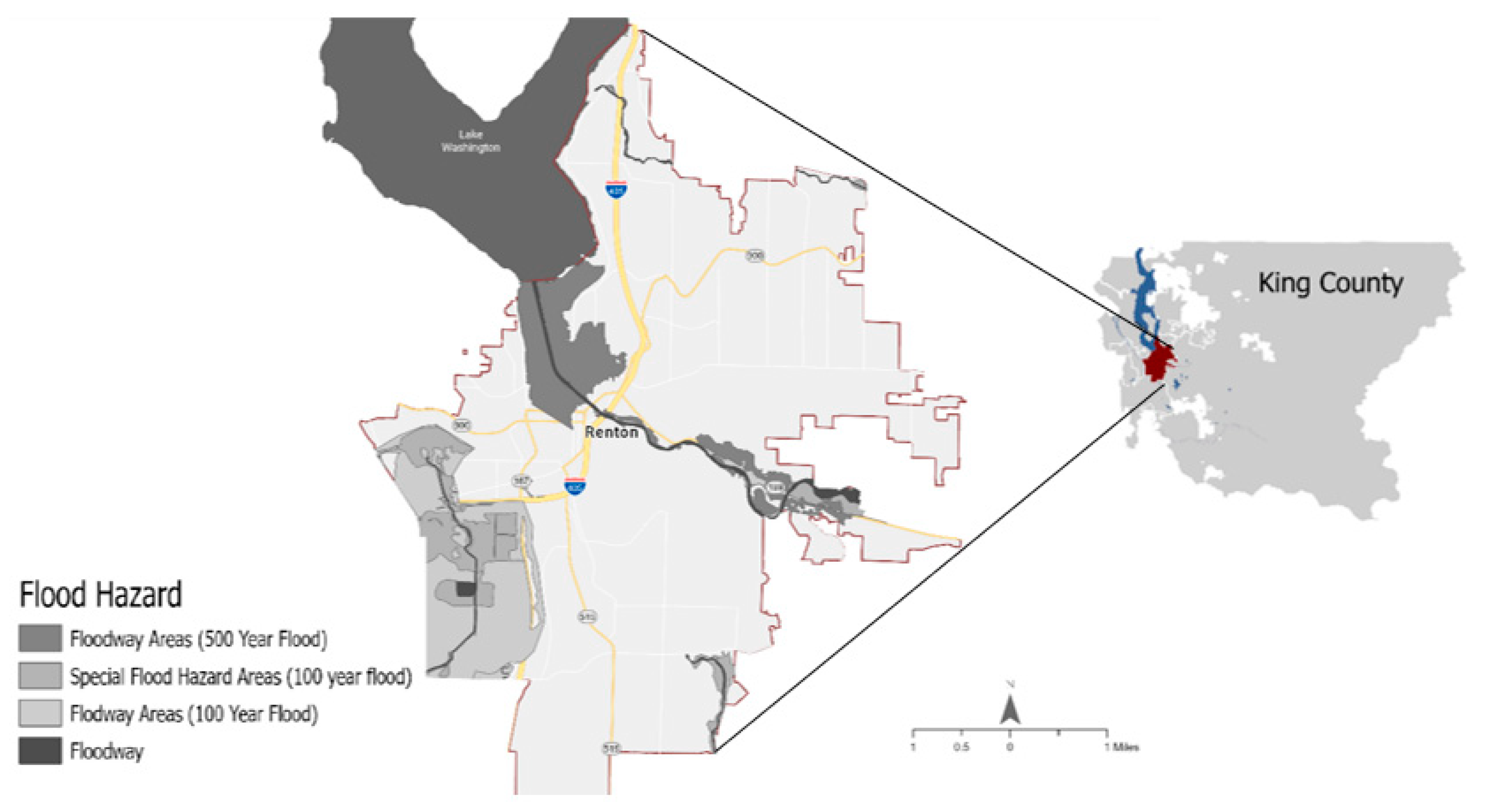
The study area is located in the city of Renton, WA, USA, which is a suburb of Seattle and is part of the lower Cedar River and Puget River Basin (Figure 1). It occupies nearly 53.82 km2 of areas comprising 606 sub-catchments of undeveloped land (52%) and paved developed areas (48%). The eastern part of the study area mainly contains commercial buildings, while the western part is primarily commercial, multifamily, high-density residential, medium-density residential, low-density residential, grass, forest, and wetland areas. The boundary to the northwest is marked by a ridgetop connecting the city to Lake Washington. The Cedar River flows through the city and into Lake Washington, collecting most of the stormwater. The regional climate is classified as mild Pacific maritime and is greatly influenced by the Pacific Ocean. It receives approximately 46 inches (1168.4 mm) of annual precipitation, of which nearly two-thirds occurs during the winter season from October to March. During the winter months, the region is also affected by storm systems associated with mid-latitude cooled jet streams and low-level jet streams ahead of the cold front (also known as the atmospheric river), resulting in snow and severe storms.
Based on the Federal Emergency Management Agency (FEMA), the floodplain zones in the city are shown in Figure 1. The flood zone designation in the area is primarily Zone X (moderate flood hazard areas) and Zone AE (special flood hazard area), which were established based on 500-year and 100-year floodplain elevations, respectively [58]. The flood risks in the region are rising, with the Puget Sound region experiencing at least 16 federally declared flood-related disasters with significant flooding and closing of highways since 1990 [59,60] showed considerable change in the atmospheric rivers and increasingly severe storms in the region over the past 30 years (1980 to 2009). The recent major flood events include the November 2022 flood caused by a record-breaking 203.2 mm (8 in) of rainfall over 24 h and the February 2020 phase four (severe) flood caused by the fifth-highest daily rainfall (82 mm) and snowmelt on the mountain [59]. Many areas in the city are experiencing challenges in adequately and effectively managing the increasing stormwater and floods. The cost of the damages from these floods were in the tens of millions of dollars, with the 2020 flood alone costing the city over USD 27 million in damages and associated costs [61]. The region is expected to experience severe floods more frequently in the future because of climate change [62]. The sea-level rise in Puget Sound is also expected to increase the flooding risk in the area. According to [49], the region may witness a maximum sea-level rise of 0.4 feet (12.19 cm) by 2030 and 2.2 feet (67 cm) by 2100 under the SSP-585 high-emissions scenario.
The existing drainage systems mainly comprise underground pipes, catch basins, curbs, and gutters, which collect runoff throughout the stormshed and direct it to a detention wetland for retention and natural treatment. Failure in and overflow from the stormwater systems often cause the flooding of streets and private property. The city spends about USD 3.5 million each year to improve stormwater infrastructure and reduce flooding [63]. In 2007, the city of Renton adopted a FEMA-based comprehensive stormwater system improvement project to address current and future basement and street flooding by increasing the size of the culverts within the watershed. However, the upgraded culverts failed during the recent severe flooding. Moreover, there will be an approximately 26% increase in the total discharge in the future climate change scenario compared to the historical period in the area, which will further aggravate the flooding problems in the future [64].
2.2. Datasets
The base input data for the model and optimization include precipitation, watershed, and stormwater drainage data. The DEM and land-cover data with 0.5 m and 10 m resolutions, respectively, were obtained from the city of Renton. The topography in the study area is relatively flat, with an elevation range from 6 to 9 m. The catchment boundaries and sub-catchments were delineated using DEM. The land covers are predominantly impervious surfaces (48% with commercial buildings ranging from 2030 m2 to 12,140 m2) and woodland (12%). The rest are grasses, small deciduous trees, and bushes. The high-resolution Soil Survey Geographical Database (SSURGO 2.2), obtained from the National Resources Conservation Service (NRCS) Geospatial Database, was used. The dominant soil type in the study area is Woodinville silty loam (Wo), with traces of Newberg silty loam (Ng) and Puget silty clay loam (Pu). All three types of soils have slow runoff potential and have high water holding capacity. The sub-catchment parameters, including area, slope, and infiltration characteristics, depth of depression storage for impervious and pervious surfaces, percent zero (percentage of impervious area that has no depression storage), Manning’s n values for impervious and pervious surfaces, and internal routing variables were used to determine the curve numbers for rainfall–runoff modeling. The 15-min precipitation data from 1 January 1995, through 1 May 2014, was obtained from the city of Renton database (https://green2.kingcounty.gov/hydrology/GaugeMap.aspx). The daily precipitation projection for 2020–2050 under the shared socioeconomic pathway (SSP585) emission scenario was downscaled from two CMIP6 climate models, namely MIROC6 and CMCC-ESM2. The projected daily precipitation data were biased-corrected and converted to 15 min data using the SCS Type IA distribution. The 15 min historical and future precipitation data were then used to develop the intensity–duration–frequency (IDF) curves of the storms in our study area.
2.3. Optimization Framework
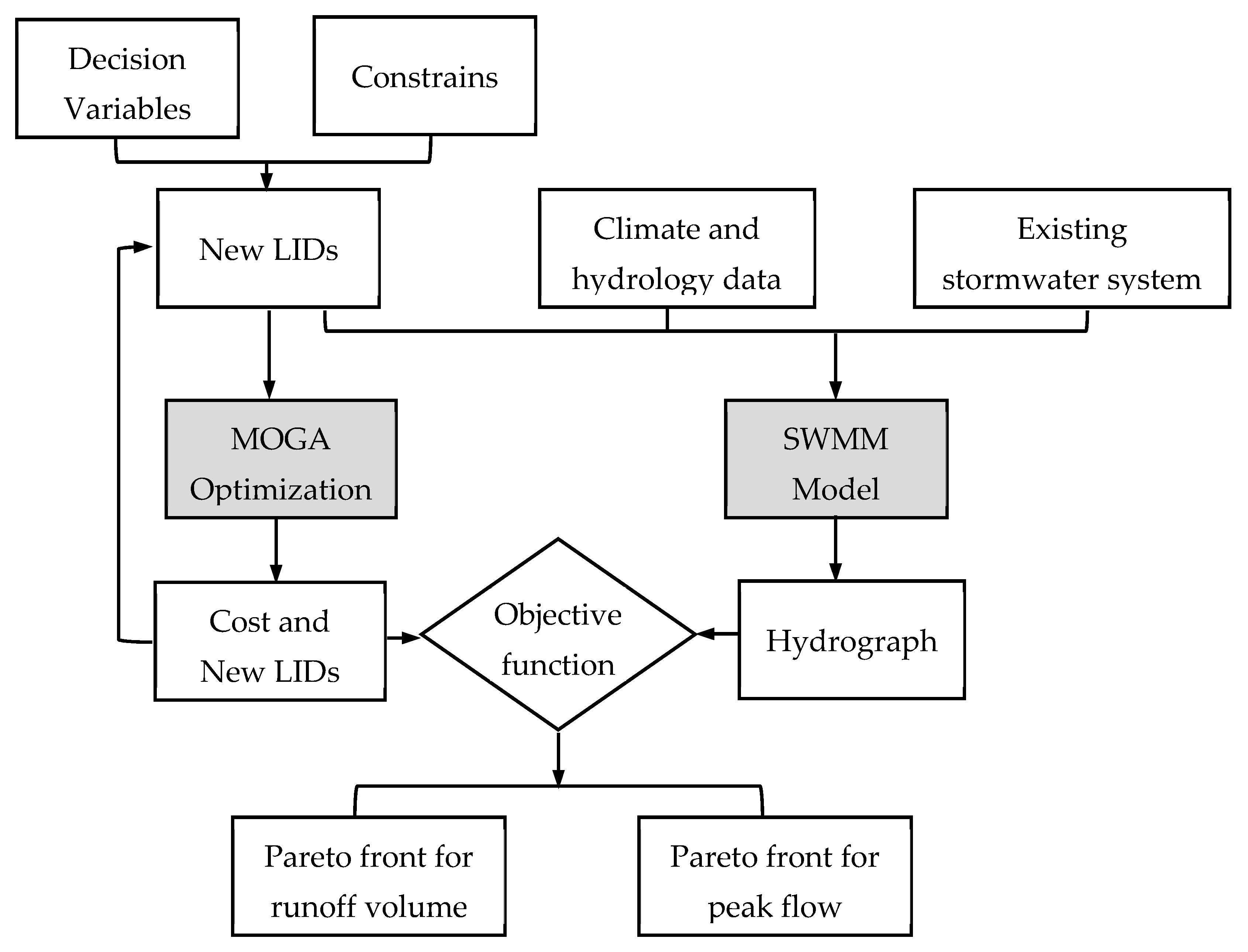
A simulation–optimization modeling framework (Figure 2) was developed to reduce total runoff and peak flow across the watershed at a minimum implementation cost of LIDs. The framework couples the SWMM model with a genetic algorithm (GA) to find Pareto optimal solutions for different LIDs and design parameters (i.e., type, number, location, and size). The Borg multi-objective evolutionary algorithm [32] was used because of its effectiveness in handling highly nonlinear problems and many decision variables.
The optimization framework was developed using MathWorks produces mathematical computing software MATLAB R2022b which is established in Las Vegas, USA to coupling the SWMM model and MOGA. The framework starts with a randomly generated initial population of LID type, size, location, and number, which are represented by binary strings of numbers or chromosomes in the MOGA. Each individual in the population is typically referred to as a chromosome and represents the size of a specific solution for the investigated problem. There are no lower or upper limits for population size. The SWMM then evaluates the performance of the individuals in the population based on the resultant runoff and cost. The simulation results from SWMM were sent back to the MOGA for constructing the Pareto-optimal front and generating the next generation. This process continues till optimized solutions are found, or user-specified limits are reached.
2.4. SWMM Model Development
The recent version of SWMM (5.1), which includes a toolbox to incorporate several LIDs, was used to simulate the stormwater runoff and evaluate the LIDs’ performances in reducing runoff at the basin outlet. The model effectively simulates the rainfall-runoff processes and the hydrodynamics associated with the stormwater system for both event-based and continuous rainfall events [48]. SWMM was also applied previously to optimize the LID implementations [45,65].
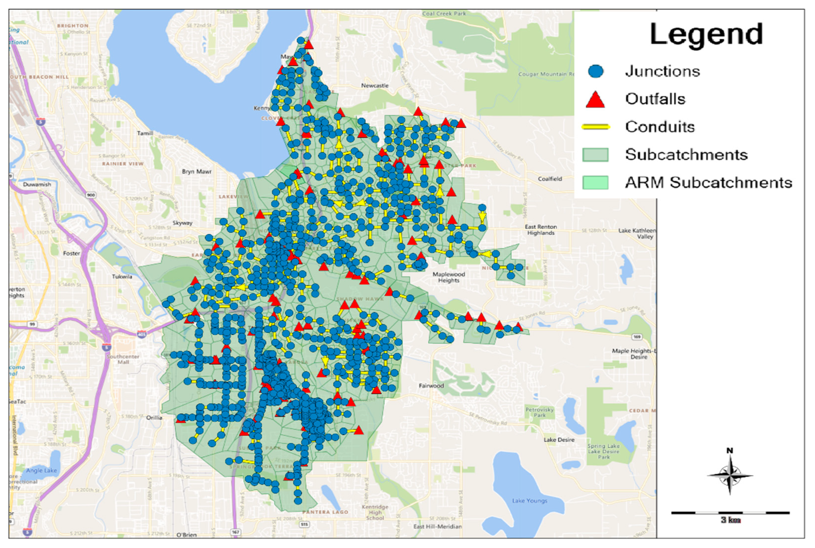
The study area was divided into 606 sub-catchments based on the topography (Figure 3). The sub-catchment area and average width were determined using the auto-length feature of SWMM as the backdrop technique and then scaling the dimensions. The sub-catchment width is important to calculate the overland flow distances that the flow travels before becoming channelized. The accuracy of the distances was confirmed by comparing with the topographical details of the stormshed. The slope and impervious areas were configured using GIS and the city of Renton’s geodatabase (CORMAP). The curve number method coupled with dynamic wave surface runoff routing and Manning channel routing was used to simulate the watershed runoff because of their computational efficiencies and previous applications for stormwater system optimization [7,66]. The dynamic wave routing method has the advantage of considering the backwater effects, channel storage, entrance/exit losses, pressurized flow, and flow reversal.
The existing stormwater system, including the LIDs, as well as proposed new LIDs, were incorporated into the model. The infiltration at the LIDs was computed using the Green-Ampt method that uses the initial moisture deficit, , parameter to represent the initial soil moisture condition before the storm. The initial values of were determined based on the soil types and the depth of the groundwater water table. The King County database (https://kingcounty.gov/services/gis/Maps/imap.aspx, during 20 June 2019 and 7 October 2019 was used to determine the groundwater level, which varies in depth from 0 to 16 feet. Given that the study area has predominately sandy loam soil type, we have considered initial moisture deficit values ranging from 0.35 for sand to 0.25 for sandy loam [66].
2.4.1. Sensitivity Analysis and Model Calibration
The SWMM model outputs can be sensitive to several input data and parameters, making sensitivity analysis an essential step in the model development [67]. Earlier studies found that time to peak and peak flows are significantly affected by the width of the sub-catchment and the soil moisture content [68]. In addition, the percent of imperviousness areas and slope of the catchment significantly influences flow hydrographs, particularly the peak flows. In this study, we considered different hydrological and catchment-related parameters such as percent zero imperv (or percent of the impervious area with no depression storage), percent of imperviousness, curve number, manning coefficient, and channel width for sensitivity analysis. The study area has negligible slopes; hence, the slope is not considered in the sensitivity analysis. Table 1 provides lists of parameters considered in the sensitivity test.
The SWMM model was manually calibrated using the sensitive sub-catchments and routing parameters. The initial values of the curve numbers and other variables (e.g., Manning’s n, storage depth) were identified from the sub-catchment characteristics and the SWMM manual [66]. The storm events from 18–20 June 2019 and 7 October 2019 were used to calibrate the SWMM model, while the storm events from 8 August 2019 and 8–9 October 2019 were used to validate the model. After the validation, the model was used to simulate the 50-year and 100-year past and future climate change scenario design storms with a 15 min time step. The high-emission scenario (SSP585) was used for a conservative design of LIDs and to assess their performance under a potential large increase in future storm intensity considered to generate the future storms.
2.4.2. Existing LID Types in Our Study
Five LIDs, namely the infiltration trench (IT), rain barrel (RB), rain garden (RG), bioretention (BR), and permeable pavement (PP), were used because of their current popularity in the study area. They were identified based on a literature review, locally available data, and consultation with an engineering company that has worked on municipal infrastructure projects in the area. The LIDs are often hydrologically designed as a series of vertical layers, and their properties are defined using per unit area. SWMM 5.1 performs water balance computations during the simulation to keep track of how much water is stored or moved within each LID layer. The LIDs parameters, including available area, land use, soil infiltration properties, water-table depth, and slope, were determined based on watershed characteristics and LID design standards. Table 2 shows the numbers of existing IT, RB, RG, BR, and PP in the study area and the estimated construction costs obtained from the city of Renton and online vendors.
2.4.3. Future Storm Considering Climate Change
The ability of LIDs to manage the expected increase in future climate-change scenario stormwater runoffs was assessed using the projected precipitations from the CMIP6 under SSP 585. The precipitation data from the CMIP6 have a coarse spatial resolution (ranging from 10 to 300 km) and are not suitable for direct use in the SWMM simulations. Therefore, the projected precipitation is commonly downscaled and bias corrected using statistical relationships with the observed precipitation [69]. Many statistical techniques are available to downscale and bias correct the projected precipitation, with the delta change (DC), quantile mapping (QM), and equidistance quantile mapping (EQM) methods being the most commonly used [70].
The DC method (Equation (1)) downscales and bias corrects the projected precipitation (2020–2050) by multiplying it with the ratio of observed and computed mean precipitations from the training period (1994–2014) [71].
where is the bias-corrected precipitation projection, is the precipitation projection from the climate models, and and are the means of observed and estimated precipitation from the climate models for the training period, respectively.
The DC method is easy to implement but is often limited in reproducing extreme precipitation because of its emphasis on the mean precipitation. In contrast, QM is capable of reproducing the full spectrum of the precipitation distribution as it corrects precipitations of different quantiles. However, the QM method is also limited because of its assumptions of constant variance and skewness of the climatic variables over the projection and training periods. This led to an extension of the QM method to EQM. The adjustment function (i.e., differences between observed and model values for any percentile during the training period) remains the same for the training and future periods in the QM method, whereas the EQM method also considers the differences between the cumulative distribution functions (CDFs) for the training and future periods. Mathematically, QM and EQM methods can be written as shown in Equations (2) and (3), respectively.
where and are the CDFs for the observed and predicted precipitation for the training period (1994–2014), respectively, and the biased corrected precipitation projections for 2020–2050.
We tested and compared the DC, QM, and EQM methods for downscaling the maximum daily precipitation. Two climate models (MIROC6 and CMCC-ESM2) from the CMIP6 were used because of their relatively good performances for the region. The Nash–Sutcliffe (NSE) and correlation coefficient (R2) are used to quantify the degree of agreement between observed and downscaled precipitation, with the value ranging between 0 and 1.
The downscaling approaches were further evaluated based on their performances to reproduce not only the mean precipitations but also the observed extreme precipitations. Frequency analysis of annual maximum daily precipitation was performed for the observed and downscaled precipitations. The results were compared to identify the best downscaling method, and the corresponding downscaled precipitation was used for developing the future IDF curves and design storms used for the SWMM simulations. For a particular return period, a typical IDF relationship can be described by a general mathematical statement provided in Equations (4)–(11).
where η are non-negative coefficients with ≤ 1. The equation was derived from the Sherman (1931) IDF equation:
where a is a function of the return period (T) and represents the quartile for the cumulative probability distribution associated with T. The denominator function b(d) can be expressed as:
where d is is the time duration (usually minutes), and θ and η are model parameters (θ > 0, 0 < η < 1).
a (T), which is ω in Equations (3)–(10), can be calculated using the following two empirical relations [72]:
where parameters λ and K depend on the return period T. a(T) is determined from the probability distribution function of the maximum rainfall intensity I(d) of a given duration d. The intensity of rainfall I(d) has a cumulative distribution of that is the same as the cumulative distribution of variable , which represents the rainfall intensity rescaled by . Mathematically, it can be expressed by:
where P is the cumulative probability calculated using:
Hence, or can be computed using:
Different cumulative distribution models are used to determine the .
Both the past and future data were used to construct the IDF curves. The future scenario for the annual maximum rainfalls for the years 2019–2049 with 1 h, 3 h, 6 h, 12 h, and 24 h durations were developed using the cumulative distribution functions (CDFs).
2.5. MOGA Optimization
The MOGA algorithm was used to optimize the implementation of new LIDs under the current and future storm conditions. The MOGA parameters are given in Table 3 and the description of the terms used is given in Supplementary Material Section S1. The optimization starts with an initial set of randomly generated N population (or chromosomes) made of genes representing the different values for the LIDs’ type, number, size, and location throughout the watershed. The decision variables were represented using binary encoding and decoding to facilitate data exchange between SWMM and MOGA. We used 10-bit chromosomes with 1024 (210) possible solutions as this avoids the duplicity of the solutions while providing sufficient variations to represent the decision variables. After the SWMM’s performance evaluation, crossover and mutation operators were applied to the initial population and generated the next population. First, better-performing individuals were identified as potential parents to produce offspring for the next generation. Then, some of the bites or genes in those individuals were randomly changed (mutated) before mixing them or applying crossover. Such selection and random gene changes ensure the survival of the fittest individuals and diversity that could lead to globally optimal solutions. Each chromosome bit was assigned a random real number ranging from 0.0 to 1.0. The mutation alters one more bit corresponding to the random numbers less than the specified mutation probability (0.001 to 0.05). In general, the mutation probability should be set to a low value, typically less than 0.5, to avoid the algorithm from switching to a random search. The optimization was done for four different design storms, representing the past (HIST 50 and HIST 100) and future (CC 50 and CC 100) design storms corresponding to the 50-year and 100-year return periods. The MOGA provides both the dominated and non-dominated solutions, which are used to develop the Pareto tradeoff between flow reduction and cost. The best solution from the Pareto front is identified as the point where there is a sudden change in the front, which is often known as the knee-of-curve point. This was done by estimating and comparing the slopes at each point on the Pareto front.
2.5.1. Implementation Strategies for New LIDs
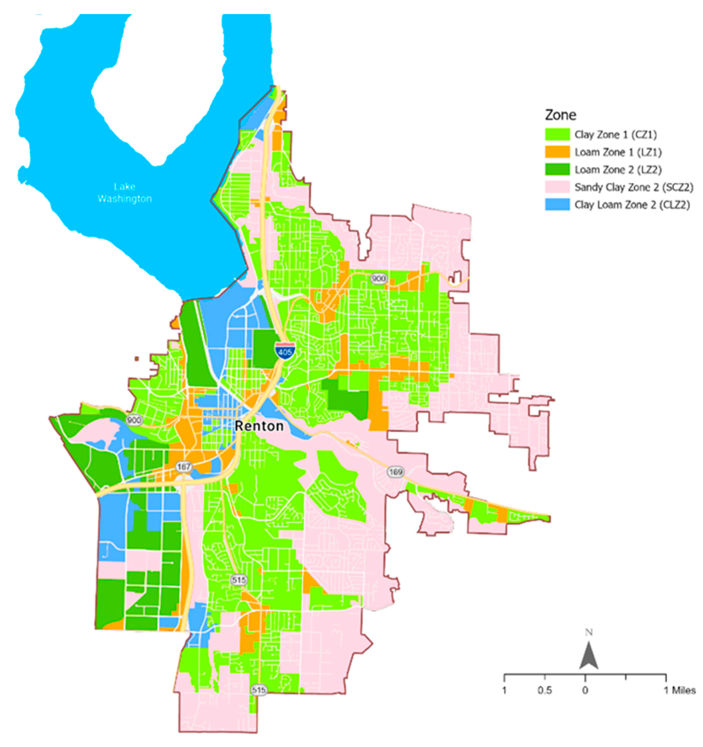
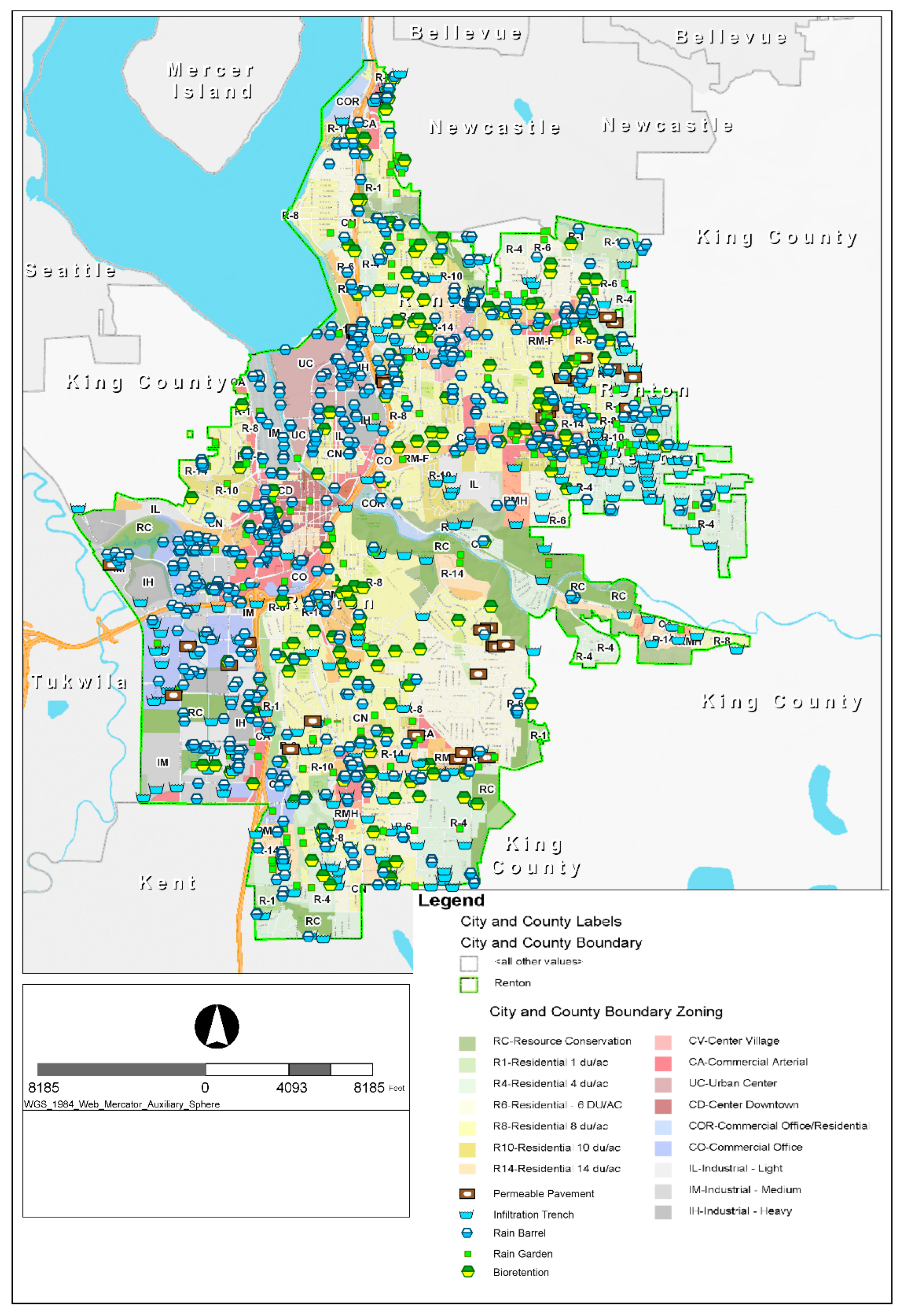
The implementation of new LIDs was determined based on the availability of spaces, which is expressed as the LID area ratio (or ratio of LID area and available open spaces in each sub-catchment). Current land cover categories (Figure 4) obtained from the city of Renton and King County include mostly commercial, multifamily, high density residential, medium density residential, low density residential, grass, forest, and wetland. Multifamily areas are defined by attached housing with greater than seven dwelling units per acre, high-density areas have four to seven dwelling units per acre, medium-density have one to three dwelling units per acre, and low-density have less than one dwelling unit per acre. The blocks in the sub-catchments were categorized into commercial and residential zones (Figure 5) to facilitate the LID implementations. The residential zones contain single-family areas, detached, and attached multi-units, covering 470 sub-catchments with a recommended runoff coefficient of 0.25–0.35. The residential zone was further categorized based on the soil type (Figure 4), as sandy and heavy soil with no crop, crop, pasture, and woodlands. The commercial zone, which covers 136 sub-catchments, consists of land use with a high percentage of impervious areas and runoff coefficient ranging from 0.70–0.95. The land cover and availability were used to constrain the choice of LIDs. For example, where there is not enough available land for LID expansion, RGs were chosen because of their minimum space requirements and low installation and maintenance costs. RBs were chosen for the private area as they take relatively smaller space but have higher costs of implementation. On the other hand, IT and BR are most suitable for sub-basins with parks and schools. The PP is a candidate to replace roads, sidewalks, and parking spaces in the industrial zone. In addition, the soil types were also used as constraints, with BR and IT recommended for area with sand, clay, and clay loam, while RG were considered for sites with 30% sandy soil and mixed with loamy topsoil to obtain proper drainage conditions.
The IT area ranges from 10 m2 to 300 m2 depending on the percentage of impervious area within a sub-watershed. They are typically implemented within 20% to 50% impervious area and can take up to 50% of the front yard and 50% of the driveway of private properties, while the width was considered to be between 1.0 and 1.5 m. RG was applied in areas with land slope below 4%, and its depth ranges from 75 mm to 150 mm based on the surface topography. The soil conditions also influence the RG sizes, with a poorly drained soil requiring a larger surface area with shallow depth, while a well-drained soil requires a smaller surface area with greater depth. The RG is considered to take 50% of the impervious runoff from driveways and 25% of the runoff from rooftops. The other 25% runoff from rooftops will be routed to RB, where there are 0 to 4 RB per house. Generally, the BR is more effective in areas with underlying clay or sandy soil.
The majority of the study area was considered moisture sensitive because of the dominant silt–loam soil and thicker topsoil in the area. During the wet season (October to March), an increase in soil moisture content can cause significant reduction in the infiltration capabilities. In addition, the wet soil dries at a slow rate, affecting the soil permeability. Thus, BR in our study area needs an underdrain at the bottom to allow more infiltration and drainage of the soil layers. PP (porous concrete and asphalt) were used for roads, private driveways, and parking lots. A commercial parking lot requires 7 cm thick permeable concrete pavers or 7–18 cm thick porous asphalt depending on vehicle types and runoff volume [73]. The storage and infiltration capability of PP generally depends on the number of LIDs per house and on the type of pavement. In general, 0 to 1 units of RG, BR, and PP were used per house. The different LIDs that currently exist in the study area and are used in the SWMM model are shown in Table S1. The potential locations of the different LIDs based on the above criteria (i.e., prior to the optimization) are shown in Figure 5.
Before optimizing the LID implementation, we tested the potential effectiveness of adding LIDs into the existing stormwater system and LIDs to reduce the historical and future climate-change scenario peak and total flow in the study area. We have conducted a preliminary study using six hypothetical LID scenarios, consisting of individual LIDs and combinations of different LIDs (Table 4).
2.5.2. Objective Functions
In general, the multi-objective function can be represented as follows:
where are the design variables and is the different objective functions. The multi-objective optimization problems can be minimizing or maximizing the above objective function and are solved iteratively by identifying sets of solutions comprised of the trade-off between the various objectives. In this study, we used three objective functions, including total flood volume and peak-flow discharge at the basin outlet, and construction costs of LIDs. The primary goal of the optimization process is to identify combinations of LIDs with variable sizes and locations that optimally decrease the total flow and peak flow at a minimal cost of construction. Mathematically, the three objective functions are given in Equations (13)–(15).
where represents the cost of LIDs type k per lot within sub-catchment j. This cost varies with the LID volume S and number N in the sub-catchment; n is total number of the different LIDs within the sub-catchment and m is the total number of sub-catchments. The average cost of each unit was estimated based on the standard cost presented in Table 2.
where and are the peak flow rate and flow volume, respectively, generated from the design storm from sub-catchment i. The total runoff volume is the sum of the volumes from each sub-catchment and over time.
2.5.3. Decision Variables
The decision variables include type, size, location, and number of LIDs. As described in Table 5, the implementation of these decision variables was constrained by soil type, land cover, available space, and other conditions. The list of decision variables, constraints, and feasible regions for number and sizes of LIDs are provided in Table S2. The feasible regions for the decision variables are defined as the sets of solutions that fulfill any constraints imposed on the variables [74].
3. Results and Discussions
3.1. Climate Change Impact on Future Storms
The observed and downscaled maximum daily precipitation from the MIROC6 and CMCC-ESM2 climate models are shown in Figure S1. Overall, the downscaled precipitation from the MIROC6 shows better performance compared to the CMCC-ESM2 in reproducing the observed precipitation. The MIROC6 has R2 and NSE values of 0.96 and 0.91, while CMCC-ESM2 has 0.91 and 0.77, respectively.
Additionally, Figure S2 compares the frequency analysis results for observed and downscaled annual maximum daily precipitation using the three downscaling methods for the MIROC6 and CMCC-ESM2 projections. The results show that in both cases the EQM method outperforms the other methods because of its ability to consider the different quantiles of the precipitation distribution separately during the bias correction. The delta method only considered the mean of the distribution and often underestimated the extreme precipitation. The MIROC6 also performs better than CMCC-ESM2, capturing the observed extreme precipitation.
The design storms, estimated from the IDF curves, are commonly used to design and manage stormwater systems. The 15-min precipitation data, collected from the city of Renton database (https://green2.kingcounty.gov/hydrology/GaugeMap.aspx, 1 January 1995 through 1 May 2014), was used to develop the historical IDF curves. The bias-corrected daily maximum precipitation from the MIROC6 model was converted to 15 min precipitation using the SCS Type IA distribution and used to develop the future IDF curves. Using these two datasets, the IDF curves for 2-, 5-, 10-, 20-, 50-, and 100-year return periods are constructed for both historical and future-scenario periods (Figure S3). The results show an increase (2.5% to 30%) in the storm intensities in the future scenario for all the return periods, with the increase being relatively more significant for higher return periods like the 50-year and 100-year storms.
3.2. Sensitivity Analysis
The detailed results of sensitivity analysis of SWMM are given in Table 5. In the present study, 5–15% perturbations in the sub-catchment’s width reduced the peak flow by 10.75–22.44%, whereas identical changes in CN reduced the peak flow from 17.29–24.74%. Sub-basins under consideration in this study have slopes within the shallow range. However, the slope parameter was not considered for the model calibration, but an increase in the depth of depression storage leads to a delayed flow after a storm event, minimizing total runoff and peak flows [69,71,73]. Zero percentage (impervious area with no depression storage) minimized the peak flow from 13.89–22.44% on 5–15% perturbance while the percent imperviousness decreased the peak flow by 15.25 to 23.51%. In this study, perturbations in CN indicated a significant impact on the peak flow while percent was the least sensitive parameter. Factoring other parameters under consideration, decreasing the catchment’s width leads to a reduction in peak flows, makes peaks less abrupt, and intensifies the hydrograph trailing arm. High variations in curve number magnitudes can be considered significant, similar to the effect of the percent imperviousness, while reduction in the percent width parameter effectively increases overland flow length and overland flow travel time.
3.3. Calibration and Validation of the SWMM Model
The SWMM model was calibrated and validated manually using the observed flow from four different rainfall events. Two rainfall events were used for manual calibration (Figure S4a,b), and the other two were used for validation of the model (Figure S4c,d). The calibration and validation resulted in good agreements between simulated and observed hydrographs, with NSE statistics ranging from 0.79 to 0.84 and R2 ranging from 0.81 to 0.87 for the four storms.
3.4. Potential of LID to Reduce Floods
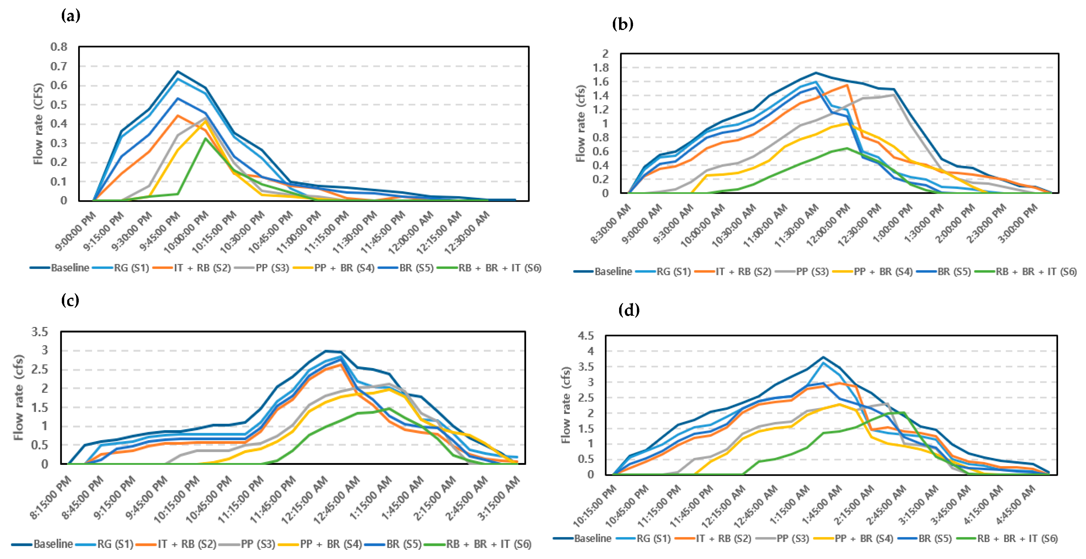
Prior to optimizing the LIDs, we tested their potential to reduce floods in our study area using six hypothetical LID implementation scenarios. Figure 6 shows the resulting hydrographs from the 50-year and 100-year design storms for the historical period (HIST 50 and HIST 100) and future-scenario period (CC 50 and CC100) compared with the baseline results that considered only the existing stormwater system. All the scenarios reduced the peak flows from historical and future-scenario storms. Overall, the peak flow and total runoff volume can be reduced by up to 13% and 29% under future climate-change scenarios and by up to 62% and 80% under the current storm conditions. Comparing the five individual LIDs, the infiltration trenches (IT) performed better in reducing the peak flow and runoff volume per construction cost, while the rain garden (RG) and bioretention (BR), respectively, are less effective in reducing the peak flows and total flow. The maximum reduction of runoff volume (80%) and peak flow (65%) were observed when a combination of rain barrel (RB), bioretention (BR), and infiltration trench (IT) was used (S6). The moderate performance of the bioretention (S5) was due to its small surface areas, causing overtop of stormwater when receiving a large portion of the surface water from the impervious area. The combination of infiltration trench and rain barrel (S2) provides a peak-flow hydrograph slightly lower than the individual LID under 50- and 100-year historical events. The peak discharge time for rain garden (S1), bioretention (S5), and mix of infiltration trench and rain barrel (S2) is nearly identical to the baseline scenario, while the other scenarios have delayed the peak discharge time.
3.5. Cost–Benefit Curves for Peak Flow
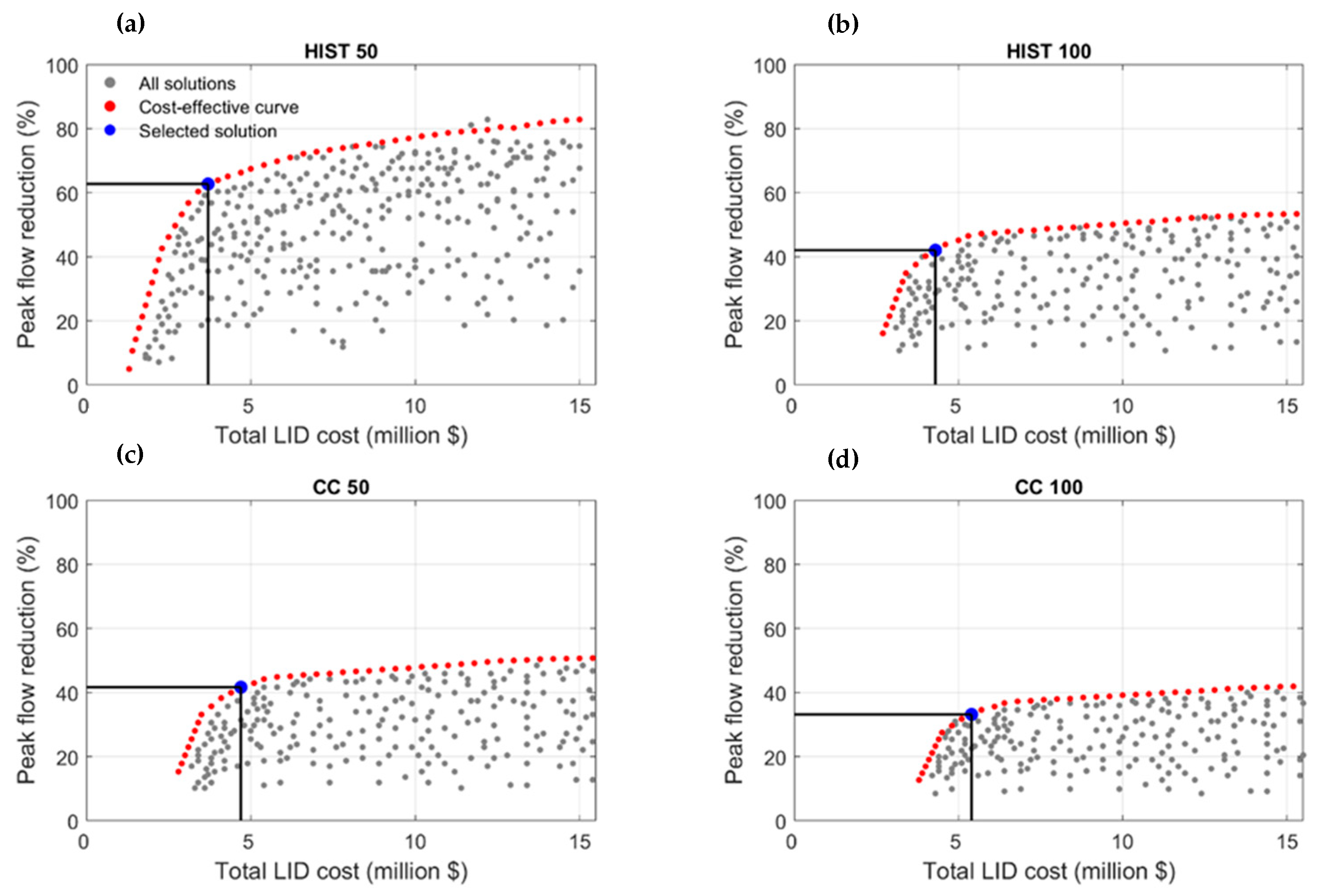
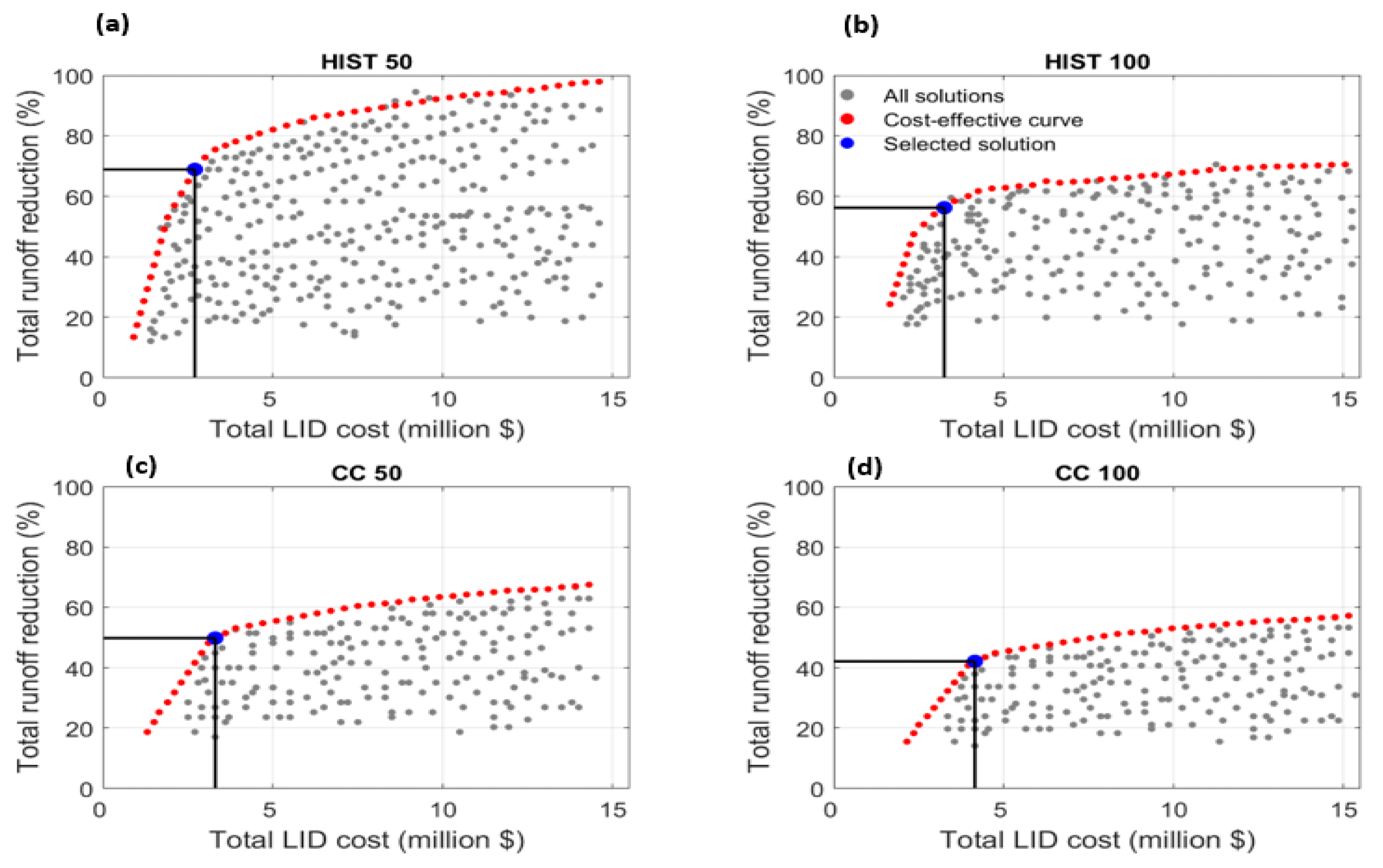
The multi-objective optimization provides optimal solutions and their potential trade-off for different objectives. In this study, the multi-objective consists of maximizing the peak flow and volume reduction and minimizing the construction cost of different LIDs. The performance of a given LID can vary depending on its size, number, and location. Figure 7 presents the optimal trade-offs (Pareto curves) between the percentage of peak-flow reduction and the construction costs under the historical and future climate scenarios. Each point in the figure represents a solution associated with an LID with a given size, number, and location. The red points represent the most cost-effective solutions. It has been found that the cost-effective curves generally show a significant increase in flow reduction with added investment on the LIDs up to a certain point, also known as knee of curve (blue dot), after which the LIDs’ performance does not improve considerably with the added investment. Therefore, the knee of curve is considered as the optimum solution. With an approximately USD 5 million investment on LIDs, the peak flows from past 50- and 100-year storms can be reduced by about 70% and 45%, while the peak flows from future-scenario 50- and 100-year storms can be reduced by about 42% and 35%, respectively. The additional investment beyond the USD 5 million will not significantly reduce the peak flows. Declining investment returns occur for investing beyond the effective solutions with the increase in the peak-flow reduction can only be obtained by investing in less efficient LIDs. The level of peak-flow reduction that can be achieved before a significant point of diminishing returns is reached depends on the limitations of the most efficient LID types in each scenario.
The results also show that the cost-effective solution varies with the storm sizes. For the HIST 50 storm, a 62.5% maximum reduction of peak flow was achieved with LID costing USD 3.9 million (Figure 7a). Whereas, for the HIST 100 storm, the maximum peak-flow reduction achieved was about 42% with a cost of USD 4.1 million (Figure 7b). These indicate that the LID practices performed differently for different design storms, and, as expected, flow reduction is higher for design storms with lower recurrence intervals (or moderate storms). For the future-scenario storms (CC100 and CC50), the peak flows are reduced by up to 33% and 42% at a total cost of USD 5.20 and USD 4.78 million, respectively (Figure 7c,d).
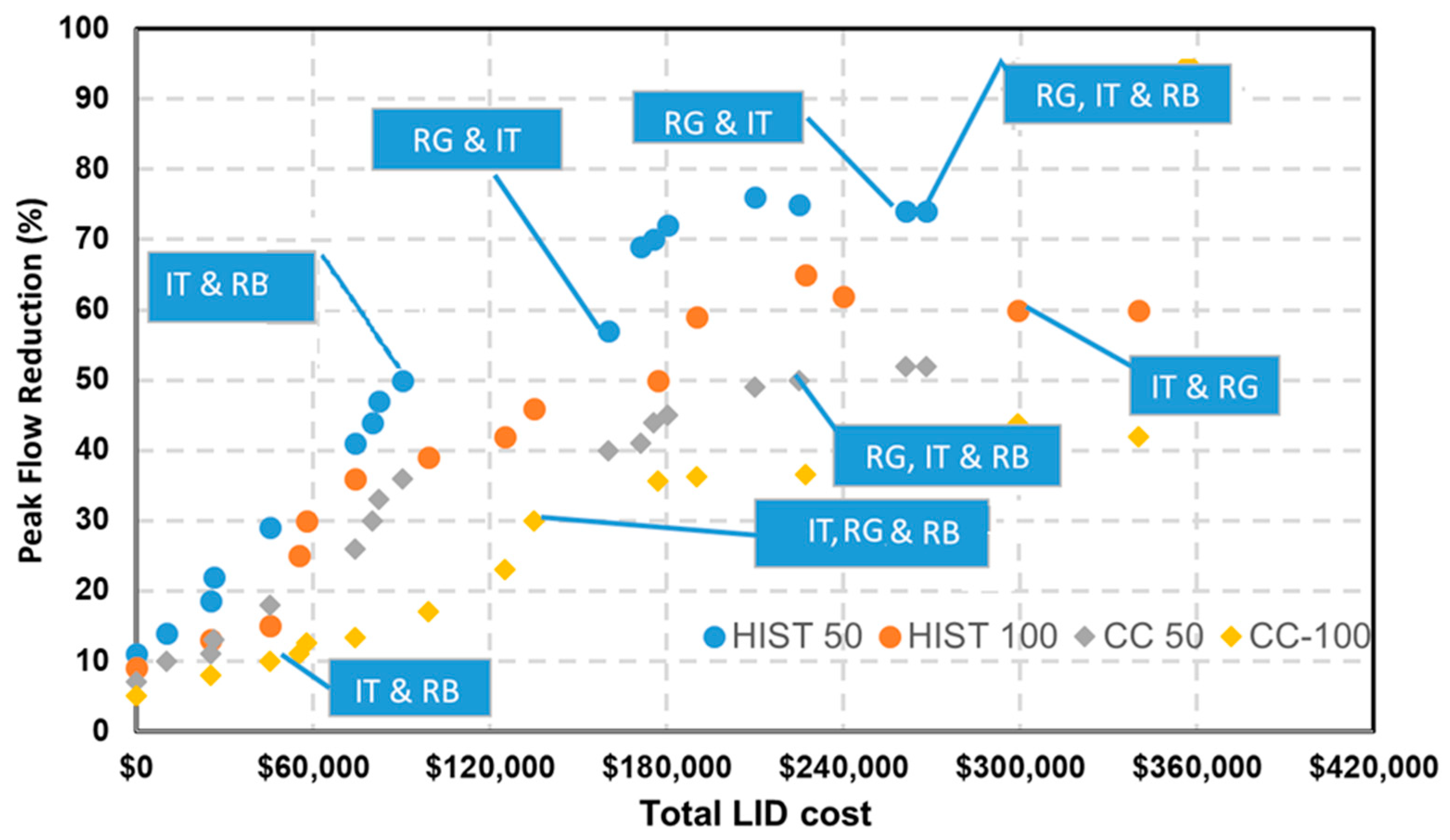
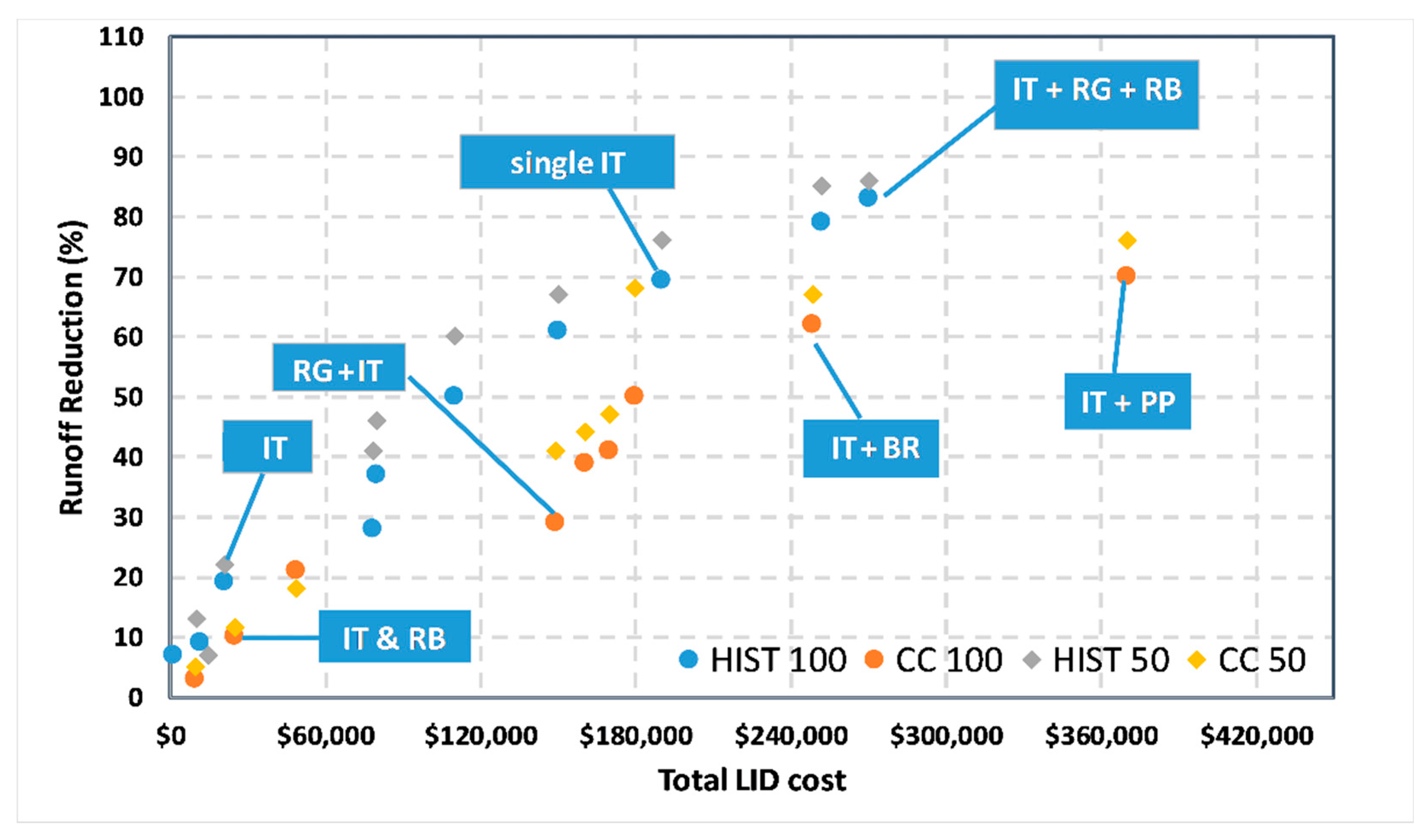
Figure 8 is breakdown to some of the LID mixes and decision variables contained in the cost-effective curves (red dots in Figure 7). The infiltration trench (IT) and its mix with other LIDs, such as rain gardens (RG), dominate the optimum solutions. The infiltration trenches (IT), with sizes ranging from 10 m2 to 300 m2 depending on the percentage of impervious land in the sub-catchment, are the most efficient and effective that can allow for further reduction of the peak flow by adding a rain garden (RG). Most trenches need continuously perforated pipes and relatively flat topography (slope < 1%). Higher slope reduces the infiltration and requires longer trenches at higher cost. Rain barrels (RB) are also present in some of the solutions but they are less effective at reducing peak flows than they are at reducing total runoff because they fill up before the most intense part of the precipitation event. Overall, a reduction of up to 50% peak flow from the past storm (HIST 50) was achieved with the use of IT and few RB that cost below USD 96,000. To further reduce the peak flow by up to 76%, the IT needs to be mixed with RG that costs about USD 269,000. The RB is relatively less effective in reducing peak flow from the future-scenario storm (CC-100) than HIST-50, achieving a maximum reduction of 30% with the related cost of USD 131,000. Although the combined uses of IT, RG, and RB provide high-flow reduction, they incur significantly high costs.
3.6. Cost–Benefit Curves for Total Runoff
The multi-objective solutions and the cost-effective curves for total runoff reduction are shown in Figure 9. The solutions are different from the peak-flow reduction solutions. Compared to the existing system, the optimized solutions for the HIST 50 and HIST 100 storms show a total runoff reduction of 70% and 58.2% with corresponding costs of USD 2.67 million and USD 3.5 million, respectively (Figure 9b,c). The reduction of total runoff for a CC 100 storm is around 6% lower than that of the CC 50, while the total cost is significantly increased because of the expected higher storm intensity for a CC 100 storm compared to the CC 50 storm.
The LIDs’ performances in reducing the total runoff were further evaluated using selected decision variables in Figure 10. The result shows that the increasing rate in cost-effective curves for the total flow reduction is steeper than that of the peak-flow reduction. This indicates that achieving a peak-flow reduction above the knee-of-curve point generally requires a higher cost than the total runoff reduction for all the four storm conditions we considered. In addition, the percentage reduction for total runoff for the identified LID practices is better overall than that of the peak runoff. Similar to the peak-flow result, the IT provides the most optimum cost–benefit solution for the total runoff reduction. Additionally, RB and RG are frequently found in a mix with IT to reduce the total runoff effectively. A higher reduction in flood volume was observed for infiltration trenches and permeable pavement (IT + PP) under the 100-year future-scenario storm, but they incur significantly increased costs (Figure 10).
In summary, based on the knee-of-curve results, it was observed that:
- Nearly 70% of the runoff volume from the 50-year past storm can be reduced using a combination of 30 ITs with a surface-area range of 4–80 m2, 70 RGs with a surface-area range of 4–10 m2, 18 BRs with a surface-area range of 4–10 m2, 9 PPs for driveways with a surface-area range of 20–80 m2, 100 RB with commercial size (200 L) at a total cost of USD 2.67 million;
- Approximately 58% of runoff volume from a 100-year past storm can be reduced using 79 ITs with a surface-area range of 10–80 m2, 77 RGs with a surface-area range of 8–10 m2, 12 PPs for driveways with a surface-area range of 20–80 m2, and 150 RBs with the commercial size 200–300 L at the cost of USD 3.5 million.
- Approximately 50% of runoff volume from a 50-year past storm can be reduced using 86 ITs with a surface-area range of 25–80 m2, 120 RGs with a surface-area range of 8–10 m2, 80 BRs with a surface-area range of 4–10 m2, 17 PPs for driveways with a surface-area range of 20–80 m2, 168 RBs with commercial size 200 L at the cost of USD 3.5 million dollars.
- The peak flows from the past 50-year and 100-year storms were decreased by 63% and 61%, with LIDs costing about USD 3.9 million and USD 4.3 million, respectively. Meanwhile, for the future-scenario 50-year and 100-year storms, the peak flow was reduced by 42% and 31% with USD 4.8 million and 5.2 million total costs, respectively.
4. Conclusions and Recommendations
The expansion of urban areas and increased extreme storms caused by climate change are causing severe floods to become more frequent in most regions. Many cities around the globe recognize the increasing trends in severe floods and have started upgrading the existing stormwater systems with relatively effective and sustainable LIDs. However, the effectiveness and cost of LIDs vary significantly depending on the characteristics of watersheds and design storms. For example, the widely used infiltration trench is only effective, both hydrologically and in cost, in areas where the topography has a gentle slope and the soil is deep with higher hydraulic conductivity. Thus, in most regions, mixing different LIDs and existing conventional stormwater systems and optimizing the size, location, and number of LIDS are essential to improve their performance and minimize cost.
The integrated SWMM–MOGA framework was first used to assess the performance of commonly used LIDs and then identify the hydrologically and cost-effective mixes of LIDS under both past- and future-scenario storm conditions in Renton City, WA. After confirming the benefit of adding LIDs to the existing stormwater system, we have optimized their applications by considering their sizes, locations, numbers, and watershed conditions. The reduction in peak flow, total runoff volume, and construction costs were used as objective functions for the optimization.
The results indicated that incorporating LIDs can significantly reduce the peak flow and total runoff in our study area. Overall, they appeared to be more effective in reducing total runoff than the peak flows, with the total runoff and peak-flow reductions ranging from 42% to 70% and 33% to 62.5% for the future 100-year and past 50-year storms, respectively. Combined uses of rain barrels, bioretention, and infiltration trenches represent the most effective LIDs to reduce the peak flow and volume in our study area. The effectiveness of a given type of LID is nonlinearly related to its design parameters, the combination of different LID practices, and storm magnitudes. For example, the optimized solution for the 100-year future storm indicated that a 50% runoff reduction (or 1200 m3) can be achieved with an implementation cost of USD 91,500. It costs three times more (USD 341,000) to further reduce the runoff by 2400 m3 from the same storm event.
The simulation–optimization framework from the study can be a useful decision-making tool to quantify the hydrological- and cost-effectiveness of different LIDs. It can assess the effect of different LIDs’ design parameters (e.g., placement and sizing of LIDs) on their performance and optimize the integrated LID and traditional stormwater system under different storm and urban development scenarios. Such a modeling framework allows the identification of an optimal LID implementation strategy for adapting to future climate change and providing quantitative information for urban planners, stormwater engineers, decision-makers, and stakeholders to implement an efficient and sustainable stormwater management system.
5. Limitations and Future Aspects
The presented study considered only a few popular LIDs in our study area. Including the other less commonly used LIDs (detention vaults and ponds) from the current stormwater system may further improve the overall performance. The water-quality benefits of the LIDs were not investigated in this study. Including water quality in the future-scenario study will give the decision-makers complete cost–benefit information on their investment in LIDs. In addition, when groundwater interferes with the LIDs because of a shallow water table, the model (which assumes conditions favorable to stormwater infiltration at LID sites) provides a poor simulation of the actual field conditions. This issue can be addressed to some level by adding an impervious layer underneath the LIDs to limit the infiltration. In addition, improving the modeling framework to account for the different sources of uncertainty will enhance its use as a decision-making tool. In modeling the future scenario, we only considered changes in storm events while considering the same land cover and static performance by LIDs. However, the continuously growing urban areas will impact the land cover by expanding the impervious surface. The current version of the framework does not explicitly account for the potential uncertainty in the climate projections. However, the framework can be run under different climate projections, representing the uncertainty range, to generate alternative implementations of LIDs. Finally, the study did not consider the flood risk caused by a sea-level rise since such a flood risk is relatively low in the city.
Supplementary Materials
The following supporting information can be downloaded at: https://www.mdpi.com/article/10.3390/w14193017/s1, Figure S1: Observed and biased-corrected daily precipitation from the (a) MIROC6 and (b) CMCC-ESM2 models.; Figure S2: The intensity-duration-frequency IDF curves for observed and downscaled annual maximum daily precipitation using different downscaling methods for the MIROC6 and CMCC-ESM2 GCMs; Figure S3: IDF curves for the historical (a) and future scenario (b) periods for the selected station; Figure S4: Graphs showings the flow rate Calibration period (a) 18–20 June 2019, (b) 7 October 2019 and Validation Periods (c) 8 October 2019 and (d) 21 August 2021; Table S1: The different LIDs and soil zones used in the SWMM model; Table S2: Decision variables and their feasible ranges.
Author Contributions
The two authors planned and designed the methods to study and optimize of Low Impact Development for sustainable stormwater management in a changing climate in the City of Renton, WA. Y.A. developed the model, calibrated and performed scenario analysis using SWMM model with included the climate change scenarios and analyzed the spatial scenario output data. Y.A. also prepared the tables and figures for the publication, wrote the text and formatted the paper. Y.D. guided and supervised the whole process, discussed results during the modeling study, and edited the manuscript. All authors have read and agreed to the published version of the manuscript.
Funding
This study was partly supported by the Department of Defense’s Strategic Environmental Research and Development Program (SERDP) under contact W912HQ15C0023.
Data Availability Statement
Data analyzed in this study are supported by King County and the city of Renton, WA, and are openly available in the following public domain resources: https://green2.kingcounty.gov/hydrology/GaugeMap.aspx (accessed on 26 November 2021).
Acknowledgments
The authors would like to thank the King County and city of Renton for all the data and material provided for this research.
Conflicts of Interest
The authors declare no conflict of interest.
Details of Nomenclature Used in This Study
| IT | Infiltration trench |
| RP | Rain barrel |
| RG | Rain garden |
| BR | Bioretention unit |
| PP | Permeable pavement |
| ITSCZ1 | Infiltration Trench-Sandy Clay-Zone One |
| ITSCZ2 | Infiltration Trench-Sandy Clay-Zone Two |
| ITLZ1 | Infiltration Trench-Loam-Zone One |
| ITLZ2 | Infiltration Trench-Loam-Zone Two |
| RBZ1 | Rain Barrel Zone One |
| RBZ2 | Rain Barrel Zone Two |
| RGSZ1 | Rain Garden-Sand-Zone One |
| RGCLZ2 | Rain Garden-Clay Loam-Zone Two |
| BRLZ2 | Bioretention-Loam-Zone Two |
| BRCSZ2 | Bioretention-Clay Sand-Zone Two |
| PPZ1 | Preamble Pavement Zone One |
| PPZ2 | Permeable Pavement Zone Two |
References
- Davis, A.P.; McCuen, R.H. Stormwater Management for Smart Growth; Springer: Berlin/Heidelberg, Germany, 2005; ISBN 038726048X. [Google Scholar]
- Kayhanian, M.; Fruchtman, B.D.; Gulliver, J.S.; Montanaro, C.; Ranieri, E.; Wuertz, S. Review of highway runoff characteristics: Comparative analysis and universal implications. Water Res. 2012, 46, 6609–6624. [Google Scholar] [CrossRef] [PubMed]
- Kaushal, S.S.; Belt, K.T. The urban watershed continuum: Evolving spatial and temporal dimensions. Urban Ecosyst. 2012, 15, 409–435. [Google Scholar] [CrossRef]
- Martin-Mikle, C.J.; de Beurs, K.M.; Julian, J.P.; Mayer, P.M. Identifying priority sites for low impact development (LID) in a mixed-use watershed. Landsc. Urban Plan. 2015, 140, 29–41. [Google Scholar] [CrossRef]
- Todeschini, S. Hydrologic and Environmental Impacts of Imperviousness in an Industrial Catchment of Northern Italy. J. Hydrol. Eng. 2016, 21, 05016013. [Google Scholar] [CrossRef]
- Chui, T.F.M.; Liu, X.; Zhan, W. Assessing cost-effectiveness of specific LID practice designs in response to large storm events. J. Hydrol. 2016, 533, 353–364. [Google Scholar] [CrossRef]
- Arjenaki, M.O.; Sanayei, H.R.Z.; Heidarzadeh, H.; Mahabadi, N.A. Modeling and investigating the effect of the LID methods on collection network of urban runoff using the SWMM model (case study: Shahrekord City). Model. Earth Syst. Environ. 2021, 7, 1–16. [Google Scholar] [CrossRef]
- Stovin, V.R.; Moore, S.L.; Wall, M.; Ashley, R.M. The potential to retrofit sustainable drainage systems to address combined sewer overflow discharges in the Thames Tideway catchment. Water Environ. J. 2013, 27, 216–228. [Google Scholar] [CrossRef]
- Duan, H.-F.; Li, F.; Yan, H. Multi-Objective Optimal Design of Detention Tanks in the Urban Stormwater Drainage System: LID Implementation and Analysis. Water Resour. Manag. 2016, 30, 4635–4648. [Google Scholar] [CrossRef]
- Visitacion, B.J.; Booth, D.B.; Steinemann, A.C. Costs and Benefits of Storm-Water Management: Case Study of the Puget Sound Region. J. Urban Plan. Dev. 2009, 135, 150–158. [Google Scholar] [CrossRef]
- Wang, M.; Zhang, D.; Adhityan, A.; Ng, W.J.; Dong, J.; Tan, S.K. Assessing cost-effectiveness of bioretention on stormwater in response to climate change and urbanization for future scenarios. J. Hydrol. 2016, 543, 423–432. [Google Scholar] [CrossRef]
- Barbosa, A.E.; Fernandes, J.N.; David, L.M. Key issues for sustainable urban stormwater management. Water Res. 2012, 46, 6787–6798. [Google Scholar] [CrossRef] [PubMed]
- Park, S.Y.; Lee, K.W.; Park, I.H.; Ha, S.R. Effect of the aggregation level of surface runoff fields and sewer network for a SWMM simulation. Desalination 2008, 226, 328–337. [Google Scholar] [CrossRef]
- Li, C.; Fletcher, T.D.; Duncan, H.P.; Burns, M.J. Can stormwater control measures restore altered urban flow regimes at the catchment scale? J. Hydrol. 2017, 549, 631–653. [Google Scholar] [CrossRef]
- Ahiablame, L.M.; Engel, B.A.; Chaubey, I. Effectiveness of Low Impact Development Practices: Literature Review and Suggestions for Future Research. Water Air Soil Pollut. 2012, 223, 4253–4273. [Google Scholar] [CrossRef]
- Randhir, T.O.; Raposa, S. Urbanization and watershed sustainability: Collaborative simulation modeling of future development states. J. Hydrol. 2014, 519, 1526–1536. [Google Scholar] [CrossRef]
- Gu, C.; Cockerill, K.; Anderson, W.P.; Shepherd, F.; Groothuis, P.A.; Mohr, T.M.; Whitehead, J.C.; Russo, A.A.; Zhang, C. Modeling effects of low impact development on road salt transport at watershed scale. J. Hydrol. 2019, 574, 1164–1175. [Google Scholar] [CrossRef]
- Dietz, M.E. Low Impact Development Practices: A Review of Current Research and Recommendations for Future Directions. Water. Air. Soil Pollut. 2007, 186, 351–363. [Google Scholar] [CrossRef]
- Seo, M.; Jaber, F.; Srinivasan, R.; Jeong, J. Evaluating the Impact of Low Impact Development (LID) Practices on Water Quantity and Quality under Different Development Designs Using SWAT. Water 2017, 9, 193. [Google Scholar] [CrossRef]
- Jackisch, N.; Weiler, M. The hydrologic outcome of a Low Impact Development (LID) site including superposition with streamflow peaks. Urban Water J. 2017, 14, 143–159. [Google Scholar] [CrossRef]
- Tredway, J.C.; Havlick, D.G. Assessing the Potential of Low-Impact Development Techniques on Runoff and Streamflow in the Templeton Gap Watershed, Colorado. Prof. Geogr. 2017, 69, 372–382. [Google Scholar] [CrossRef]
- Sohn, W.; Kim, J.-H.; Li, M.-H.; Brown, R. The influence of climate on the effectiveness of low impact development: A systematic review. J. Environ. Manag. 2019, 236, 365–379. [Google Scholar] [CrossRef] [PubMed]
- Wu, X.; Lu, Y.; Zhou, S.; Chen, L.; Xu, B. Impact of climate change on human infectious diseases: Empirical evidence and human adaptation. Environ. Int. 2016, 86, 14–23. [Google Scholar] [CrossRef]
- Zhan, W.; Chui, T.F.M. Evaluating the life cycle net benefit of low impact development in a city. Urban For. Urban Green. 2016, 20, 295–304. [Google Scholar] [CrossRef]
- Hu, M.; Sayama, T.; Zhang, X.; Tanaka, K.; Takara, K.; Yang, H. Evaluation of low impact development approach for mitigating flood inundation at a watershed scale in China. J. Environ. Manag. 2017, 193, 430–438. [Google Scholar] [CrossRef] [PubMed]
- Seo, M.; Jaber, F.; Srinivasan, R. Evaluating Various Low-Impact Development Scenarios for Optimal Design Criteria Development. Water 2017, 9, 270. [Google Scholar] [CrossRef]
- Cook, P.G.; Wood, C.; White, T.; Simmons, C.T.; Fass, T.; Brunner, P. Groundwater inflow to a shallow, poorly-mixed wetland estimated from a mass balance of radon. J. Hydrol. 2008, 354, 213–226. [Google Scholar] [CrossRef]
- United States Environmental Protection Agency (USEPA). National Water Quality Inventory. Available online: http://www.epa.gov/sites/production/files/201509/documents/2000_national_water_quality_inventory_report_to_congress.pdf (accessed on 15 October 2020).
- Williams, E.S.; Wise, W.R. Hydrologic Impacts of Alternative Approaches to Storm Water Management and Land Development1. J. Am. Water Resour. Assoc. 2006, 42, 443–455. [Google Scholar] [CrossRef]
- Gallo, C.; Moore, A.; Wywrot, J. Comparing the Adaptability of Infiltration Based Bmps to Various U.S. Regions. Landsc. Urban Plan. 2012, 106, 326–335. [Google Scholar] [CrossRef]
- Giacomoni, M.H.; Joseph, J. Multi-Objective Evolutionary Optimization and Monte Carlo Simulation for Placement of Low Impact Development in the Catchment Scale. J. Water Resour. Plan. Manag. 2017, 143. [Google Scholar] [CrossRef]
- Zhang, G.; Hamlett, J.M.; Reed, P.; Tang, Y. Multi-Objective Optimization of Low Impact Development Designs in an Urbanizing Watershed. Open J. Optim. 2013, 2, 95–108. [Google Scholar] [CrossRef] [Green Version]
- Eckart, K.; McPhee, Z.; Bolisetti, T. Multiobjective optimization of low impact development stormwater controls. J. Hydrol. 2018, 562, 564–576. [Google Scholar] [CrossRef]
- Alfredo, K.; Montalto, F.; Goldstein, A. Observed and Modeled Performances of Prototype Green Roof Test Plots Subjected to Simulated Low- and High-Intensity Precipitations in a Laboratory Experiment. J. Hydrol. Eng. 2010, 15, 444–457. [Google Scholar] [CrossRef]
- Oberascher, M.; Zischg, J.; Palermo, S.A.; Kinzel, C.; Rauch, W.; Sitzenfrei, R. Smart Rain Barrels: Advanced Lid Management through Measurement and Control. In New Trends in Urban Drainage Modelling. Udm 2018. Green Energy and Technology; Mannina, G., Ed.; Springer: Copenhagen, Denmark, 2019; pp. 777–782. ISBN 978-3-319-99866-4. [Google Scholar]
- Qin, H.; Li, Z.; Fu, G. The effects of low impact development on urban flooding under different rainfall characteristics. J. Environ. Manag. 2013, 129, 577–585. [Google Scholar] [CrossRef] [PubMed]
- Eckart, K.; McPhee, Z.; Bolisetti, T. Performance and implementation of low impact development–A review. Sci. Total Environ. 2017, 607–608, 413–432. [Google Scholar] [CrossRef] [PubMed]
- Zhu, Z.; Chen, X. Evaluating the Effects of Low Impact Development Practices on Urban Flooding under Different Rainfall Intensities. Water 2017, 9, 548. [Google Scholar] [CrossRef]
- Sahana, M.; Hong, H.; Sajjad, H. Analyzing urban spatial patterns and trend of urban growth using urban sprawl matrix: A study on Kolkata urban agglomeration, India. Sci. Total Environ. 2018, 628–629, 1557–1566. [Google Scholar] [CrossRef]
- Leimgruber, J.; Krebs, G.; Camhy, D.; Muschalla, D. Model-Based Selection of Cost-Effective Low Impact Development Strategies to Control Water Balance. Sustainability 2019, 11, 2440. [Google Scholar] [CrossRef]
- Liu, Y.; Theller, L.O.; Pijanowski, B.C.; Engel, B.A. Optimal selection and placement of green infrastructure to reduce impacts of land use change and climate change on hydrology and water quality: An application to the Trail Creek Watershed, Indiana. Sci. Total Environ. 2016, 553, 149–163. [Google Scholar] [CrossRef]
- Elliott, A.; Trowsdale, S. A review of models for low impact urban stormwater drainage. Environ. Model. Softw. 2007, 22, 394–405. [Google Scholar] [CrossRef]
- Trinh, D.H.; Chui, T.F.M. Assessing the hydrologic restoration of an urbanized area via an integrated distributed hydrological model. Hydrol. Earth Syst. Sci. 2013, 17, 4789–4801. [Google Scholar] [CrossRef] [Green Version]
- Morsy, M.M.; Goodall, J.L.; Shatnawi, F.M.; Meadows, M.E. Distributed Stormwater Controls for Flood Mitigation within Urbanized Watersheds: Case Study of Rocky Branch Watershed in Columbia, South Carolina. J. Hydrol. Eng. 2016, 21, 11. [Google Scholar] [CrossRef]
- Goncalves, M.; Zischg, J.; Rau, S.; Sitzmann, M.; Rauch, W.; Kleidorfer, M. Modeling the Effects of Introducing Low Impact Development in a Tropical City: A Case Study from Joinville, Brazil. Sustainability 2018, 10, 728. [Google Scholar] [CrossRef]
- Bach, P.M.; Rauch, W.; Mikkelsen, P.S.; McCarthy, D.T.; Deletic, A. A critical review of integrated urban water modelling–Urban drainage and beyond. Environ. Model. Softw. 2014, 54, 88–107. [Google Scholar] [CrossRef]
- Lerer, S.; Arnbjerg-Nielsen, K.; Mikkelsen, P. A Mapping of Tools for Informing Water Sensitive Urban Design Planning Decisions—Questions, Aspects and Context Sensitivity. Water 2015, 7, 993–1012. [Google Scholar] [CrossRef]
- Rossman, L.A.; Epa, U. Modeling Low Impact Development Alternatives with SWMM. J. Water Manag. Model. 2010, 11, 167–182. [Google Scholar] [CrossRef]
- Denault, C.; Millar, R.G.; Lence, B.J. Assessment of Possible Impacts of Climate Change in an Urban Catchment. J. Am. Water Resour. Assoc. 2006, 42, 685–697. [Google Scholar] [CrossRef]
- Zahmatkesh, Z.; Karamouz, M.; Goharian, E.; Burian, S.J. Analysis of the Effects of Climate Change on Urban Storm Water Runoff Using Statistically Downscaled Precipitation Data and a Change Factor Approach. J. Hydrol. Eng. 2015, 20, 05014022. [Google Scholar] [CrossRef]
- Zhen, X.-Y.; Yu, S.L.; Lin, J.-Y. Optimal Location and Sizing of Stormwater Basins at Watershed Scale. J. Water Resour. Plan. Manag. 2004, 130, 339–347. [Google Scholar] [CrossRef]
- Maringanti, C.; Chaubey, I.; Arabi, M. A multi-objective optimization tool for the selection and placement of BMPs for pesticide control. Hydrol. Earth Syst. Sci. Discuss. 2008, 5, 1821–1862. [Google Scholar] [CrossRef]
- Liang, L.; Gong, P. Climate change and human infectious diseases: A synthesis of research findings from global and spatio-temporal perspectives. Environ. Int. 2017, 103, 99–108. [Google Scholar] [CrossRef]
- Ghodsi, S.H.; Zahmatkesh, Z.; Goharian, E.; Kerachian, R.; Zhu, Z. Optimal design of low impact development practices in response to climate change. J. Hydrol. 2020, 580, 124266. [Google Scholar] [CrossRef]
- Wu, J.; Yang, R.; Song, J. Effectiveness of Low-Impact Development for Urban Inundation Risk Mitigation under Different Scenarios: A Case Study in Shenzhen, China. Nat. Hazards Earth Syst. Sci. 2018, 18, 2525–2536. [Google Scholar] [CrossRef]
- Xu, T.; Jia, H.; Wang, Z.; Mao, X.; Xu, C. SWMM-based methodology for block-scale LID-BMPs planning based on site-scale multi-objective optimization: A case study in Tianjin. Front. Environ. Sci. Eng. 2017, 11, 1. [Google Scholar] [CrossRef]
- Miller, G.; Tyler; Spoolman, S. Environmental Science; Cengage Learning: Boston, MA, USA, 2012. [Google Scholar]
- Beck, R.W. City of Renton Springbrook Creek FEMA Remapping Study, Activity 1-Field Surveys and Reconnaissance; R. W. Beck, Inc.: Renton, WA, USA, 2003. [Google Scholar]
- King County. 2020. Available online: https://your.kingcounty.gov/dnrp/library/water-andland/flooding/Flood-Brochures/2020-2021-flood-brochures/20-21-be-flood-ready-brochure-countywide.pdf (accessed on 10 December 2020).
- Neiman, P.J.; Schick, L.J.; Ralph, F.M.; Hughes, M.; Wick, G.A. Flooding in western Washington: The connection to atmospheric rivers. J. Hydrometeorol. 2011, 12, 1337–1358. [Google Scholar] [CrossRef]
- King County. Available online: https://kingcountyfloodcontrol.org/wp-content/uploads/2020/12/2019-2020-Flood-Season-Report-FINAL.pdf. (accessed on 10 May 2020).
- Scarborough, P.; Adhikari, V.; Harrington, R.A.; Elhussein, A.; Briggs, A.; Rayner, M.; Adams, J.; Cummins, S.; Penney, T.; White, M. Impact of the announcement and implementation of the UK soft drinks industry levy on sugar content, price, product size and number of available soft drinks in the UK, 2015–2019: A controlled interrupted time series analysis. PLoS Med. 2020, 17, e1003025. [Google Scholar] [CrossRef] [PubMed]
- SWDM. 2017. Available online: https://rentonwa.gov/UserFiles/Servers/Server_7922657/File/City%20Hall/Public%20Works/Utility%20Systems/Surface%20Water%20Design%20Standards/2017RentonSWDM_Complete_Final_Final.pdf (accessed on 10 October 2020).
- Abduljaleel, Y.; Demissie, Y. Evaluation and Optimization of Low Impact Development Designs for Sustainable Stormwater Management in a Changing Climate. Water 2021, 13, 2889. [Google Scholar] [CrossRef]
- Campisano, A.; Gnecco, I.; Modica, C.; Palla, A. Designing domestic rainwater harvesting systems under different climatic regimes in Italy. Water Sci. Technol. 2013, 67, 2511–2518. [Google Scholar] [CrossRef]
- Rossman, L.A. Storm Water Management Model User’s Manual, Version 5.0. Available online: https://www.owp.csus.edu/LIDTool/Content/PDF/SWMM5Manual.pdf (accessed on 10 December 2020).
- Iooss, B.; Lemaître, P. A review on global sensitivity analysis methods. In Uncertainty Management in Simulation-Optimization of Complex Systems; Springer: Boston, MA, USA, 2015; pp. 101–122. [Google Scholar]
- The City of Renton. 2019. Available online: https://kingcounty.gov/~/media/depts/emergency/management/documents/plans/hazard-mitigation/City_of_Renton_Annex.ashx?la=en (accessed on 1 November 2020).
- Ballinas-González, H.A.; Alcocer-Yamanaka, V.H.; Canto-Rios, J.J.; Simuta-Champo, R. Sensitivity Analysis of the Rainfall–Runoff Modeling Parameters in Data-Scarce Urban Catchment. Hydrology 2020, 7, 73. [Google Scholar] [CrossRef]
- Qian, W.; Chang, H.H. Projecting Health Impacts of Future Temperature: A Comparison of Quantile-Mapping Bias-Correction Methods. Int. J. Environ. Res. Public Health 2021, 18, 1992. [Google Scholar] [CrossRef]
- Dessu, S.B.; Melesse, A.M. Evaluation and Comparison of Satellite and Gcm Rainfall Estimates for the Mara River Basin, Kenya/Tanzania. In Climate Change and Water Resources; Younos, T., Grady, C.A., Eds.; Springer: Berlin/Heidelberg, Germany, 2013; pp. 29–45. ISBN 978-3-642-37585-9. [Google Scholar]
- Ven, C.; David, T.; Maidment, R.; Larry, W. Mays. In Applied Hydrology, International Edition; MacGraw-Hill, Inc.: New York, NY, USA, 1988; p. 149. [Google Scholar]
- Villarini, G.; Smith, J.A.; Serinaldi, F.; Ntelekos, A.A.; Schwarz, U. Analyses of extreme flooding in Austria over the period 1951–2006. Int. J. Climatol. 2012, 32, 1178–1192. [Google Scholar] [CrossRef]
- Deb, K. Multi-Objective Optimization Using Evolutionary Algorithms, 1st ed.; John Wiley & Sons: New York, NY, USA, 2001; ISBN 978-0-471-87339-6. [Google Scholar]
Figure 1.
The location and flood hazard map of the study area (Renton city), which is located in King County, WA, USA.
Figure 1.
The location and flood hazard map of the study area (Renton city), which is located in King County, WA, USA.

Figure 2.
The modeling framework, integrating SWMM and MOGA.

Figure 3.
The sub-catchments and existing stormwater system in our study area.

Figure 4.
Soil zones used to determine the suitability of locations for a given LID.

Figure 5.
Locations of the proposed LIDs and distributions of the soil types.

Figure 6.
Hydrographs for the implementation of LID practices scenarios for (a) HIST 50, (b) HIST 100, (c) CC 50, and (d) CC 100.
Figure 6.
Hydrographs for the implementation of LID practices scenarios for (a) HIST 50, (b) HIST 100, (c) CC 50, and (d) CC 100.

Figure 7.
The trade-off for peak flow reduction and cost of LIDs under past- (HIST 50, HIST 100) and future-scenario (CC 50, CC 100) storms.
Figure 7.
The trade-off for peak flow reduction and cost of LIDs under past- (HIST 50, HIST 100) and future-scenario (CC 50, CC 100) storms.

Figure 8.
Peak-flow reduction versus implementation costs for selected optimal design variables of LIDs.
Figure 8.
Peak-flow reduction versus implementation costs for selected optimal design variables of LIDs.

Figure 9.
Reduction of total runoff versus LID implementation costs under the four storm scenarios: (a) HIST 50, (b) HIST 100, (c) CC 50, and (d) CC 100.
Figure 9.
Reduction of total runoff versus LID implementation costs under the four storm scenarios: (a) HIST 50, (b) HIST 100, (c) CC 50, and (d) CC 100.

Figure 10.
Total runoff reduction and associated costs of LIDs for hist- and CC-storm scenarios.


Table 1.
SWMM parameters used for the sensitivity analysis.
| Parameters | Values | Initial Values Source |
|---|---|---|
| Sub-catchment width | Variable | Geometry |
| Manning’s n for impervious surface | 0.05–0.15 | SWMM manual |
| Impervious percentage with no depression (%) | 5–15 | SWMM manual |
| Curve number | Variable | DEM, land use, and soil data |
Table 2.
The five existing LIDs considered in our study, their associated costs, sizes, and implementation strategies.
Table 2.
The five existing LIDs considered in our study, their associated costs, sizes, and implementation strategies.
| LIDs | Cost in WA | No. LIDs | Implementation Strategies |
|---|---|---|---|
| Bioretention Cell (BR) | 4.8 USD/m2 | 78 | Bioretention (BR) captures runoff from sidewalk and 1/4 of driveway and parking lots in commercial development. |
| Rain Barrel (RB) | 150 USD/unit | 130 | Rain barrels (RB) collect water from the entire roof of a house. |
| Permeable Pavement (PP) | 30.16 USD/m2 | 43 | Permeable pavement captures runoff from the entire driveway and parking lot in commercial development. |
| Infiltration Trench (IT) | 3.36 USD/m2 | 90 | The infiltration trench (IT) captures runoff from half of the walkway along with the front houses and half of the driveway. |
| Rain Garden (RG) | 3 USD/m2 | 105 | Rain garden (RG) captures water from half of the house roof and half of the driveway. |
Table 3.
MOGA parameters used for the LIDs optimization.
| Parameter | Value |
|---|---|
| Initial population size | 100 |
| Maximum population size | 200 |
| Probability for crossover | 1 |
| Probability for mutation | 0.03 |
| Maximum generations per run | 25 |
| Maximum number of function evaluations | 10,000 |
Table 4.
Hypothetical LID scenarios to evaluate the effectiveness of redesigning the existing LIDs.
| Scenario | Description | |
|---|---|---|
| S1 | RG only | Use only rain garden (RG) to collect runoff from the houses. |
| S2 | IT + RB | Use infiltration trench (IT) and rain barrel (RB) to collect the runoff from roof and surrounding areas of houses. |
| S3 | PP | Use permeable pavement to collect runoff from commercial regions. |
| S4 | PP + BR | Use permeable pavement and bioretention (BR) to collect runoff from commercial regions. |
| S5 | BR only | Use only bioretention to collect runoff from small commercial areas. |
| S6 | RB + BR + IT | Use combination of rain barrel (RB), bioretention (BR), and infiltration (IT) trench to collect runoff from both private and commercial areas. |
Table 5.
Sensitivity analysis of SWMM parameters on peak flow.
| Parameter Test | Percentage Change (%) | Reduction in Peak Flow (%) | Percentage Change (%) | Reduction Peak Flow | Percetage Change (%) | Reduction in Peak Flow (%) |
|---|---|---|---|---|---|---|
| Zero Impervious | 5 | −13.89% | 10 | −16.9% | 15 | −22.44% |
| Width | 5 | −10.75% | 10 | −14.60% | 15 | −18.31% |
| Manning n | 5 | −15.20% | 10 | −19.86% | 15 | −23.51% |
| CN | 5 | −17.29% | 10 | −20.69% | 15 | −24.74% |
Publisher’s Note: MDPI stays neutral with regard to jurisdictional claims in published maps and institutional affiliations. |
© 2022 by the authors. Licensee MDPI, Basel, Switzerland. This article is an open access article distributed under the terms and conditions of the Creative Commons Attribution (CC BY) license (https://creativecommons.org/licenses/by/4.0/).
Share and Cite
MDPI and ACS Style
Abduljaleel, Y.; Demissie, Y. Identifying Cost-Effective Low-Impact Development (LID) under Climate Change: A Multi-Objective Optimization Approach. Water 2022, 14, 3017. https://doi.org/10.3390/w14193017
AMA Style
Abduljaleel Y, Demissie Y. Identifying Cost-Effective Low-Impact Development (LID) under Climate Change: A Multi-Objective Optimization Approach. Water. 2022; 14(19):3017. https://doi.org/10.3390/w14193017
Chicago/Turabian StyleAbduljaleel, Yasir, and Yonas Demissie. 2022. "Identifying Cost-Effective Low-Impact Development (LID) under Climate Change: A Multi-Objective Optimization Approach" Water 14, no. 19: 3017. https://doi.org/10.3390/w14193017
Note that from the first issue of 2016, this journal uses article numbers instead of page numbers. See further details here.