
Influence of Data Length on the Determination of Data Adjustment Parameters in Conceptual Hydrological Modeling: A Case Study Using the Xinanjiang Model


Department of Civil and Environmental Engineering, Nagaoka University of Technology, 1603-1, Kamitomioka, Nagaoka 940-2188, Niigata, Japan
*
Author to whom correspondence should be addressed.
Water 2022, 14(19), 3012; https://doi.org/10.3390/w14193012
Submission received: 29 July 2022
/
Revised: 5 September 2022
/
Accepted: 19 September 2022
/
Published: 24 September 2022
(This article belongs to the Section Hydrology)
Abstract
:Minimum data length is vital to guarantee accuracy in hydrological analysis. In practice, it is sometimes determined by the experiences of hydrologists, leading the selection of the acceptable minimum data length to an arguable issue among hydrologists. Therefore, this study aims to investigate the impact of data length on parameter estimation and hydrological model performance, especially for data-scarce regions. Using four primary datasets from river basins in Japan and USA, subsets were generated from a 28-year dataset and used to estimate data adjustment parameters based on the aridity index approach to improve the parameter estimation. The influence of their length on hydrological analysis is evaluated using the Xinanjiang (XAJ) model; also, the effectiveness of outlier removal on the parameter estimation is checked using regression analysis. Here, we present the estimation of the most acceptable minimum data length in parameter estimation for assessing the XAJ model and the effectiveness of parameter adjustment by removing the outliers in observed datasets. The results show that between 10-year to 13-year datasets are generally sufficient for the robust estimate of the most acceptable minimum data length in the XAJ model. Moreover, removing outliers can improve parameter estimation in all study basins.
1. Introduction
Flood disasters are the most common threats to people and socio-economic growth [1,2,3,4]. Therefore, flood forecasting plays a vital role in disaster management [5]. Furthermore, to implement an effective mitigation program and management of flood damages and operation and the proper evacuation management, flood forecasting is an essential tool in the predetermination stage of flood events by using hydrological models and GIS tools [6].
The flood forecasting models can enable a more accurate and efficient method by evaluating the hydrological and hydrodynamic operations in the chosen watershed region [7]. The data-driven models (black-box models), conceptual rainfall-runoff models, and physically-based fully distributed models are the main hydrological models [8,9,10]. Throughout the history of hydrological modeling, parameters of conceptual rainfall-runoff models have a distinct physical meaning and better efficiency of applicability than some hydrological models [11]. In recent years, hydrological experts have accomplished conceptual rainfall-runoff models [12,13], and the research on the calibration of the model has increased [14].
However, very little research has been done to provide recommendations and guidelines on how long a hydrological record should be to calibrate the hydrological model and parameter values [13]. Numerous challenges and problems are involved with the data input, parameters, structures, and scaling for the essential forecast while validating a model for flood prediction [15]. The absence of the necessary input data for modeling has emerged as one of these critical concerns in hydrological investigation, especially in developing countries [16,17,18,19]. Several years of continuous discharge measurements have been used in hydrological model calibration to forecast floods effectively and efficiently for many decades [20,21].
Most researchers generally prefer to run the model calibration with the longest available datasets to obtain a more ideal and representative model calibration [22,23]. Though the length of the available datasets is essential, the information and its efficiency are the main perspectives of model calibration [24,25]. Besides the scarcity of the data, a quantitative understanding of model accuracy is also essential. In actual studies, hydrologists deal with the problems of data scarcity and accuracy [26,27]. Obtaining enough data in developing nations can be challenging. Many basins lack continuous observations to calibrate hydrological models worldwide [28,29]. Therefore, there is an issue with the calibration of the models when the basins are poorly gauged or ungauged [30,31]. The estimation of a record length which is not long enough but still acceptable is important in the hydrological analysis of these regions. Some researchers have considered that model calibration can be performed with different data lengths starting from three months to ten years, depending on different models and study areas [32,33,34,35,36,37]. To achieve good performance in calibrating the Sacramento Soil Moisture Accounting model (SAC-SMA), eight years of daily stream data are recommended for the Leaf River basin in the USA, where the NWSRFS-SMA model was studied [33]. In the case of the HBV model, Lidén [2] indicates that improvement in the model’s performance was limited with over two years of data, and the progress was not significant beyond six years.
Therefore, this study attempted to illustrate how parameter estimation of the hydrological model changes in performance and accuracy depending on the shortage or lack of required data length. Moreover, this study aimed to provide the practical and necessary information in determining the minimum necessary data length, which can later be extremely useful in forecasting and performing modeling for floods in poorly gauged or ungauged areas. Though the basic concept of this research applies to models with data adjustment, the XAJ is selected for the case study. The XAJ model, categorized as a probability distributed model by Beven [38], is China’s de facto standard model and has been applied to a considerable number of basins ranging from humid to semi-arid regions in China. A recent review [39] shows that the XAJ model is widely studied and used worldwide. The effect of data length is investigated using the XAJ model driven by datasets with different record lengths.
1.1. Objectives
1.1.1. General Objective
This study clarifies how errors in observed datasets have noticeable impacts on the parameter estimation and XAJ model performance using the aridity index. It then estimates the acceptable minimum data length for poorly gauged or ungagged basins.
1.1.2. Specific Objectives
- To introduce the parameter estimation method for model calibration considering the aridity index;
- To identify the variation of the model outputs over different data lengths and to decide the acceptable minimum data length using hypothesis analysis;
- To analyze the effectiveness of parameter estimation by removing the outliers in observed datasets with regression analysis.
2. Materials and Methods
2.1. Selection of Study Basins
Four river basins with different drainage areas were selected based on available data to estimate the minimum data length (one basin from Japan and three from the U.S.). Firstly, Doki River Basin from Japan was targeted as one of the study basins having 106.8 square kilometers of area in Kagawa Prefecture. Hopefully, estimating the results regarding this area in this research will provide valuable information for hydrologists. Furthermore, the field data collected was used to prove the effectiveness of hydrological datasets from the hydrological point of view.
Secondly, for an analysis of XAJ model performance, three different U.S. basins (the Nantahala River, MOPEX ID: 03504000; the Oostanaula River, MOPEX ID: 02387500; and the Noxubee River, ID: 02448000) with, ideally, a large number of undisturbed data-intensive river basins arranged in various zones and shapes, but with the same data length as shown in Table 1. Since this research does not consider snow, the river basins without snow impacts were chosen from NOAA’s National Climatic Data Centre (NCDC), accessible at http://www.ncdc.noaa.gov/oa/climate/normals/usnormals.html (accessed on 13 November 2013).
2.2. Data Description
2.2.1. Doki River Basin
In this basin, observed 28-year hourly data of precipitation, rainfall-runoff, and evaporation were manipulated from the Doki River Basin from January 1978 to December 2005, as in Table 2. The data was gathered through 16 stations of two primary sources: the data from the Ministry of Land, Infrastructure, Transport, and Tourism Japan as well as t AMeDAS rainfall data from the Japan Meteorological Agency [40].
2.2.2. Data of U.S. Basins
This study was performed based on the basin-scale daily precipitation, daily mean areal precipitation, potential evapotranspiration, and the runoff data from the U.S. Model Parameter Estimation Project (MOPEX) data sets [41]. 28-year continuous data length was simulated from available 54-year continuous data to consider the same data length with the Doki River Basin. The datasets from January 1974 to December 2001 were used for the Nantahala River, MOPEX ID: 03504000, and the Oostanaula River, MOPEX ID: 02387500, as shown in Table 2. However, for the Noxubee River, ID: 02448000, the datasets from January 1962 to December 1989 were selected. In this research, only continuous data was applied for the effectiveness of the performance of the XAJ model.
2.3. Assessment of Performance of Model and Parameter Estimation for Data Analysis
2.3.1. The Functional Form of Aridity Index
Aridity must be defined and assessed in a complex manner for numerous climatological or meteorological investigations. To determine aridity, it is crucial to use an appropriate aridity index or aridity-defining approach [42,43]. According to Li and Lu [44], this research was built on the idea of aridity and assumed that the relationship between runoff coefficient and pan aridity would help to reduce the parameter space of Cp and Cep instead of estimating separately. In the practical study, accessing the information about Cp and Cep is complicated. The broad optimization spaces should be considered to include the true value within the parameter spaces and be examined.
The correlation between the runoff coefficient and the pan aridity index could be added to the parameter estimation method to minimize this error and increase parameter estimation effectiveness. The modified Schreiber [45]’s functional forms were used in equation 1. The adjustment coefficient α is used in Schreiber [45]’s functional form to synthesize the benefits of the function as in the form according to Li and Lu [44];
The values of α will be around 1.15 if using the curve by Budyko’s [44] functional reference.
2.3.2. Assessment of the Performance of the Model
The annual water balance equation can be defined as
where P and E are basin-wide areal mean rainfall and actual evaporation, and R is the annual runoff depth. By introducing the aridity index with modified Schreiber’s functional form,
Considering data adjustment,
where is an actual rainfall calculated from a ground-based rain gauge, and is annual pan evaporation. By Budyko [46]’s definition, the ratio of annual pan evaporation to precipitation is defined as the pan aridity index . Furthermore, the ratio of annual runoff to precipitation is known as the runoff coefficient. Therefore,
Cp and Cep could be estimated within the annual runoff coefficient and pan aridity index range.
By taking the logarithm form,
2.4. XAJ Model Description
2.4.1. XAJ Model
XAJ [47] is a conceptual rainfall-runoff model with distributed parameters to predict runoff output within a watershed or basin. Since 1980, it has become extensively used in humid and semi-humid areas in China, primarily for real-time flood risk assessment and water resource management by the saturation excess runoff generation mechanism. It was proposed in 1973 to forecast XAJ reservoir inflow in China. An easy-to-use web user interface [48] and a deep understanding of parameter sensitivity [14] make it suitable for fulfilling research works in this study.
The XAJ model determines evapotranspiration, runoff discharge, and flow concentration. The generated runoff is divided into surface runoff, interflow, and groundwater runoff. It uses the observed areal rainfall depth and pan evapotranspiration to calibrate the simulated discharge and evapotranspiration values.
2.4.2. Parameters of XAJ Model
The modified XAJ model in this study has fifteen parameters, as shown in Table 3 [12,47,49]. Needing many parameters for calibration and the complicated relationship and interaction among parameters, the difficulties can be reduced by the dimension of parameter estimation.
Li and Lu [14] examined the XAJ model parameter sensitivity at different time scales. These 15 parameters can be categorized as follows by Li and Lu [14]:
Group 1: The data adjustment parameters are sensitive on an annual scale.
Group 2: The parameters controlling runoff component separation and routing, which are sensitive on a daily scale.
Group 3: The runoff generation-controlling parameters are sensitive at the annual scale, while Group 1 parameters are kept constants.
2.4.3. Calibration of the XAJ Model
In the XAJ model, the runoff generation is built on the repletion of storage concept, in which the runoff begins to form when the soil moisture content in the unsaturated zone reaches its field capacity. Eventually, runoff meets the rainfall excess with no further loss [47,50]. The calibration of the XAJ model was performed with the help of the web-based application, which was developed using the PHP (Hypertext Preprocessor) programming language (5.4.36 version created by Rasmus Lerdorf at http://www.php.net, accessed on 25 December 2019) and open access on a Debian GNU/Linux 3.2-based Intel Xeon E5410 @ 2.33 GHz server using the web-based user interface accessible at https://xaj.nagaokaut.ac.jp (accessed on 25 December 2019) [50]. This web-based model is user-friendly and easy to run the model calibration by providing valuable suggestions in parameter values using Li and Lu, visualized hydrograph, and NASH efficiency [50,51].
2.5. Evaluation of Model Performance by Efficiency Criteria
The performance and behavior of the hydrological model can be evaluated by comparing simulated and observed data. According to Beven and Freer [52], efficiency criteria help measure the degree of model simulations that fit the available observations mathematically. Annual Nash-Sutcliffe efficiency was the efficiency criterion chosen in this research to examine simulation effectiveness. These findings can be applied to assess the model’s performance, making it possible to compare the validation values and results directly. By using this method, it is possible to demonstrate how the Nash efficiency varies with dataset length. The model’s performance improves as Nash efficiency values increase [53].
Additionally, it will be possible to calculate the minimum acceptable data length from the behavior of the Nash efficiency results. To generate runoff, the simulation must incorporate the observed time series information of rainfall and potential evaporation. The popular Nash-Sutcliffe efficiency [54] is applied to calculate simulated runoff data.
Nash-Sutcliffe efficiency can be defined as;
where is the simulated discharge , is the observed discharge; and is the mean value of observed discharge.
2.6. Application of Statistical Analysis
In this study, two statistical analyses were considered to estimate the influences of data quality on parameter estimation, inspect how much data are necessary to gain good performance in model calibration, and find possible solutions to avoid uncertainty in observed datasets in data-scarce areas.
2.6.1. Hypothesis Analysis
Hydrologists used hypothesis testing in their research to strengthen the scientific basis of hydrology [55]. The hypothesis test is typically used to conclude whether the results are consistent or significantly different. In this study, the hypothesis method was used to prove the results of the minimum data length which are scientifically significant. Based on the nature of limited existing datasets, a two-sample unpaired t-test was selected to perform with the aid of the statistical software (JMP 16 version).
Here, the “null hypothesis” (H0) is that there is no difference in annual Nash values between two subsets with different data lengths. An “alternative hypothesis” (H1) is that there are differences in annual Nash values between two subsets with varying lengths of data. Depending upon the analyzed results, the difference between subsets and the significance level was decided hypothetically. According to this analysis, the most acceptable minimum data length in four study basins was statistically selected.
2.6.2. Regression Analysis Approach
As its framework and solid theoretical foundation, regression analysis has been widely applied in different studies, such as physics, economics, engineering, and hydrology [56]. The purpose of using regression analysis in this study was to analyze the effectiveness of parameter estimation (Cep) due to the abnormal behavior of observed datasets by removing outliers for data stabilization. Regression modeling was employed in this analysis in accordance with the concept of Cep parameter estimation using the relationship between the logarithmic form of runoff coefficient and pan aridity index . The objective of the regression model is to find a slope and intercepts so that the straight line with that slope and intercepts fits the points in the scatter diagram as closely as possible [57].
The regression analysis was carried out to remove outliers for data stability in both 28-year observed datasets and different subsets due to the significant unusual fluctuation of the Nash outcomes, especially in the shorter subsets. In both 28-year datasets and subsets, simulated Cep was prepared to contrast the values of Cep over the observed data values prior to and after the exclusion of outliers.
3. Results and Discussion
To demonstrate the model’s efficiency, the XAJ model was calibrated using 28-year datasets and subsets from each basin, considering the data shortage and restrictions in practical modeling research. However, in dividing 28-year, how long the shortest streamflow record for a subset should be divided for model calibration arises. Yapo, Gupta, and Sorooshian [33] concluded that the Sacramento Soil Moisture Accounting model required 8-year daily streamflow data to calibrate adequately (SAC-SMA). In this study, 6-year observed data are initially assumed to be suitable for use as the appropriate shortest length of subsets to run the XAJ model [58]. Therefore, the length from each study basin was divided into different subsets, starting from 6-year recorded length subsets to 28-year recorded length subsets. However, these shortest subsets are still to be analyzed to prove the acceptable minimum data length with good model results. In this section, the efficiency criteria chosen to analyze simulation quality is annual Nash efficiency.
3.1. Estimation of Adjustment Parameter (Cep) Using Aridity Index
Among the fifteen parameters in the XAJ model, the data adjustment parameters (Cp and Cep) are the most sensitive parameters at all time scales [58] and the only parameters sensitive at the annual scale [44]. Therefore, calculating Cp and Cep, which are sensitive at the annual scale, will avoid large impacts from other parameters, which are sensitive at daily and monthly time scales.
Li and Lu [44] showed that Cp and Cep are highly interrelated and proposed an equation, Equation (6) in this paper, to link these two parameters and the aridity index. This implies that the parameter with smaller variability can be fixed.
In this research, the value of Cp can be assumed as unity to calibrate the model with robustness and stability. In addition, the pre-optimized values of the other 13 parameters [50] were also used for the model calibration, as shown in Table 3.
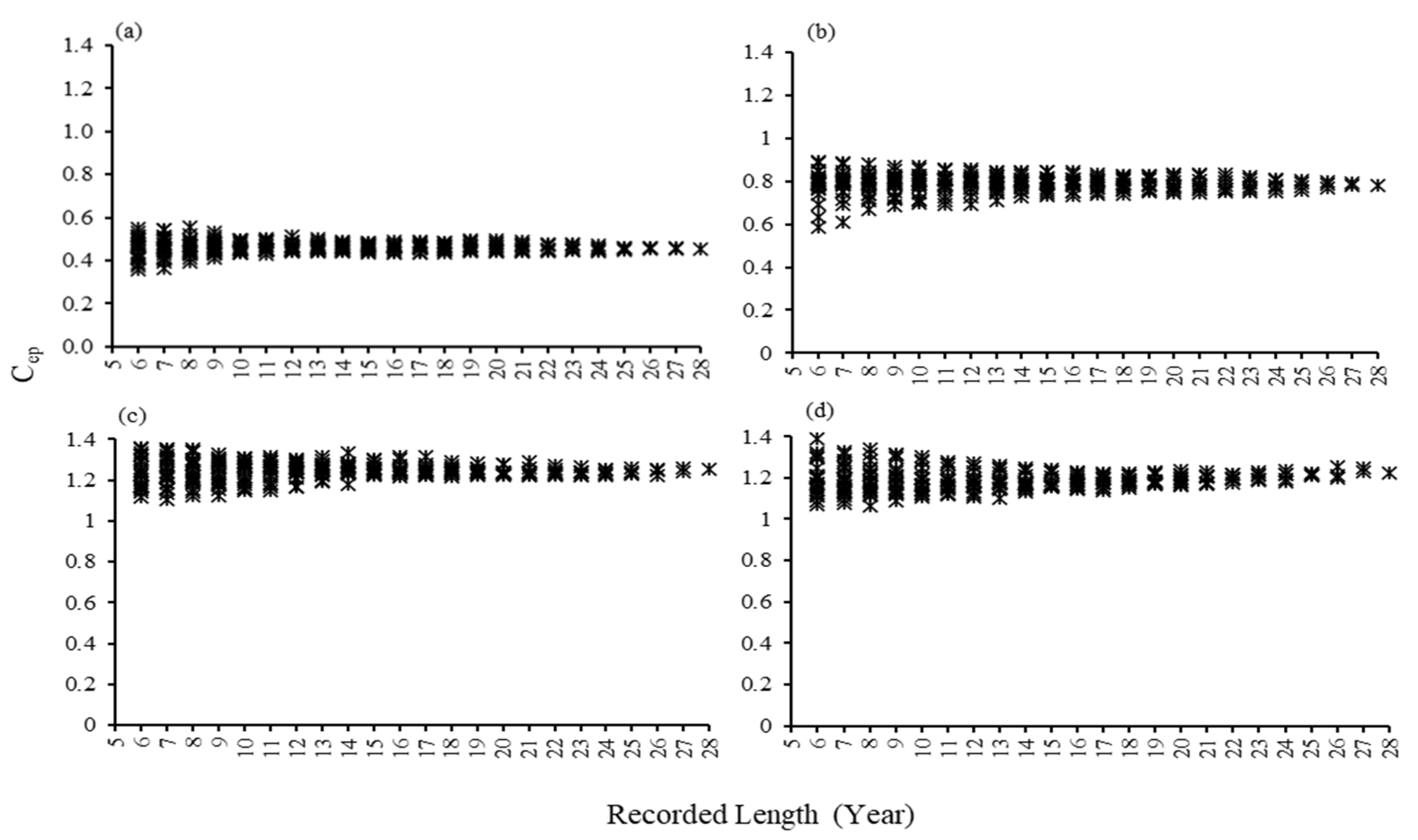
Before the model simulation was accomplished, the results of Cep values for four different river basins, which have been sensitive on the annual scale using the aridity index, were described in Figure 1. Accordingly, the Cep values calculated from the longer data length showed less variation than the shorter data length.
3.1.1. Annual Nash Results for the 28-Year Dataset
Using the estimated Cep values mentioned in Section 3.1, corresponding with the optimized parameters for four river basins; (Doki River Basin, the Nantahala River basin, MOPEX ID: 03504000; the Oostanaula River basin, MOPEX ID: 02387500; and the Noxubee River basin, ID: 02448000), the Nash values in daily, monthly, and annual scale were executed by running the XAJ model with 28-year datasets as in Figure 2. In addition, annual Nash values considering 28-year datasets were considered as it helps determine the minimum data length with the comparison of annual Nash values of subsets, as shown in Figure 2.
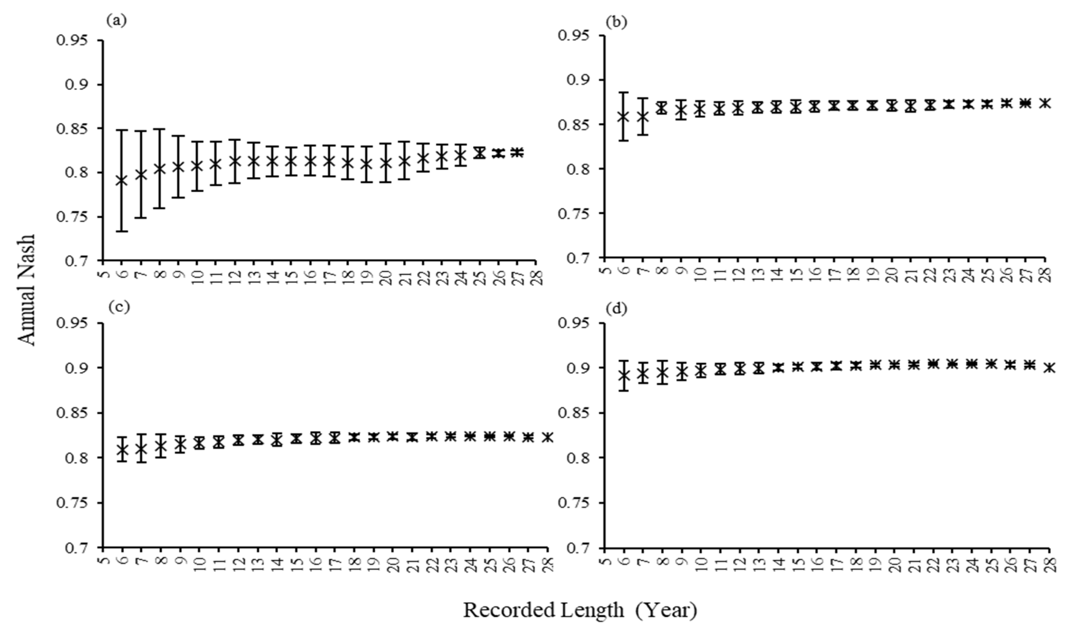
The values of the average and standard deviation Nash efficiency values were plotted to better understand the behaviors of the results, as in Figure 3. According to Figure 3, the standard deviation values by calibrating the model using a 28-dataset in four river basins did not show much fluctuation in the model results. These results suggested that using longer datasets in model calibration in all four river basins has good results.
3.1.2. Annual Nash Results for Subsets
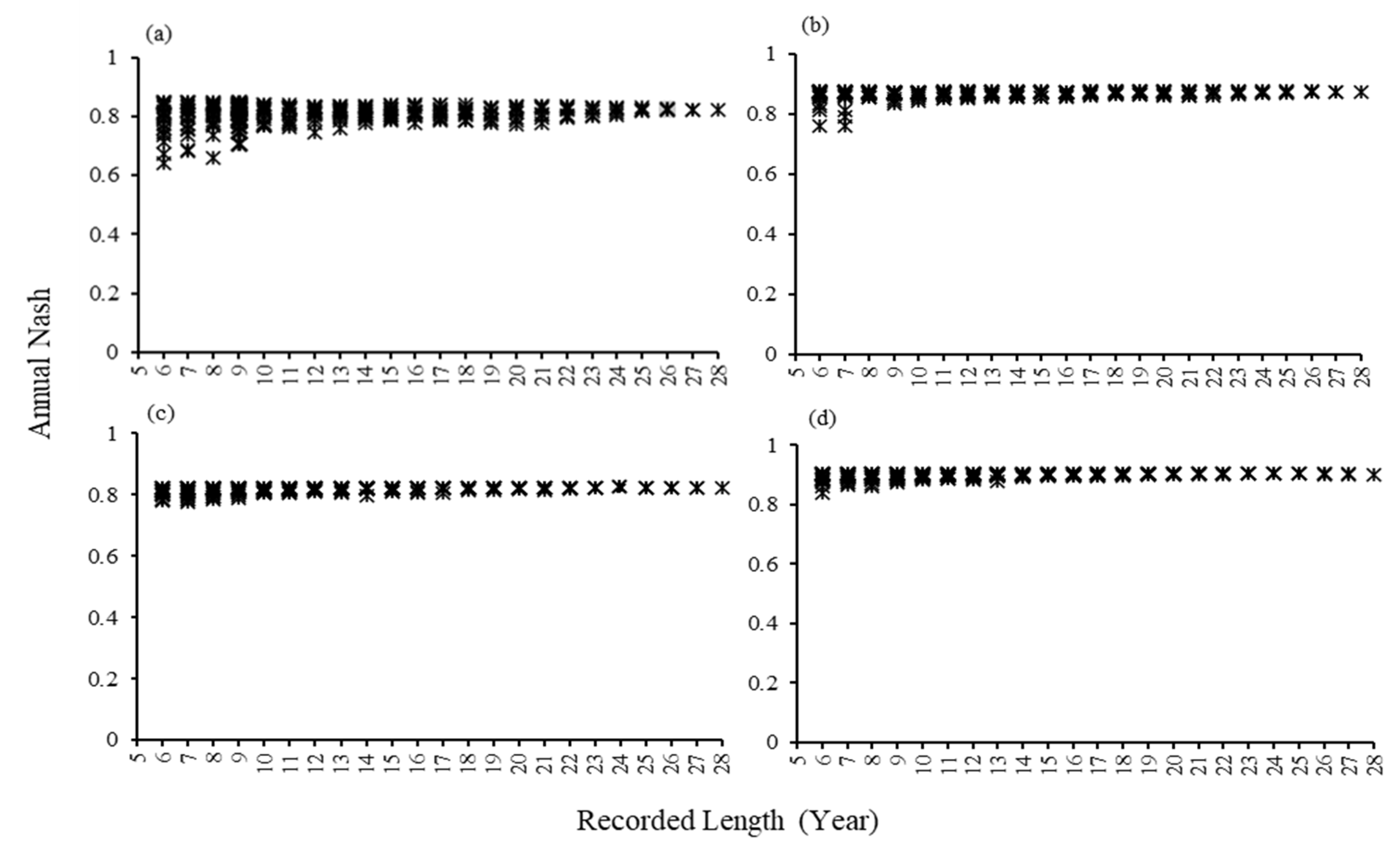
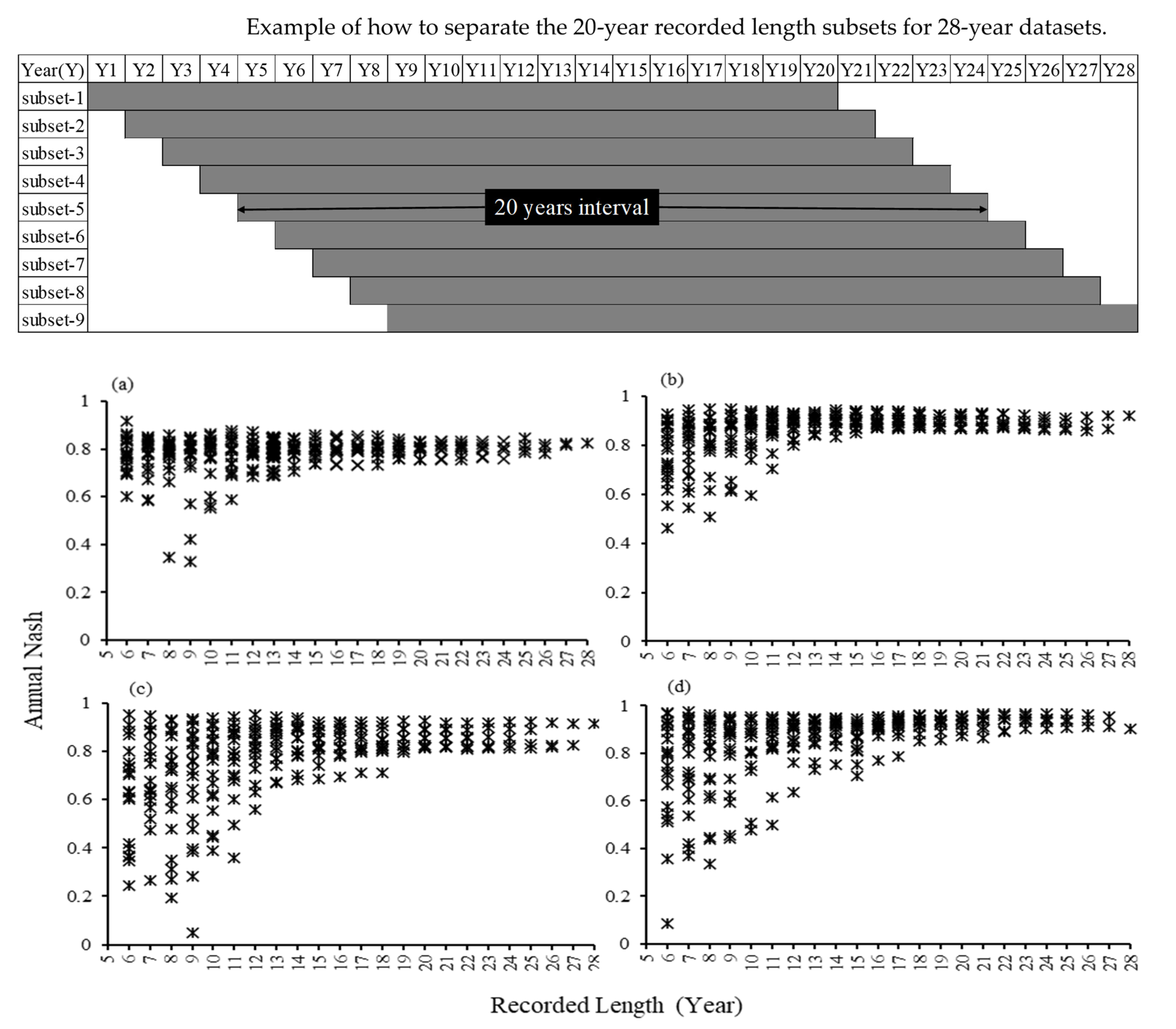
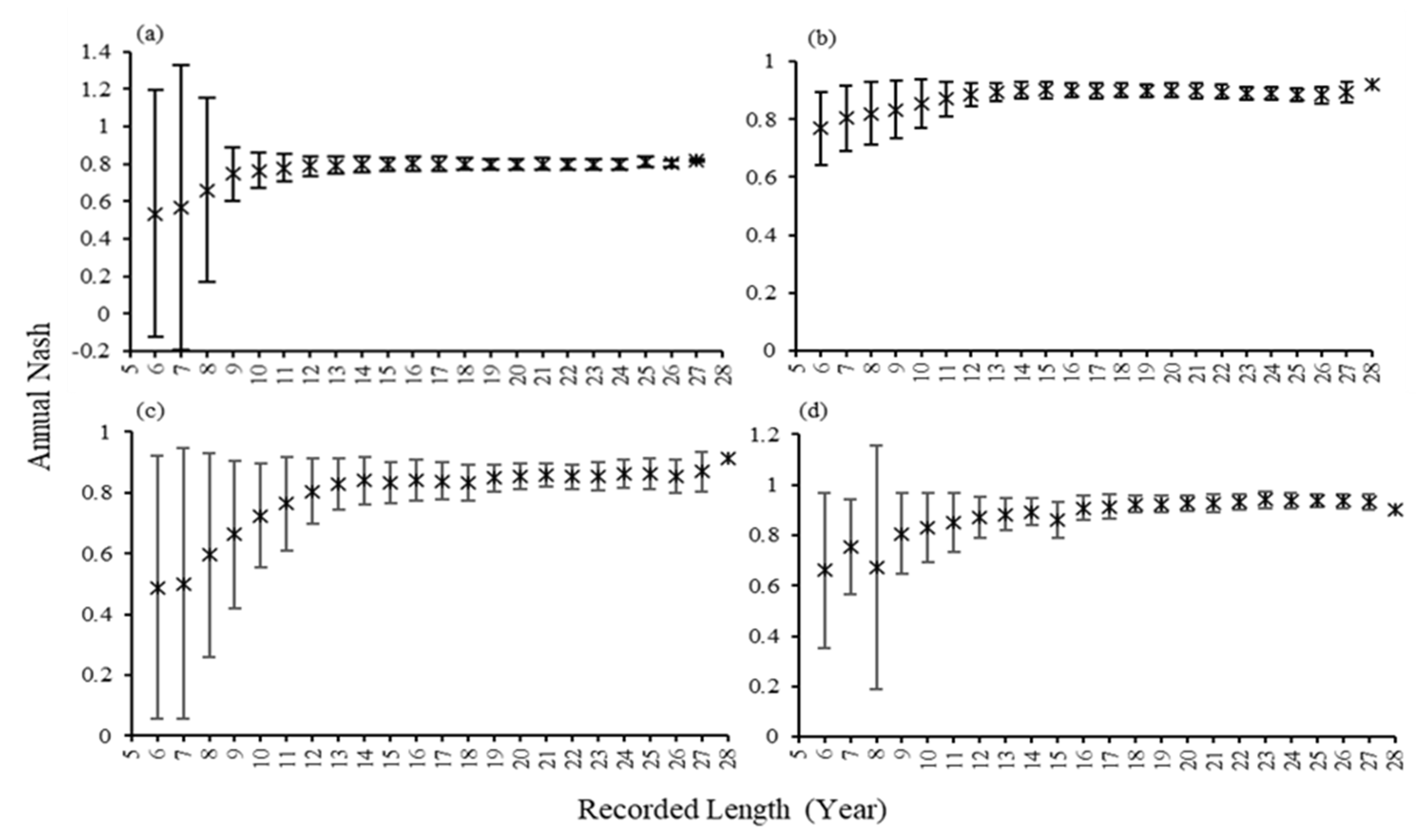
As mentioned in the previous section, the 28-year datasets from each of the four river basins were divided into different subsets with consecutive years in Table 4. The model’s performance was evaluated by calibrating the model using those different subsets from 6-year to 28-year data length, and the annual Nash values are shown in Figure 4. There was a steep variation between 6-year and 9-year subsets in all four river basins after calculating the average and standard deviation values over the model results. Apart from the model calibration with 28-year datasets, the difference in standard deviation values occurred while calibrating the model with a shorter data length.
However, with the data length of the subsets increasing from 10-year, the variation of standard deviation values became less fluctuated without a dramatic difference, according to Figure 5.
3.1.3. Comparative Evaluation of Nash Results between 28-Year Datasets and Subsets
This section compares the model calibration results between 28-year datasets and subsets to provide robust information in considering the minimum length of datasets depending on the efficiency measures utilized to evaluate the simulation performance. The model’s performance increases as Nash efficiency values increase [59]. Additionally, it will be feasible to presume the behavior of the Nash efficiency results across the minimum acceptable data length.
Relying on Nash results, the performance of the model can be assessed. Therefore, it is possible to explicitly demonstrate how the Nash efficiency varies with dataset length by comparing the Nash values of the model calibrated with 28-year datasets and subsets.
The calibration with 28-year datasets shows good annual Nash values. However, while calibrating the model with subsets, the results in shorter data lengths are unstable and show data fluctuation between 6-year and 10-year datasets. However, starting from 10-year datasets, the model results show a similar pattern running with the 28-year dataset. Therefore, in this research, estimating the parameter values and calibrating annual Nash efficiency values over the shorter datasets shows less information than the longer ones. This way can be possible to show how the Nash varies according to how long the length of the datasets is. According to this comparison between 28-year datasets and sub-sets, starting from 10-year datasets, the standard deviation values are consistent and show no significant variations in all river basins. Hence, it can be assumed that starting from 10-year subsets is best suited to run the XAJ model to obtain adequate information to improve the performance of the XAJ model. However, this study continued to prove these findings using theoretical-based analysis in Section 3.1.4.
3.1.4. Hypothesis Analysis over Subsets
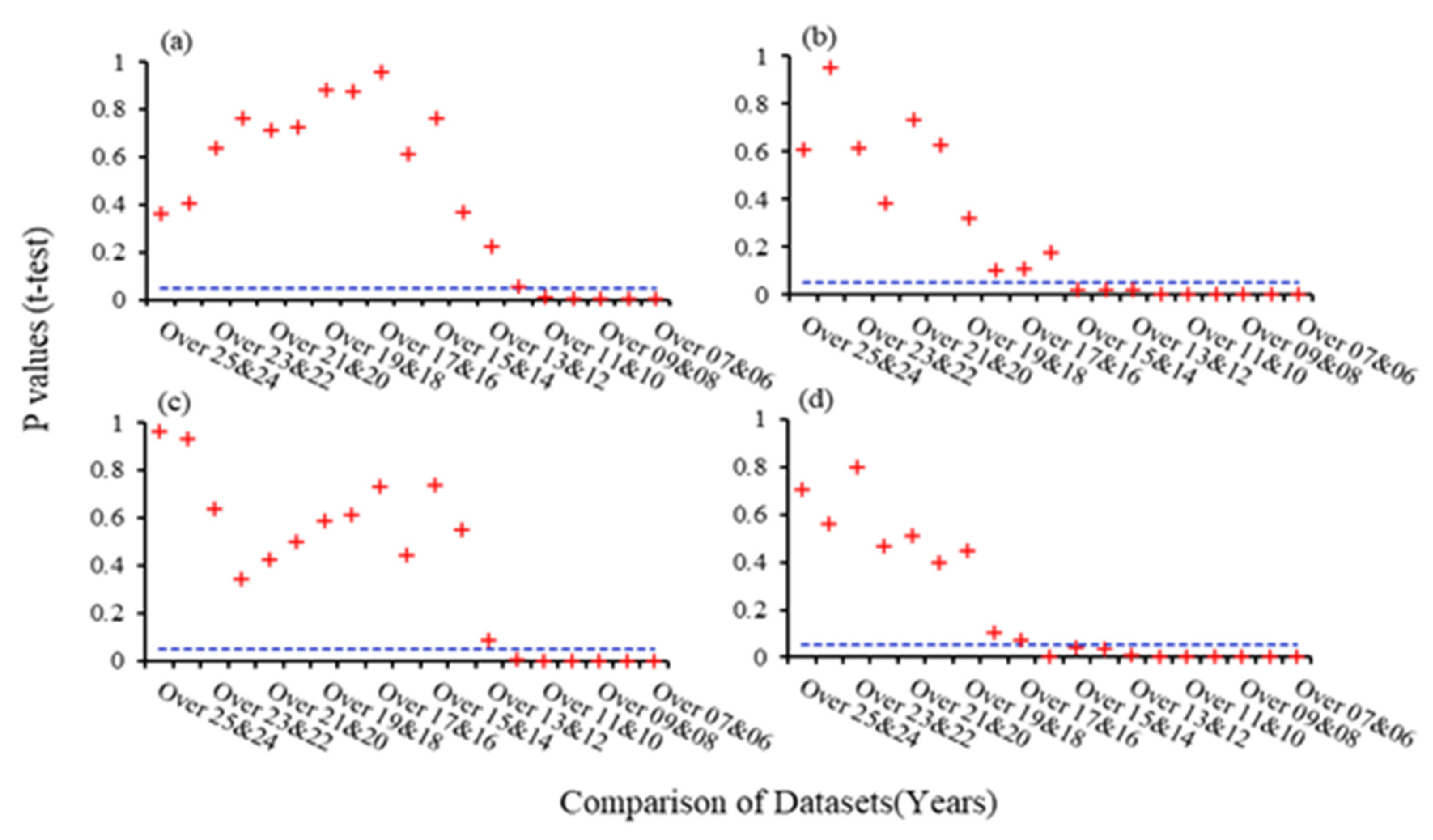
This section aims to help to estimate the most acceptable minimum data lengths in all study basins. The central part of this analysis consists of testing 19 different datasets comparisons with varying lengths and observation periods in each study river basin. Two subsets of different data lengths were selected and statistically analyzed each time to hypothetically prove the significant difference between the Nash results. Two samples unpaired t-test was applied using a 5% confidence interval using the statistical software (JMP 16). The two-sided test results were selected and compared to decide the acceptable minimum data length theoretically. According to the test results with a significant level shown in Figure 6, it can be hypothetically proved that starting from 10-year data length for Doki River Basin, 11-year data length for ID 03504000, 12-year data length for ID 02387500, and 13-year data length for ID 02448000 were hypothetically significant during the tests. Hence, it can be proven as the most acceptable minimum data length.
3.2. Analysis of the Impacts of Datasets Using Regression Analysis
The regression analysis based on the coefficient of evapotranspiration Cep was performed according to the results of the previous session about how the errors in observed datasets can affect the impacts on the parameter estimation and model performance. The instrumental error may bias the interpretation of Nash efficiency values in observed datasets, the length and number of data, outliers, and repeated data. Hence, detecting outliers in observed datasets usually plays an essential role in data monitoring. The observation departs from other observations to create doubt that a different mechanism caused it can be called an outlier [60], or data designs deviate from a well-defined concept of typical behavior [61]. The amount of change in a parameter associated with Nash efficiency values can be summarized using regression analysis to examine statistical significance with Equation (6). This method developed by [44] proved the easy and effective calculation of complex parameter estimation. However, it will rely on the size of the datasets and whether the annual runoff coefficient, as well as the pan aridity index, are correlated. Regression equations can help find the many predictive or relation equations in the literature and hydrological parameters. Regression analysis is often used as a simple x-y graph.
However, in practical conditions with distributions of actual data, it is not easy to find that all the data points fit precisely through them. Therefore, the two-variable regression model defines one variable as independent and the other as a dependent variable. According to [44], Cep was calculated in this study using the logarithmic form of Equation (6). According to Equation (6), the annual runoff coefficient was used as the dependent variable and the pan aridity index as the independent variable. Here, the coefficients, m and n, can be calculated using curve fitting.
The purpose of outlier detection in this study is to compare the performance of Cep before and after removing outliers compared with the simulated Cep value.
3.2.1. Calculation of Simulated (Optimized Cep) in Four River Basins
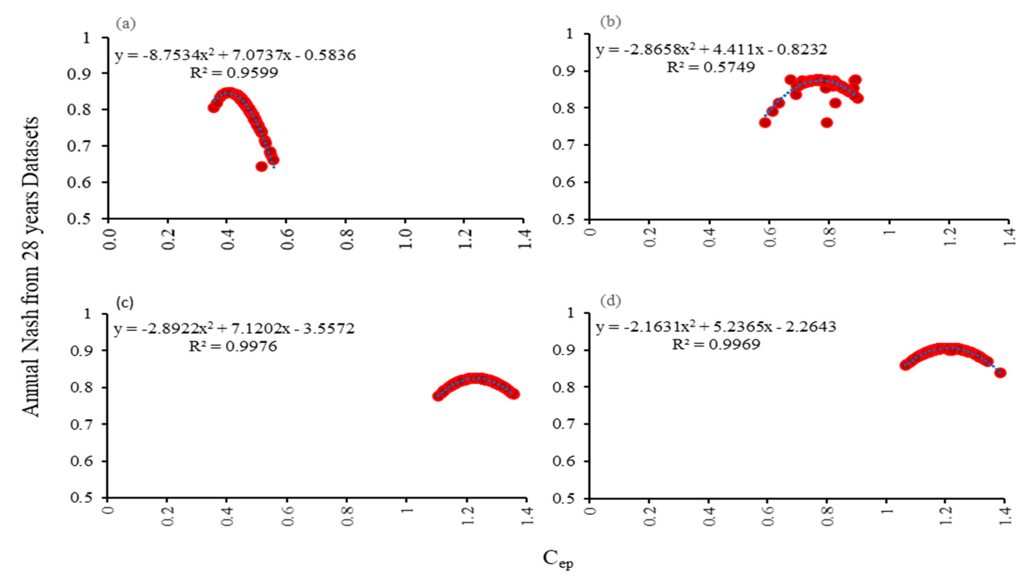
The simulated Cep values in four river basins were initially calculated based on the annual Nash values of 28-year datasets by the polynomial regression analysis using Equation (6), as shown in Figure 7. The purpose of calculating the simulated Cep was to compare the simulated values with the changes in parameter Cep values before and after removing outliers in both the 28-year dataset and subsets in all basins. The values of simulated values are shown in Figure 7.
3.2.2. Regression Analysis in the 28-year Dataset
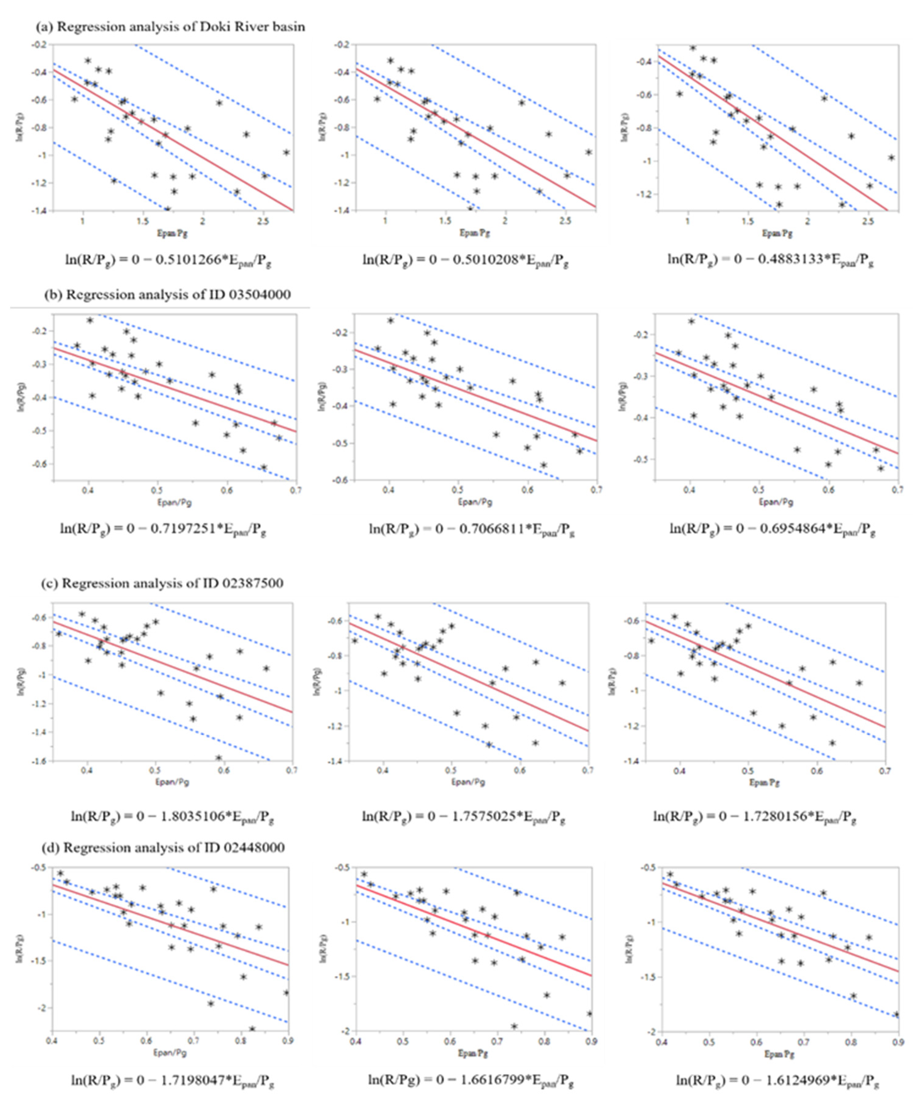
Figure 8 shows the regression analysis results performed in each basin with 95 percent confidence intervals. According to Figure 8, the small interval is the confidence interval, and the large interval is the prediction interval. Firstly, the regression analysis over the 28-year dataset for four river basins, Doki River Basin (from 1978 to 2005); ID 3504000 (from 1974 to 2001), ID 2387500 (from 1974 to 2001), and ID 2448000 (from 1962 to 1989) was performed to find the outliers in each 28-year datasets. As the data length of 28-year was sufficient to perform the regression analysis three times, the Cep values before and after removing outliers can be discussed clearly in this section. According to the first regression analysis, the outlier year in each basin (for Doki River Basin, ID 3504000, ID 2387500, and ID 2448000) was 1987, 2000, 1988, and 1963, as those years were observed outside of the prediction interval as shown in Figure 8. Removing these outlier years from each dataset improved the parameter optimization, and the second regression analysis was calculated again with the 27-year datasets. After removing outliers, the Cep values became closer to the simulated Cep (the Cep calculated from using the best performance Nash values with 28-year datasets). Therefore, it can be said that removing outliers can contribute to the remarkable effectiveness of parameter estimation. In this case, regression analysis was performed for the third time to highlight its effectiveness in removing outliers among the datasets. Similar to the previous calculations, it can be proved that removing the unstable years as outliers from observed datasets can attain the Cep values closer to the simulated Cep values and improve the performance of parameter estimation, as shown in Table 5. Therefore, removing outliers can contribute to better parameter optimization, which can impact model performance apart from data scarcity.
3.2.3. Regression Analysis in Subsets
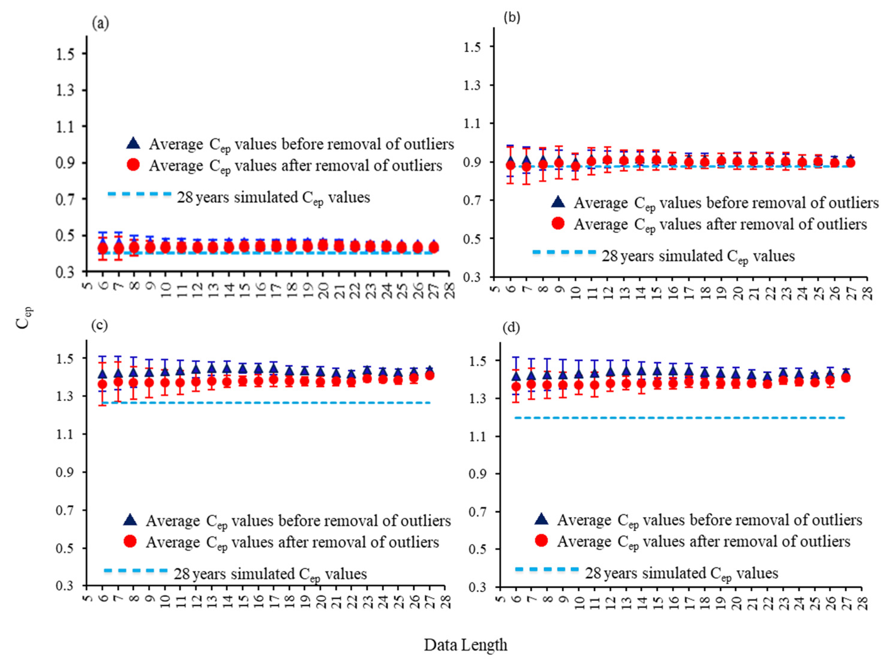
For shorter datasets, performing the repeated regression analysis to remove the outliers is difficult due to data scarcity. Therefore, the outlier removal using regression analysis was performed only once for each different data length of subsets (from 6-year to 27-year data length subsets) in all four study basins. Figure 9 shows average and standard deviation values of Cep for all different subsets from each river basin before and after removing outliers.
According to the comparison results with the simulated Cep, after removing outliers in each subset, Cep was becoming more similar to the simulated values in all study basins, as shown in Figure 9. Therefore, as a result, it can be assumed that the removal of outliers by applying regression analysis across the subsets can also be effective for parameter estimation and model calibration.
4. Conclusions
Firstly, this research analyses the most acceptable minimum data length using the 28-year datasets from four river basins of different locations and characteristics using the XAJ model. In this case, the aridity index method is applied for parameter optimization to narrow the parameter space between the most sensitive parameters, Cp and Cep. For the estimation of the model performance, the annual Nash efficiency approach is used to compare the results between the 28-year dataset and subsets using a statistical approach. Therefore, the application of hypothesis analysis over the annual Nash results of the XAJ model in four different river basins from Japan and U.S. basins is applied to help prove the acceptable minimum data length between 6-year to 28-year datasets statistically significant. It is possible to observe that using longer datasets can improve the model performance.
According to the hypothesis analysis, the test results for Doki River Basin, ID 3504000, ID 2387500, and ID 2448000 are 10-, 11-,12-, and 13-year, respectively, hypothetically significant at a 5% confidence level. Therefore, it can be proved that datasets between 10- and 13-year data length can be used as the acceptable minimum data length in the studied catchments for model calibration and flood forecasting in data-scarce basins.
Based on the previous results, it can be observed clearly that there are some abnormal behaviors in the annual Nash results of shorter subsets. Therefore, based on the error or abnormal behaviors of the observed datasets, this study tried to prove that these behaviors can affect parameter estimation, leading to the model’s performance using regression analysis. According to regression analysis, removing outliers from the original datasets can improve the parameter estimation in both the 28-year dataset and subsets in all study basins. Therefore, removing outliers in datasets can improve parameter calculation, affecting the model performance and the selection of the minimum data length.
This study has some limitations with the basin characteristics and geology of the study basins. Apart from the limitations (groundwater, vegetation cover, and aridity index in deciding the acceptable minimum data length) and the assumptions (the coefficient of evaporation value, the selection of basins without considering the snow, and the consideration of the statistical significance in the hypothesis analysis), this study will be helpful to decide the most acceptable minimum data length in the data-scarce regions, especially in developing countries which plays the controversial role among hydrologists.
We intend to explore the relationship between the minimum data length and aridity index (soil moisture memory) as a further study for estimating data length, which can impact the estimation of minimum data length.
Author Contributions
Conceptualization, T.T.Z. and M.L.; methodology, T.T.Z. and M.L.; software, T.T.Z.; validation, T.T.Z.; formal analysis, T.T.Z.; investigation, T.T.Z. and M.L.; resources, M.L.; data curation, T.T.Z. and M.L.; writing—original draft preparation, T.T.Z.; writing—review and editing, T.T.Z. and M.L.; visualization, T.T.Z.; supervision, M.L.; project administration, M.L. All authors have read and agreed to the published version of the manuscript.
Funding
This research received no external funding.
Institutional Review Board Statement
Not applicable.
Informed Consent Statement
Not applicable.
Data Availability Statement
Information on all the data applied in this research is shown in Section 2 in detail.
Conflicts of Interest
Regarding this paper and the research, the authors state that they have no conflicts of interest.
References
- Perry, L.K. Water Resources Research Institute. Wyo. Univ. Water Resour. Res. Inst. Water Resour. Ser. 1974, 44, 4823–4839. [Google Scholar]
- Lidén, R.; Harlin, J. Analysis of conceptual rainfall–runoff modelling performance in different climates. J. Hydrol. 2000, 238, 231–247. [Google Scholar] [CrossRef]
- Jain, S.K.; Mani, P.; Jain, S.K.; Prakash, P.; Singh, V.P.; Tullos, D.; Kumar, S.; Agarwal, S.P.; Dimri, A.P. A Brief review of flood forecasting techniques and their applications. Int. J. River Basin Manag. 2018, 16, 329–344. [Google Scholar] [CrossRef]
- Ronco, P.; Gallina, V.; Torresan, S.; Zabeo, A.; Semenzin, E.; Critto, A.; Marcomini, A. The KULTURisk Regional Risk Assessment methodology for water-related natural hazards—Part 1: Physical–environmental assessment. Hydrol. Earth Syst. Sci. 2014, 18, 5399–5414. [Google Scholar] [CrossRef]
- Tingsanchali, T. Urban flood disaster management. Procedia Eng. 2012, 32, 25–37. [Google Scholar] [CrossRef]
- Cvetkovic, V.M.; Martinović, J. Innovative Solutions for Flood Risk Management. Int. J. Disaster Risk Manag. 2020, 2, 71–99. [Google Scholar] [CrossRef]
- Ming, X.; Liang, Q.; Xia, X.; Li, D.; Fowler, H.J. Real-Time Flood Forecasting Based on a High-Performance 2-D Hydrodynamic Model and Numerical Weather Predictions. Water Resour. Res. 2020, 56, e2019WR025583. [Google Scholar] [CrossRef]
- Dibike, Y.; Solomatine, D. River flow forecasting using artificial neural networks. Phys. Chem. Earth Part B Hydrol. Ocean. Atmos. 2001, 26, 1–7. [Google Scholar] [CrossRef]
- Todini, E. Hydrological catchment modelling: Past, present and future. Hydrol. Earth Syst. Sci. 2007, 11, 468–482. [Google Scholar] [CrossRef]
- Nayak, P.; Venkatesh, B.; Krishna, B.; Jain, S.K. Rainfall-runoff modeling using conceptual, data driven, and wavelet based computing approach. J. Hydrol. 2013, 493, 57–67. [Google Scholar] [CrossRef]
- Chen, H.; Xu, C.-Y.; Guo, S. Comparison and evaluation of multiple GCMs, statistical downscaling and hydrological models in the study of climate change impacts on runoff. J. Hydrol. 2012, 434–435, 36–45. [Google Scholar] [CrossRef]
- Hapuarachchi, H.A.P.; Li, Z.; Wang, S. Application of SCE-UA Method for Calibrating the Xinanjiang Watershed Model. J. Lake Sci. 2001, 13, 304–314. [Google Scholar] [CrossRef]
- Perrin, C.; Oudin, L.; Andréassian, V.; Serna, C.R.; Michel, C.; Mathevet, T. Impact of limited streamflow data on the efficiency and the parameters of rainfall—Runoff models. Hydrol. Sci. J. 2007, 52, 131–151. [Google Scholar] [CrossRef]
- Li, X.; Lu, M. Multi-step Optimization of Parameters in the Xinanjiang Model Taking into Account Their Time Scale Dependency. J. Jpn. Soc. Civ. Eng. Ser. B1 (Hydraul. Eng.) 2012, 68, I_145–I_150. [Google Scholar] [CrossRef]
- Bloschl, G.; Reszler, C.; Komma, J. A spatially distributed flash flood forecasting model. Environ. Model. Softw. 2008, 23, 464–478. [Google Scholar] [CrossRef]
- Niemczynowicz, J. Urban hydrology and water management—Present and future challenges. Urban Water 1999, 1, 1–14. [Google Scholar] [CrossRef]
- Krajewski, W.; Smith, J. Radar hydrology: Rainfall estimation. Adv. Water Resour. 2002, 25, 1387–1394. [Google Scholar] [CrossRef]
- Yan, K.; Di Baldassarre, G.; Solomatine, D.P.; Schumann, G.J. A review of low-cost space-borne data for flood modelling: Topography, flood extent and water level. Hydrol. Process. 2015, 29, 3368–3387. [Google Scholar] [CrossRef]
- Al-Sabhan, W.; Mulligan, M.; Blackburn, G. A real-time hydrological model for flood prediction using GIS and the WWW. Comput. Environ. Urban Syst. 2003, 27, 9–32. [Google Scholar] [CrossRef]
- Brath, A.; Montanari, A.; Toth, E. Analysis of the effects of different scenarios of historical data availability on the calibration of a spatially-distributed hydrological model. J. Hydrol. 2004, 291, 232–253. [Google Scholar] [CrossRef]
- Pappenberger, F.; Thielen, J.; Del Medico, M. The impact of weather forecast improvements on large scale hydrology: Analysing a decade of forecasts of the European Flood Alert System. Hydrol. Process. 2011, 25, 1091–1113. [Google Scholar] [CrossRef]
- Sorooshian, S.; Gupta, V.K.; Fulton, J.L. Evaluation of Maximum Likelihood Parameter estimation techniques for conceptual rainfall-runoff models: Influence of calibration data variability and length on model credibility. Water Resour. Res. 1983, 19, 251–259. [Google Scholar] [CrossRef]
- Li, C.Z.; Wang, H.; Liu, J.; Yan, D.H.; Yu, F.L.; Zhang, L. Effect of calibration data series length on performance and optimal parameters of hydrological model. Water Sci. Eng. 2010, 3, 378–393. [Google Scholar] [CrossRef]
- Finger, D.; Vis, M.; Huss, M.; Seibert, J. The value of multiple data set calibration versus model complexity for improving the performance of hydrological models in mountain catchments. Water Resour. Res. 2015, 51, 1939–1958. [Google Scholar] [CrossRef]
- Weiss, M.; Jacob, F.; Duveiller, G. Remote sensing for agricultural applications: A meta-review. Remote Sens. Environ. 2019, 236, 111402. [Google Scholar] [CrossRef]
- Hughes, D.; Kapangaziwiri, E.; Sawunyama, T. Hydrological model uncertainty assessment in southern Africa. J. Hydrol. 2010, 387, 221–232. [Google Scholar] [CrossRef]
- Chen, L.; Xu, J.; Wang, G.; Shen, Z. Comparison of the multiple imputation approaches for imputing rainfall data series and their applications to watershed models. J. Hydrol. 2019, 572, 449–460. [Google Scholar] [CrossRef]
- Güntner, A. Improvement of Global Hydrological Models Using GRACE Data. Surv. Geophys. 2008, 29, 375–397. [Google Scholar] [CrossRef]
- Hattermann, F.F.; Krysanova, V.; Gosling, S.N.; Dankers, R.; Daggupati, P.; Donnelly, C.; Flörke, M.; Huang, S.; Motovilov, Y.; Buda, S.; et al. Cross-scale intercomparison of climate change impacts simulated by regional and global hydrological models in eleven large river basins. Clim. Chang. 2017, 141, 561–576. [Google Scholar] [CrossRef]
- Winsemius, H.C.; Schaefli, B.; Montanari, A.; Savenije, H.H.G. On the calibration of hydrological models in ungauged basins: A framework for integrating hard and soft hydrological information. Water Resour. Res. 2009, 45, e2009wr007706. [Google Scholar] [CrossRef]
- Pellicciotti, F.; Buergi, C.; Immerzeel, W.W.; Konz, M.; Shrestha, A.B. Challenges and Uncertainties in Hydrological Modeling of Remote Hindu Kush–Karakoram–Himalayan (HKH) Basins: Suggestions for Calibration Strategies. Mt. Res. Dev. 2012, 32, 39–50. [Google Scholar] [CrossRef]
- Harlin, J. Development of a Process Oriented Calibration Scheme for the HBV Hydrological Model. Hydrol. Res. 1991, 22, 15–36. [Google Scholar] [CrossRef]
- Yapo, P.O.; Gupta, H.V.; Sorooshian, S. Automatic calibration of conceptual rainfall-runoff models: Sensitivity to calibration data. J. Hydrol. 1996, 181, 23–48. [Google Scholar] [CrossRef]
- Gan, T.Y.; Biftu, G.F. Automatic Calibration of Conceptual Rainfall-Runoff Models: Optimization Algorithms, Catchment Conditions, and Model Structure. Water Resour. Res. 1996, 32, 3513–3524. [Google Scholar] [CrossRef]
- Huang, Q.; Qin, G.; Zhang, Y.; Tang, Q.; Liu, C.; Xia, J.; Chiew, F.H.S.; Post, D. Using Remote Sensing Data-Based Hydrological Model Calibrations for Predicting Runoff in Ungauged or Poorly Gauged Catchments. Water Resour. Res. 2020, 56, e2020WR028205. [Google Scholar] [CrossRef]
- Anctil, F.; Perrin, C.; Andréassian, V. Impact of the length of observed records on the performance of ANN and of conceptual parsimonious rainfall-runoff forecasting models. Environ. Model. Softw. 2004, 19, 357–368. [Google Scholar] [CrossRef]
- Boughton, W. Large sample basin experiments for hydrological model parameterization: Results of the model parameter experiment—MOPEX. Aust. J. Water Resour. 2007, 11, 119–120. [Google Scholar]
- Beven, K. Rainfall-Runoff Modelling: The Primer; John Wiley & Sons: New York, NY, USA, 2011. [Google Scholar]
- Lu, M. Recent and future studies of the Xinanjiang Model. J. Hydraul. Eng. 2021, 52, 432–441. [Google Scholar] [CrossRef]
- Azida, A.; Bakar, A.B.U.; Lu, M. Effects of temporal resolution on river flow forecasting with simple interception model within a distributed hydrological model. Int. J. Res. Rev. Appl. Sci. 2011, 8, 5–13. [Google Scholar]
- Duan, Q.; Schaake, J.; Andréassian, V.; Franks, S.; Goteti, G.; Gupta, H.; Gusev, Y.; Habets, F.; Hall, A.; Hay, L.; et al. Model Parameter Estimation Experiment (MOPEX): An overview of science strategy and major results from the second and third workshops. J. Hydrol. 2006, 320, 3–17. [Google Scholar] [CrossRef]
- Arora, V.K. The use of the aridity index to assess climate change effect on annual runoff. J. Hydrol. 2002, 265, 164–177. [Google Scholar] [CrossRef]
- Quan, C.; Han, S.; Utescher, T.; Zhang, C.; Liu, Y.-S. Validation of temperature–precipitation based aridity index: Paleoclimatic implications. Palaeogeogr. Palaeoclim. Palaeoecol. 2013, 386, 86–95. [Google Scholar] [CrossRef]
- Li, X.; Lu, M. Application of Aridity Index in Estimation of Data Adjustment Parameters in the Xinanjiang Model, Jstage.Jst.Go.Jp. 58. 2014. Available online: https://www.jstage.jst.go.jp/article/jscejhe/70/4/70_28/_article/-char/ja/ (accessed on 25 June 2022).
- Schreiber, P. About the relationship between precipitation and the flow of water in rivers in Central Europe. Z. Meteorol. 1904, 21, 441–452. (In German) [Google Scholar]
- Budyko, M.I. Evaporation under Natural Conditions, Gidrometeorizdat, Leningrad; IPST: Jerusalem, Israel, 1948; Volume 635. [Google Scholar]
- Zhao, R.-J. The Xinanjiang model applied in China. J. Hydrol. 1992, 135, 371–381. [Google Scholar]
- Kyi, K.H.; Lu, M.; Li, X. Development of a user-friendly web-based rainfall-runoff model. Hydrol. Res. Lett. 2016, 10, 8–14. [Google Scholar] [CrossRef] [Green Version]
- Zhao, R.J.; Liu, X.R. The Xinanjiang Model. In Computer Models of Watershed Hydrology; Singh, V.P., Ed.; Water Resources Publications: Highlands Ranch, CO, USA, 1995; pp. 215–232. [Google Scholar]
- Rahman, M.M.; Lu, M.; Kyi, K.H. Variability of soil moisture memory for wet and dry basins. J. Hydrol. 2015, 523, 107–118. [Google Scholar] [CrossRef]
- Knoben, W.J.M.; Freer, J.E.; Woods, R.A. Technical note: Inherent benchmark or not? Comparing Nash–Sutcliffe and Kling–Gupta efficiency scores. Hydrol. Earth Syst. Sci. 2019, 23, 4323–4331. [Google Scholar] [CrossRef]
- Beven, K.; Freer, J. Equifinality, data assimilation, and uncertainty estimation in mechanistic modelling of complex environmental systems using the GLUE methodology. J. Hydrol. 2001, 249, 11–29. [Google Scholar] [CrossRef]
- Schaefli, B.; Gupta, H.V. Do Nash values have value? Hydrol. Process. 2007, 21, 2075–2080. [Google Scholar] [CrossRef]
- Nash, J.E.; Sutcliffe, J.V. River flow forecasting through conceptual models part I—A discussion of principles. J. Hydrol. 1970, 10, 282–290. [Google Scholar] [CrossRef]
- Pfister, L.; Kirchner, J.W. Debates-Hypothesis testing in hydrology: Theory and practice. Water Resour. Res. 2017, 53, 1792–1798. [Google Scholar] [CrossRef]
- Naghettini, M. (Ed.) Fundamentals of Statistical Hydrology; Springer: Berlin, Germany, 2017. [Google Scholar] [CrossRef]
- Stevens, J.P. Outliers and influential data points in regression analysis. Psychol. Bull. 1984, 95, 334–344. [Google Scholar] [CrossRef]
- Refsgaard, J.C.; Knudsen, J. Operational Validation and Intercomparison of Different Types of Hydrological Models. Water Resour. Res. 1996, 32, 2189–2202. [Google Scholar] [CrossRef]
- Lu, M.; Li, X. Time scale dependent sensitivities of the XinAnJiang model parameters. Hydrol. Res. Lett. 2014, 8, 51–56. [Google Scholar] [CrossRef] [Green Version]
- Colla, V.; Vannucci, M. Outlier Detection Methods for Industrial Applications. In Advances in Robotics, Automation and Control; BoD-Books on Demand: Norderstedt, Germany, 2008. [Google Scholar] [CrossRef] [Green Version]
- Chandola, V.; Banerjee, A.K.-V. Computing Surveys (CSUR), Undefined 2009, Anomaly Detection: A Survey, Dl.Acm.Org. 2009. Available online: https://dl.acm.org/doi/abs/10.1145/1541880.1541882 (accessed on 25 June 2022).
Figure 1.
The values of Cep for (a) Doki River Basin (b) MOPEX ID 3504000 (c) MOPEX ID 2387500 and (d) MOPEX ID 2448000.
Figure 1.
The values of Cep for (a) Doki River Basin (b) MOPEX ID 3504000 (c) MOPEX ID 2387500 and (d) MOPEX ID 2448000.

Figure 2.
The values of annual Nash in all 28-year datasets for (a) Doki River Basin (b) MOPEX ID 3504000 (c) MOPEX ID 2387500 and (d) MOPEX ID 2448000.
Figure 2.
The values of annual Nash in all 28-year datasets for (a) Doki River Basin (b) MOPEX ID 3504000 (c) MOPEX ID 2387500 and (d) MOPEX ID 2448000.

Figure 3.
The values of average and standard deviation of annual Nash in all 28-year datasets for (a) Doki River Basin, (b) MOPEX ID 3504000, (c) MOPEX ID 2387500, and (d) MOPEX ID 2448000.
Figure 3.
The values of average and standard deviation of annual Nash in all 28-year datasets for (a) Doki River Basin, (b) MOPEX ID 3504000, (c) MOPEX ID 2387500, and (d) MOPEX ID 2448000.

Figure 4.
The values of annual Nash in subsets for (a) Doki River Basin (b) MOPEX ID 3504000 (c) MOPEX ID 2387500 and (d) MOPEX ID 2448000.
Figure 4.
The values of annual Nash in subsets for (a) Doki River Basin (b) MOPEX ID 3504000 (c) MOPEX ID 2387500 and (d) MOPEX ID 2448000.

Figure 5.
The values of average and standard deviation of annual Nash in subsets for (a) Doki River Basin, (b) MOPEX ID 3504000, (c) MOPEX ID 2387500, and (d) MOPEX ID 2448000.
Figure 5.
The values of average and standard deviation of annual Nash in subsets for (a) Doki River Basin, (b) MOPEX ID 3504000, (c) MOPEX ID 2387500, and (d) MOPEX ID 2448000.

Figure 6.
Hypothesis test results for (a) Doki River Basin (b) MOPEX ID 3504000 (c) MOPEX ID 2387500 and (d) MOPEX ID 2448000. + + + p values resulting from the comparison of subsets; ------ Values of 5% Confidence Interval.
Figure 6.
Hypothesis test results for (a) Doki River Basin (b) MOPEX ID 3504000 (c) MOPEX ID 2387500 and (d) MOPEX ID 2448000. + + + p values resulting from the comparison of subsets; ------ Values of 5% Confidence Interval.

Figure 7.
Polynomial regression analysis for simulated Cep values in (a) Doki River Basin (b) MOPEX ID 3504000 (c) MOPEX ID 2387500 and (d) MOPEX ID 2448000.
Figure 7.
Polynomial regression analysis for simulated Cep values in (a) Doki River Basin (b) MOPEX ID 3504000 (c) MOPEX ID 2387500 and (d) MOPEX ID 2448000.

Figure 8.
Stages of regression analysis in 28-year datasets for Cep values before and after removing outliers in (a) Doki River Basin, (b) MOPEX ID 3504000, (c) MOPEX ID 2387500, and (d) MOPEX ID 2448000.
Figure 8.
Stages of regression analysis in 28-year datasets for Cep values before and after removing outliers in (a) Doki River Basin, (b) MOPEX ID 3504000, (c) MOPEX ID 2387500, and (d) MOPEX ID 2448000.

Figure 9.
Comparison of Cep values in subsets before and after the removal of outliers in (a) Doki River Basin, (b) MOPEX ID 3504000, (c) MOPEX ID 2387500, and (d) MOPEX ID 2448000.
Figure 9.
Comparison of Cep values in subsets before and after the removal of outliers in (a) Doki River Basin, (b) MOPEX ID 3504000, (c) MOPEX ID 2387500, and (d) MOPEX ID 2448000.


Table 1.
Studied basins, locations, and basic characteristics.
| MOPEX ID | Location | Drainage Area (km2) | Data Length (Year) | Mean Precipitation (mm/Year) | Mean Potential Evaporation (mm/Year) | ||
|---|---|---|---|---|---|---|---|
| Long. | Lat. | State | |||||
| Doki | 34.29 | 133.81 | Kagawa, Japan | 106.8 | 28 | 1200 | 1700 |
| 03504000 | −83.62 | 35.13 | NC | 135 | 28 | 1893 | 762 |
| 02387500 | −84.94 | 34.58 | GA | 4144 | 28 | 1480 | 901 |
| 02448000 | −88.56 | 33.10 | MS | 1989 | 28 | 1421 | 1057 |
Table 2.
Descriptive statistics of studied basins.
| MOPEX ID | Mean Precipitation (mm/Year) | Median Precipitation (mm/Year) | Minimum Precipitation (mm/Year) | Maximum Precipitation (mm/Year) | Standard Deviation |
|---|---|---|---|---|---|
| Doki | 1200 | 1344 | 821 | 2290 | 358 |
| 03504000 | 1893 | 2052 | 1427 | 4425 | 571 |
| 02387500 | 1480 | 1481 | 1047 | 1931 | 228 |
| 02448000 | 1421 | 1345 | 979 | 2102 | 290 |
Table 3.
Parameters in the XAJ model.
| Parameter | Physical Meaning | Range | Pre-Optimized Values | |||
|---|---|---|---|---|---|---|
| Group I | Doki River Basin | MOPEX ID: 3504000 | MOPEX ID: 2387500 | MOPEX ID: 2448000 | ||
| Cp | The ratio of measured precipitation to actual precipitation | 0.8–1.2 | 1 | 1 | 1 | 1 |
| Cep | The ratio of potential evapotranspiration to pan evaporation | 0.8–1.2 | 0.4436 | 0.7908 | 1.25 | 1.2016 |
| Group II | ||||||
| S.M. | Areal mean free water capacity of the surface soil layer (mm) | 1–50 | 20 | 40 | 30 | 50 |
| EX | The areal mean of the free water capacity of the surface soil layer (mm) | 0.5–2.5 | 1.5 | 1.2 | 0.5 | 0.5 |
| KI | Outflow coefficients of the free water storage to interflow | 0–0.7; KI + KG = 0.7 | 0.4 | 0.1 | 0.3 | 0.55 |
| KG | Outflow coefficients of the free water storage to groundwater | 0–0.7; KI + KG = 0.7 | 0.3 | 0.6 | 0.4 | 0.15 |
| Cs | Recession constant of the lower interflow storage | 0.5–0.9 | 0.0098 | 0.6 | 0.85 | 0.758 |
| Ci | Recession constant for the lower interflow storage | 0.5–0.9 | 0.5 | 0.9 | 0.75 | 0.8 |
| Cg | Daily recession constant of groundwater storage | 0.9835–0.998 | 0.99 | 0.982 | 0.989 | 0.984 |
| Group III | ||||||
| b | Exponent of the tension water capacity curve | 0.1–0.3 | 0.25 | 0.3 | 0.15 | 0.15 |
| imp | Ratio of the impervious to the total area of the basin | 0–0.005 | 0.02 | 0.02 | 0.01 | 0.01 |
| WUM | Water capacity in the upper soil layer (mm) | 5–20 | 20 | 20 | 20 | 20 |
| WLM | Water capacity in the lower soil layer (mm) | 60–90 | 90 | 80 | 80 | 80 |
| WDM | Water capacity in the deeper soil layer (mm) | 10–100 | 80 | 60 | 160 | 160 |
| C | Coefficient of deep evapotranspiration | 0.1–0.3 | 0.1 | 0.15 | 0.15 | 0.15 |
Table 4.
The numbers of subsets with n-year data length in 28-year datasets for all four River Basins (a) Doki River Basin, (b) MOPEX ID 3504000, (c) MOPEX ID 2387500, and (d) MOPEX ID 2448000.
Table 4.
The numbers of subsets with n-year data length in 28-year datasets for all four River Basins (a) Doki River Basin, (b) MOPEX ID 3504000, (c) MOPEX ID 2387500, and (d) MOPEX ID 2448000.
| Recorded Year (n) | (i = 1, 2, 3, …, 28) | Numbers of Subsets [(28 − n) + 1] | |
|---|---|---|---|
| Year Start | Year End | ||
| 6 | 23 | ||
| 7 | 22 | ||
| 8 | 21 | ||
| ⋮ | ⋮ | ||
| 26 | 3 | ||
| 27 | 2 | ||
| 28 | 1 | ||
Table 5.
Comparison of Cep values before and after the removal of outliers.
| Cep | ||||
|---|---|---|---|---|
| Regression Analysis | Doki River Basin | Basin ID 3504000 | Basin ID 2387500 | Basin ID 2448000 |
| Cep in First Stage | 0.444 | 0.828 | 2.074 | 1.978 |
| Cep in Second Stage | 0.436 | 0.813 | 2.018 | 1.911 |
| Cep in Third Stage | 0.425 | 0.800 | 1.987 | 1.854 |
Publisher’s Note: MDPI stays neutral with regard to jurisdictional claims in published maps and institutional affiliations. |
© 2022 by the authors. Licensee MDPI, Basel, Switzerland. This article is an open access article distributed under the terms and conditions of the Creative Commons Attribution (CC BY) license (https://creativecommons.org/licenses/by/4.0/).
Share and Cite
MDPI and ACS Style
Zin, T.T.; Lu, M. Influence of Data Length on the Determination of Data Adjustment Parameters in Conceptual Hydrological Modeling: A Case Study Using the Xinanjiang Model. Water 2022, 14, 3012. https://doi.org/10.3390/w14193012
AMA Style
Zin TT, Lu M. Influence of Data Length on the Determination of Data Adjustment Parameters in Conceptual Hydrological Modeling: A Case Study Using the Xinanjiang Model. Water. 2022; 14(19):3012. https://doi.org/10.3390/w14193012
Chicago/Turabian StyleZin, Thandar Tun, and Minjiao Lu. 2022. "Influence of Data Length on the Determination of Data Adjustment Parameters in Conceptual Hydrological Modeling: A Case Study Using the Xinanjiang Model" Water 14, no. 19: 3012. https://doi.org/10.3390/w14193012
Note that from the first issue of 2016, this journal uses article numbers instead of page numbers. See further details here.