Applying the C-Factor of the RUSLE Model to Improve the Prediction of Suspended Sediment Concentration Using Smart Data-Driven Models

Abstract

The accurate forecasts and estimations of the amount of sediment transported by rivers are critical concerns in water resource management and soil and water conservation. The identification of appropriate and applicable models or improvements in existing approaches is needed to accurately estimate the suspended sediment concentration (SSC). In recent decades, the utilization of intelligent models has substantially improved SSC estimation. The identification of beneficial and proper input parameters can greatly improve the performance of these smart models. In this regard, we assessed the C-factor of the revised universal soil loss equation (RUSLE) as a new input along with hydrological variables for modeling SSC. Four data-driven models (feed-forward neural network (FFNN); support vector regression (SVR); adaptive neuro-fuzzy inference system (ANFIS); and radial basis function (RBF)) were applied in the Boostan Dam Watershed, Iran. The cross-correlation function (CCF) and partial autocorrelation function (PAFC) approaches were applied to determine the effective lag times of the flow rate and suspended sediment, respectively. Additionally, several input scenarios were constructed, and finally, the best input combination and model were identified through trial and error and standard statistics (coefficient of determination (R²); root mean square error (RMSE); mean absolute error (MAE); and Nash–Sutcliffe efficiency coefficient (NS)). Our findings revealed that using the C-factor can considerably improve model efficiency. The best input scenario in which the C-factor was combined with hydrological data improved the NS by 16.4%, 21.4%, 0.17.5%, and 23.2% for SVR, ANFIS, FFNN, and RBF models, respectively, compared with the models using only hydrological inputs. Additionally, a comparison among the different models showed that the SVR model had about 4.1%, 13.7%, and 23.3% (based on the NS metric) higher accuracy than ANFIS, FFNN, and RBF for SSC estimation, respectively. Thus, the SVR model using hydrological data along with the C-factor can be a cost-effective and promising tool in SSC prediction at the watershed scale.

1. Introduction

Considering the importance of soil and water resource conservation, access to accurate and up-to-date data is required to provide appropriate solutions for river basin management. Suspended sediment, which comprises about 75% to 95% of the total river sediment, can be considered an indicator of soil erosion status and the ecological conditions within the basin [1,2]. Suspended sediment also negatively affects water quality (e.g., adsorbed pollutants), reduces reservoir storage, and changes the channel dynamics and ecological conditions of rivers [3,4]. Therefore, accurate estimates of suspended sediment loads (SSLs)/suspended sediment concentrations (SSCs) are crucial for river engineering, water resource projects, and river basin management, especially in areas sensitive to erosion [5,6]. Although numerical and physically based models have been developed to predict suspended sediment, these require many parameters with high accuracy, which are generally not available in developing countries [7]. Furthermore, the complexity of sediment production and transport and spatiotemporal changes in effective hydroclimatic parameters cause poor performance of theoretical equations in estimating suspended sediment. Such issues have induced researchers to shift focus to data-driven (DD) models [8]. DD models are cost-effective and user-friendly with simple operation and high accuracy, which do not require excessive parameterization [9,10]. These models are based only on observational data without considering the physical processes and limitations, and attempt to find a logical connection between inputs and outputs [11].

In recent decades, substantial growth in the application of smart DD models as the predictors of hydrological and climatic phenomena has been achieved, including river flow/runoff [12,13,14,15,16,17], the instantaneous peak flow [18], the groundwater level [19,20], dryland precipitation [21], drought [22], SSL/SSC [23,24,25,26], the river bed load [27,28,29] and the total sediment load [30,31]. A review of previous studies related to SSL/SSC modeling indicates that, in some cases, discharge is the only variable used in intelligent models [26], while in other studies, the antecedent values of SSL/SSC (i.e., SSL/SSC with time lags) were used in addition to discharge [32]. Some studies used meteorological variables, such as rainfall, temperature, and potential evapotranspiration [33,34], and other variables, such as the index of sediment connectivity [35], along with the previously mentioned hydrological variables. These results revealed that a proper combination of inputs enhanced model performance.

Most studies have compared different artificial intelligence (AI) models with each other, with traditional regression models (e.g., the SRC model), and with conventional hydraulic and hydrological functions [2,26,36,37,38,39]. These findings confirmed the superiority of AI models as modeling tools, compared with other methods for similar conditions, due to their nonlinear structure, robustness to the missing data, and high flexibility [40]. Moreover, a comparison of the performance of various AI models (e.g., artificial neural network (ANN), support vector regression (SVR), adaptive neuro-fuzzy inference system (ANFIS), radial basis function (RBF), classification and regression tree (CART)) for the prediction of SSL/SSC in different catchments lead to different results. For example, Chiang et al. [38] reported that the SVR model produced better results than ANN in the Goodwin Creek Watershed, USA; however, Nhu et al. [9] indicated that the random subspace (RS) model outperformed the random forest (RF) and support vector machine (SVM) models in the Haraz River, Iran. Additionally, in the Haraz River, Choubin et al. [32] showed that the CART algorithm performed better in predicting SSL than ANFIS, multi-layer perceptron (MLP) neural network, and two kernels of support vector machines (RBF-SVM and P-SVM). Rezaei et al. [41] indicated that least square support vector machines (LS-SVMs) generated superior results compared with ANN, ANFIS, and the group method of data handling (GMDH) models in the Jajrood River, Iran. Kumar and Tripathi [42] concluded that ANN with a single hidden layer is most suitable for the prediction of SSC in the Cauvery Basin, India.

In fact, finding the appropriate intelligent models as modeling tools and determining the correct architectural structure as well as the suitable and acceptable input vectors for them are three effective steps in improving SSL/SSC predictions, especially when using DD algorithms [32,35]. A review of the literature shows that, in spite of the investigation of various variables in SSL/SSC modeling, the effect of the cover-management factor (C-factor) of the revised universal soil loss equation (RUSLE) [43], which indicates the protective effect of soil vegetation cover and management practices against the erosive action of precipitation, has not been considered as an input in AI models. Different biotic/abiotic factors influence the magnitude of sediment in river basins that erode the soil surface and generate a considerable amount of sediment [44,45]. The C-factor is an important parameter that indexes how land use/land cover, crops, and crop management affect soil loss and sediment generation. Herein, our SSC modeling using smart DD techniques requires time series data. Given that calculating the C-factor from field surveys is impossible in our study, to assess the C-factor, we used remotely sensed land cover datasets (i.e., normalized difference vegetation index (NDVI)). An advantage of this approach is that using remote sensing is low cost, and data analysis is rapid and precise [46].

To build on previous research, our study aims to improve SSC prediction by (1) the determination of the best model among feed-forward neural network (FFNN), support vector regression (SVR), adaptive neuro-fuzzy inference system (ANFIS), and radial basis function (RBF) and the determination of the proper architectural structure within models; (2) the determination of the most effective input scenario; and (3) an investigation of the effect of the RUSLE C-factor on SSC prediction.

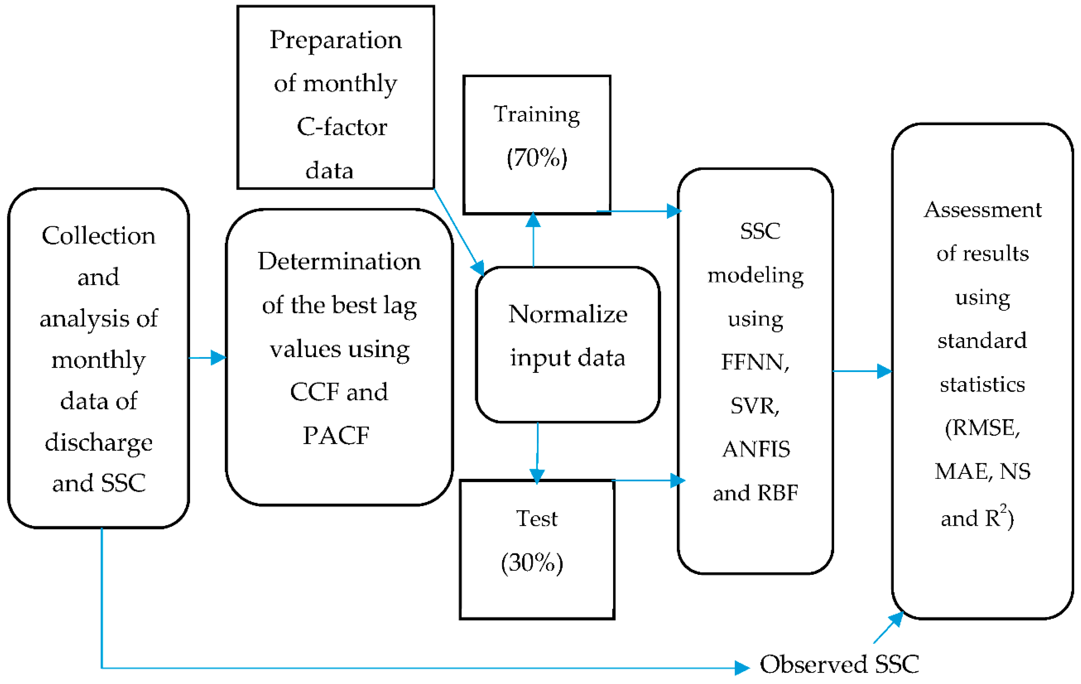
2. Materials and Methods

The general procedure used in this study includes the following steps: (1) the collection and analysis of monthly data; (2) the determination of the best lag times of inputs; (3) the normalization and then classification of the data into two groups of training and test sets; and (4) SSC modeling and model evaluation. Figure 1 illustrates the flowchart of the research methodology.

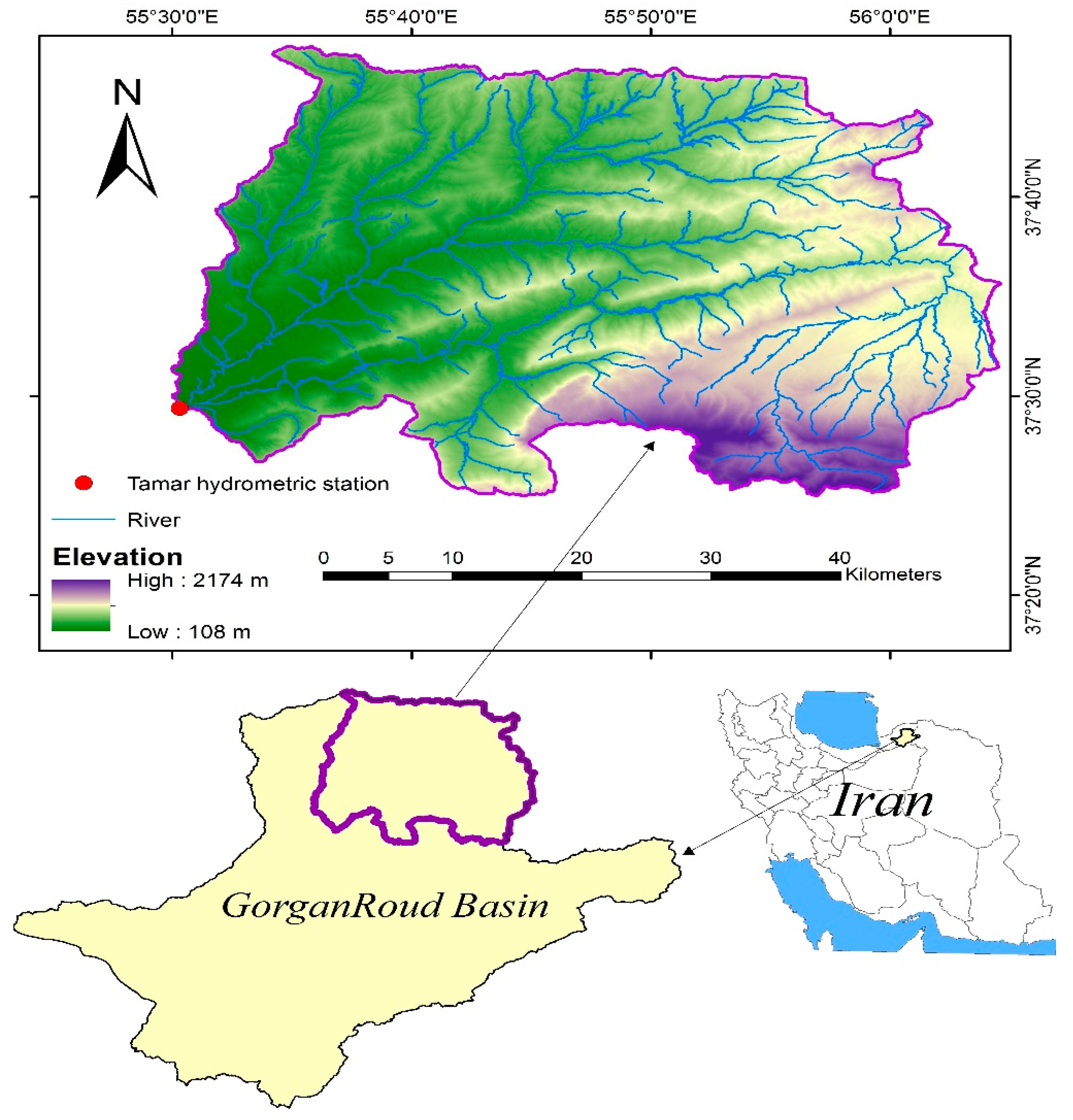
2.1. Study Area and Database

The Boostan Dam Watershed in Golestan Province, Iran, was selected to test the objectives of this study due to the availability of data and the absence of major abstractions or dams in the upstream reaches. This watershed has an area of 1533.3 km² and is located between 37°24′05″ and 37°47′33″ north latitude and 54°29′30″ and 56°05′35″ east longitude (Figure 2). The region has an average annual rainfall of 483 mm, an average annual temperature of 17.8 °C, relative humidity of 68.5%, an average slope gradient of 23%, and the minimum, maximum, and average elevations of 108, 2174, and 753 m a.s.l., respectively.

To conduct this research, the monthly flow discharge and SSC at the catchment outlet (Tamar Hydrometric Station) from April 2000 to September 2013 (comprising 162 datasets) were collected. The NDVI data of the relevant period were obtained from the MODIS/MCD43A4_006_NDVI product available at https://explorer.earthengine.google.com/, accessed on 20 September 2022; this product with a resolution of 500 × 500 m is generated from the MODIS/006/MCD43A4 surface reflectance composites. Then, the time series data were investigated to ensure they were continuous (without gaps). Finally, the dataset was classified into two groups: 70% of the total data were selected for the training phase, and the remaining 30% were selected for the test phase. The statistical parameters for the training and test datasets, the total datasets of discharge, SSC, and the C-factor were calculated and are presented in

Table 1. Statistical parameters of monthly SSC, discharge, and C-factor for the Boostan Dam Watershed ¹.

Variable	Statistical Parameter	Boostan Dam Watershed
		Training (70%)	Test (30%)	Total Data
	$\left(n\right)$	114	48	162
SSC (mg/L)	Period (m/y)	4/2000–9/2009	10/2009–9/2013	4/2000–9/2013
	$x_{min}$	0.01	0.24	0.01
	$x_{max}$	9259.15	299.63	9259.15
	$\overline{x}$	199.99	45.14	154.11
	${\sigma }_x$	940.87	68.59	792.28
	$G_1$	8.46	1.97	10.07
	${\beta }_2$	78.50	3.50	111.40
Q (m3/s)	$x_{min}$	0.00	0.01	0.00
	$x_{max}$	10.40	3.13	10.40
	$\overline{x}$	1.04	0.84	0.98
	${\sigma }_x$	1.11	0.75	1.02
	$G_1$	2.96	1.53	2.93
	${\beta }_2$	14.30	1.61	14.80
C	$x_{min}$	0.19	0.21	0.19
	$x_{max}$	0.43	0.41	0.43
	$\overline{x}$	0.33	0.34	0.33
	${\sigma }_x$	0.05	0.04	0.05
	$G_1$	−0.86	−1.30	−0.98
	${\beta }_2$	0.25	1.38	0.50

Note: ¹ SSC is suspended sediment concentration, Q is flow discharge, C is C-factor in RUSLE model, (n) is number of data, $x_{min}$ is the minimum value of the data, $x_{max}$ is the maximum value of the data, $\overline{x}$ is the mean of the data, ${\sigma }_x$ is the standard deviation,$G_1$ is the skewness, and ${\beta }_2$ is kurtosis.

. Very small and very large values of SSC and high skewness complicated the modeling process and yielded low model performance in the Boostan Dam Watershed.

2.2. C-Factor

The cover-management factor (C-factor) of the RUSLE model indicates the relationship between soil loss in an area with specific vegetation cover and management and bare areas. It reflects the effect of management practices and land use changes on soil erosion [46]. The amount, type, and stage of the growth of vegetation cover directly impact the C-factor because vegetation cover dissipates the kinetic energy of rainfall before reaching the soil surface and decreases erosion [47]. In our study, we estimated the C-factor using the rescaled NDVI [46] as follows:

$$\mathrm{C}=(\frac{1-\mathrm{NDVI}}{2})$$

(1)

The C-factor values range from 0 to 1, where 0 indicates fully protected soil and dense vegetation cover, and 1 denotes bare soil.

To determine the monthly NDVI values, we used moderate-resolution imaging spectroradiometer (MODIS) satellite imagery. Considering that NDVI variation is quite low during each month, the images in the middle of the months without cloud cover were used for the monthly NDVI [48]. A survey of the NDVI values in this watershed during the 13-year period showed similar monthly patterns during the study years and temporal variations in the NDVI, which caused variations in the C-factor. The monthly C-factor time series compared with the monthly discharge data from 2000 to 2013 is shown in Figure 3.

2.3. Input Scenarios

We modeled SSC using six different scenarios: (1) only the discharge data, (2) only the SSC data, (3) combining the discharge and SSC data, (4) combining the discharge and C-factor data, (5) combining the SSC and C-factor data, and (6) combining the discharge, SSC, and C-factor data. Identifying the optimum lag values of input vectors using DD algorithms is an important step in the modeling process [49]. To address this problem and avoid trial-and-error assessment, statistical parameters, such as the cross-correlation function (CCF), which occurs in two different time series, and the partial autocorrelation function (PACF), which occurs in two same time series, were used [36]. Finally, to improve the analysis, two groups of input scenarios were established: (1) only the hydrological data (group 1) and (2) a combination of the hydrological and C-factor data (group 2) (

Table 2. Input and output scenarios.

Scenario Number	Group Name	Inputs	Output
1	Group 1	${\mathrm{Q}}_{\mathrm{t}}$	${\mathrm{SSC}}_{\mathrm{t}}$
2		${\mathrm{Q}}_{\mathrm{t}}{+\mathrm{Q}}_{\mathrm{t}-1}$	${\mathrm{SSC}}_{\mathrm{t}}$
3		${\mathrm{SSC}}_{\mathrm{t}-1}$	${\mathrm{SSC}}_{\mathrm{t}}$
4		${\mathrm{Q}}_{\mathrm{t}}{+\mathrm{SSC}}_{\mathrm{t}-1}$	${\mathrm{SSC}}_{\mathrm{t}}$
5		${\mathrm{Q}}_{\mathrm{t}}{+\mathrm{Q}}_{\mathrm{t}-1}{+\mathrm{SSC}}_{\mathrm{t}-1}$	${\mathrm{SSC}}_{\mathrm{t}}$
6	Group 2	${\mathrm{Q}}_{\mathrm{t}}{+\mathrm{C}}_{\mathrm{t}}$	${\mathrm{SSC}}_{\mathrm{t}}$
7		${\mathrm{Q}}_{\mathrm{t}}{+\mathrm{Q}}_{\mathrm{t}-1}{+\mathrm{C}}_{\mathrm{t}}$	${\mathrm{SSC}}_{\mathrm{t}}$
8		${\mathrm{SSC}}_{\mathrm{t}-1}{+\mathrm{C}}_{\mathrm{t}}$	${\mathrm{SSC}}_{\mathrm{t}}$
9		${\mathrm{Q}}_{\mathrm{t}}{+\mathrm{SSC}}_{\mathrm{t}-1}{+\mathrm{C}}_{\mathrm{t}}$	${\mathrm{SSC}}_{\mathrm{t}}$
10		${\mathrm{Q}}_{\mathrm{t}}{+\mathrm{Q}}_{\mathrm{t}-1}{+\mathrm{SSC}}_{\mathrm{t}-1}{+\mathrm{C}}_{\mathrm{t}}$	${\mathrm{SSC}}_{\mathrm{t}}$

).

2.4. Data Preprocessing

Basically, entering the raw data reduces the speed and accuracy of AI models. To avoid such problems, the conversion of the data in a specific range ensures that they receive the same attention within the network. In this study, all the input data were normalized in the range [0–1] using Equation (2) [50] before introduction to the network.

$${\mathrm{X}}_{\mathrm{norm}}=\frac{{\mathrm{X}}_{\mathrm{i}}-{\mathrm{X}}_{\min }}{{\mathrm{X}}_{\max }-{\mathrm{X}}_{\min }}$$

(2)

where ${\mathrm{X}}_{\min }$ and ${\mathrm{X}}_{\max }$ represent the minimum and maximum values among the original data, ${\mathrm{X}}_{\mathrm{i}}$ represents the original data, and ${\mathrm{X}}_{\mathrm{norm}}$ represents the normalized data.

2.5. Model Theory Background

2.5.1. Support Vector Regression (SVR)

The SVR model is a supervised learning algorithm, introduced by Vapnik et al. [51], which has been successfully applied in geoscience, water resources, and sediment load prediction [26,36,52]. SVR is a version of SVM that performs regression instead of classification and transforms the separator hyperplane in SVM into a data-fitting function. SVR uses the structural risk minimization (SRM) principle leading to an overall optimal response and elevating the power of the model [53]. The SVR algorithm uses different types of kernel functions (e.g., linear, nonlinear, polynomial, the radial basis function (RBF), sigmoid), among which the RBF kernel has better performance and has been used more than other kernel functions in sediment studies [36,54]. The SVR and RBF algorithms (Equations (3) and (4)) are as follows [55]:

$$y={\displaystyle \sum }_{\mathrm{i}=1}^{\mathrm{n}}\left({\alpha }_i^{+}-{\alpha }_i^{-}\right)k\left(\mathrm{x},{\mathrm{x}}_{\mathrm{i}}\right)+b$$

(3)

$${\mathrm{K}(\mathrm{x},\mathrm{x}}_{\mathrm{i}})=\exp (\frac{-\left|\right|\mathrm{x}-{\mathrm{x}}_{\mathrm{i}}\left|\right|{}^2}{{2\mathsf{\sigma }}^2})$$

(4)

where y is the output, b is the bias term, α is the Lagrange multiplier, k(x,x_i) is the kernel function in which the RBF function is considered, and $\left(\mathsf{\sigma }\right)$ is the width of the Gaussian kernel function.

2.5.2. Adaptive Neuro-Fuzzy Inference System (ANFIS)

The ANFIS model uses a combination of an artificial neural network and fuzzy logic algorithms to design a nonlinear mapping between the input and output vectors [56]. The most common type of fuzzy inference system that can be applied in an adaptive network is the Takagi–Sugeno fuzzy system, the output of which is a linear function with its parameters determined by using a combination of the least square and backpropagation gradient descent methods. In general, the structure of the ANFIS model consists of 5 layers. The first layer is the input nodes, which determine the degree of the membership of each input according to its membership function. The second layer is the rule nodes; each node in this layer calculates the degree of the activity of a rule. The third layer is the average nodes, in which the normalized weight is calculated. The fourth layer is the consequent nodes, and the fifth layer is the output nodes [57]. To generate fuzzy rules, there are two methods: grid partitioning and subtractive fuzzy clustering. Grid partitioning is usually applied when there are few input variables, as in our study [58].

2.5.3. Feed-Forward Neural Network (FFNN)

ANNs are promising and efficient tools for modeling hydrological processes due to their ability to identify complex nonlinear relationships [24,46,59,60,61]. We used a widely recommended feed-forward artificial neural network model for time series simulation [36]. This network comprises the input, hidden, and output layers, and each layer consists of neurons that connect proximate layers, and there is no connection between the neurons within each layer [62]. The optimal number of neurons in the hidden layer was selected through trial and error. To train the network (i.e., weighting adjustment), we used a backpropagation mechanism based on a gradient scheme to decrease the error between the modeled and observed data [63]. Among the variants of the backpropagation training scheme, the Levenberg–Marquardt algorithm was applied, which is widely used due to its high speed in the training of neural networks [64].

2.5.4. Radial Basis Function (RBF)

The RBF Network, originally proposed by Broomhead and Lowe [65], is another type of artificial neural network with three layers (i.e., input, hidden, and output layers) which has been successfully applied in nonlinear system modeling such as the prediction of sediment transport [66,67,68]. In this type of ANN, the inputs from the input layer are mapped to each of the hidden units, and the hidden layer units perform nonlinear conversion operations without changing weights and parameters. To use the RBF networks, it is necessary to define the functions and number of neurons in the hidden layer, as well as the training algorithm to find the network parameters. Various activation functions have been proposed for the hidden layer of the RBF network [69]. One of the most widely used activation functions is the Gaussian function [70]. The training process includes the determination of the hidden layer weight, the standard deviation of the hidden layer neurons, and the output layer weight. The K-mean classification algorithm [69] and the gradient descent backpropagation method were used to determine the weights of the hidden layer and the connection weights between the hidden layer and the output layer, respectively.

2.6. Model Evaluation

We applied four different standard statistics, namely the coefficient of determination (R²), the root mean square error (RMSE), the mean absolute error (MAE), and the Nash–Sutcliffe efficiency coefficient (NS), to evaluate the performance of the various models during the training and test phases [24]:

$$\mathrm{RMSE}=\sqrt{\frac{1}{\mathrm{n}}{\displaystyle \sum }_{\mathrm{i}=1}^{\mathrm{n}}{\left({\mathrm{O}}_{\mathrm{i}}-{\mathrm{M}}_{\mathrm{i}}\right)}^2}$$

(5)

$$\mathrm{MAE}=\frac{{{\displaystyle \sum }}_{\mathrm{i}=1}^{\mathrm{n}}\left|{\mathrm{O}}_{\mathrm{i}}-{\mathrm{M}}_{\mathrm{i}}\right|}{\mathrm{n}}$$

(6)

$$\mathrm{NS}=1-\frac{{{\displaystyle \sum }}_{\mathrm{i}=1}^{\mathrm{n}}{\left({\mathrm{O}}_{\mathrm{i}}-{\mathrm{M}}_{\mathrm{i}}\right)}^2}{{{\displaystyle \sum }}_{\mathrm{i}=1}^{\mathrm{n}}{\left({\mathrm{O}}_{\mathrm{i}}-\overline{\mathrm{O}}\right)}^2}$$

(7)

$${\mathrm{R}}^2={\left[\frac{{{\displaystyle \sum }}_{\mathrm{i}=1}^{\mathrm{n}}\left({\mathrm{O}}_{\mathrm{i}}-\overline{\mathrm{O}}\right)\left({\mathrm{M}}_{\mathrm{i}}-\overline{\mathrm{M}}\right)}{\sqrt{{{\displaystyle \sum }}_{\mathrm{i}=1}^{\mathrm{n}}{\left({\mathrm{O}}_{\mathrm{i}}-\overline{\mathrm{O}}\right)}^2}\sqrt{{{\displaystyle \sum }}_{\mathrm{i}=1}^{\mathrm{n}}{\left({\mathrm{M}}_{\mathrm{i}}-\overline{\mathrm{M}}\right)}^2}}\right]}^2$$

(8)

where O_i and M_i are the observed and modeled SSC values, respectively; $\overline{\mathrm{O}}$ and $\overline{\mathrm{M}}$ are the averages of the observed and modeled SSC values; and n is the number of data (i.e., the number of the training and test data). The RMSE and MAE describe the difference between the observed and modeled data in the units of the variable. The RMSE and MAE vary between 0 and +∞, where lower RMSE and MAE values represent higher model performance, and their optimal value is zero [71]. The NS varies between −∞ and 1, and R² varies between 0 and 1. The closer the NS and R² values are to 1, the better the model prediction power [24].

3. Results and Discussion

3.1. Results of the Best Lag Times for Inputs

In this study, we applied the CCF and PACF to the training dataset to select the most highly correlated antecedent discharges and SSCs with the SSCs of each month in the Boostan Dam Watershed. Applying the CCF for the relationship between the monthly SSC and monthly discharge (with 6-month time lags) showed that SSC was highly correlated with discharge for the same month, followed by the discharge of the previous month (

Table 3. Cross-correlation between monthly SSC and discharge data with 5% significance limits and partial autocorrelation for monthly SSC data with 5% significance limits for Boostan Dam Watershed.

Lag	Cross-Correlation	Partial Autocorrelation
0	0.87	-
1	0.19	0.21
2	0.09	0.01
3	0.01	−0.03
4	−0.08	−0.14
5	−0.10	−0.15
6	−0.01	−0.03

). The PACF showed that the highest correlation occurred between the monthly SSC and the SSC of the previous month (Table 3). Finally, based on our analysis of the previously mentioned functions and using the relevant variables, 10 different input scenarios (Table 2) were developed and tested in each of the FFNN, ANFIS, RBF, and SVR models.

3.2. Results of Optimal Structure for Different Models

In AI models, there are parameters whose changes will influence the performance of the algorithms. In our study, to achieve the optimal network design and improve the SSC estimates, we applied a trial-and-error technique, and the optimal values of model parameters in all the scenarios were adjusted according to the lowest RMSE. The final optimal structures of the FFNN, SVR, ANFIS, and RBF models are shown for all the groups in

Table 4. Optimal structure of FFNN, RBF, ANFIS, and SVR models for different inputs ².

Scenario Number	FFNN	RBF		ANFIS		SVR
	No. HN	$\mathit{\sigma }$	No. HN	No. MF	MF	$\mathit{\sigma }$	C	ε
1	5	0.3	20	3	Gaussian-2	0.17	5	0.001
2	7	0.2	15	5	Gaussian	0.13	5	0.001
3	4	0.5	16	3	Gaussian-2	0.17	1	0.1
4	8	0.4	18	4	Bell	0.15	10	0.001
5	8	0.3	21	4	Gaussian-2	0.16	10	0.001
6	6	0.1	16	6	Gaussian	0.15	2.5	0.1
7	8	0.4	19	5	Gaussian-2	0.19	2	0.01
8	7	0.3	18	5	Bell	0.17	5	0.01
9	10	0.2	20	4	Gaussian-2	0.17	10	0.0001
10	10	0.7	16	4	Gaussian	0.21	10	0.0001

Note: ² No. HN is number of hidden neurons, No. MF is number of membership function, MF is membership function, $\mathsf{\sigma }$ is width of the Gaussian function, C is cost of constraint violation, and ε is error insensitive zone.

.

In FFNN, to determine the appropriate number of neurons in the hidden layer, the trial-and-error method was used (see Table 4); 4 to 10 neurons in this layer were selected for the training of the network. The activation functions used for the hidden and output layers were a combination of sigmoid functions since these functions are efficient for extrapolating the data beyond the training range [24]. Additionally, in the feed-forward neural network backpropagation mechanism, the Levenberg–Marquardt algorithm and the epoch 100 were used for training the network. For the RBF model, a trial-and-error technique was used to assess the width parameter (spread constant) and the appropriate number of hidden neurons (Table 4). The results showed that the RBF required more neurons in the hidden layer to achieve a minimum error compared with the FFNN. The Gaussian and linear functions were used for the hidden and output layers, respectively. The ANFIS model based on the Takagi–Sugeno fuzzy inference system was developed. To train the system, a hybrid algorithm was used due to its high efficiency in training the ANFIS systems [72], and for data-fuzzifying and fuzzy rule extraction, a grid partitioning method was used. For each input scenario, different input membership functions (e.g., trapezoidal, Gaussian, Gaussian-2, triangular, bell, pi) and output membership functions (e.g., linear, constant) were tested. The results, based on trial and error, indicated the superiority of Gaussian, Gaussian-2, and bell for the input membership function in estimating the monthly SSC. Additionally, the optimum number of membership functions for each input scenario was identified (Table 4). The SVR model was tested using the RBF kernel. The optimal values for model parameters (namely, σ, C, and ε) were obtained for all the input scenarios through trial and error and considering the lowest RMSE values (Table 4).

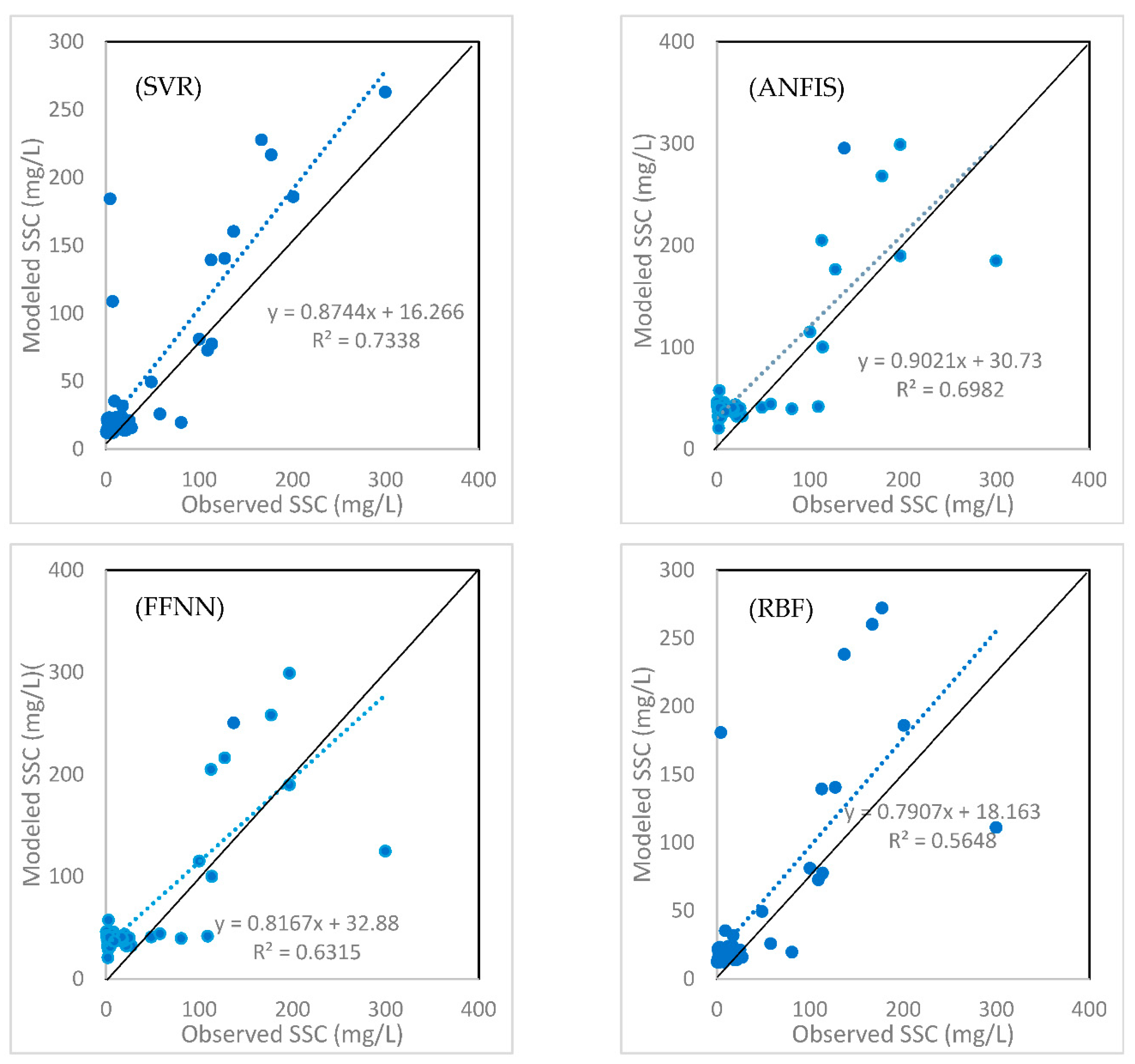
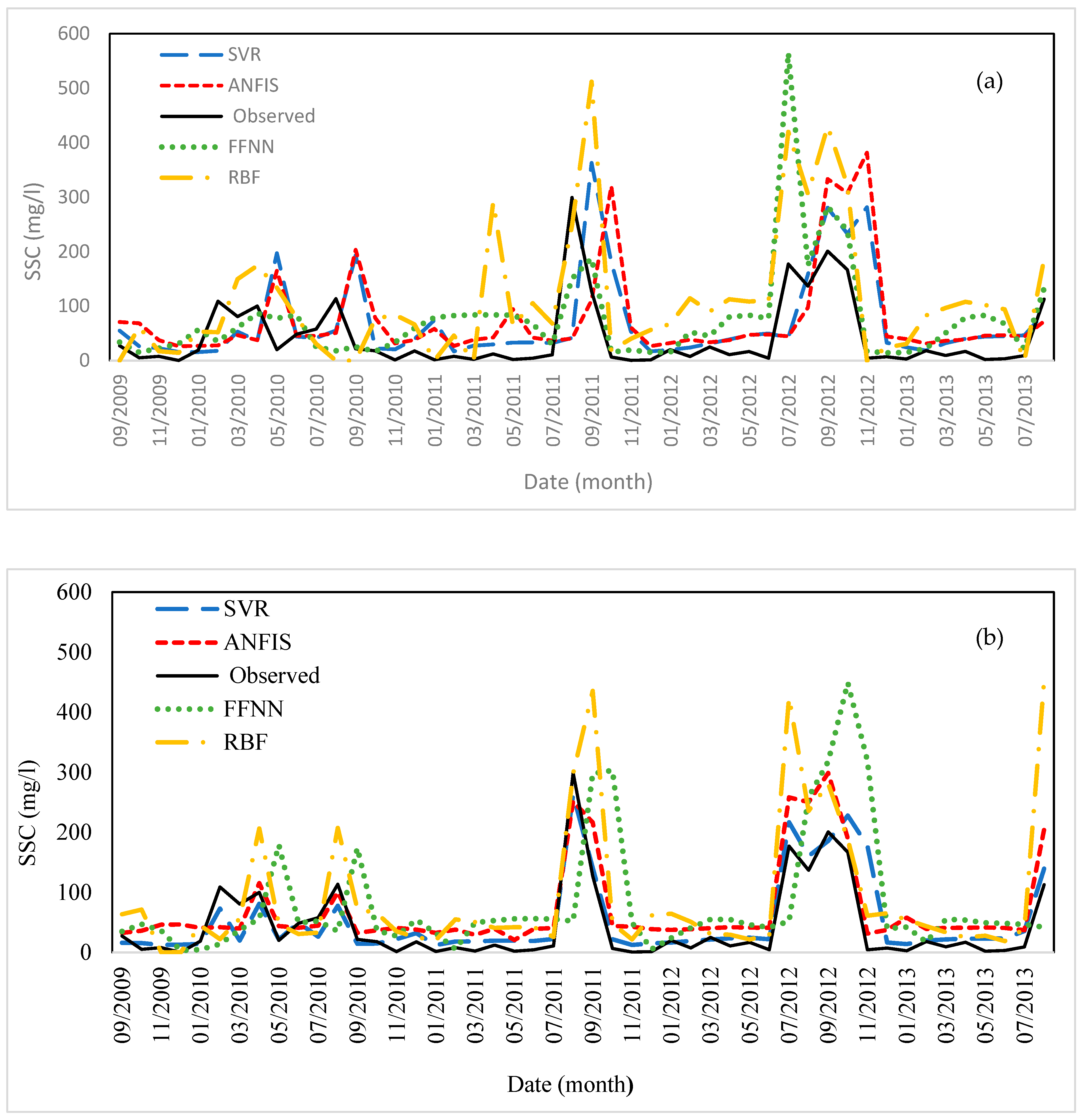
3.3. Evaluations and Results of Different Models and Input Scenarios for Estimating SSC

According to the results from the different input scenarios in the SVR model (

Table 5. Results of monthly SSC modeling by SVR with different input patterns during training and test phases.

Input Patterns	Training				Test
	RMSE (mg/L)	NS	MAE (mg/L)	R2	RMSE (mg/L)	NS	MAE (mg/L)	R2
${\mathrm{Q}}_{\mathrm{t}}$	214.01	0.66	92.58	0.70	203.19	0.56	99.11	0.66
${\mathrm{Q}}_{\mathrm{t}}{+\mathrm{Q}}_{\mathrm{t}-1}$	221.52	0.64	93.09	0.73	223.24	0.54	106.63	0.63
${\mathrm{SSC}}_{\mathrm{t}-1}$	439.23	0.35	201.63	0.38	444.11	0.29	222.71	0.33
${\mathrm{Q}}_{\mathrm{t}}{+\mathrm{SSC}}_{\mathrm{t}-1}$	199.32	0.68	88.71	0.76	211.96	0.55	99.76	0.63
${\mathrm{Q}}_{\mathrm{t}}{+\mathrm{Q}}_{\mathrm{t}-1}{+\mathrm{SSC}}_{\mathrm{t}-1}$	195.51	0.72	79.50	0.79	201.85	0.61	96.92	0.66
${\mathrm{Q}}_{\mathrm{t}}{+\mathrm{C}}_{\mathrm{t}}$	181.81	0.71	77.41	0.80	199.64	0.65	91.76	0.69
${\mathrm{Q}}_{\mathrm{t}}{+\mathrm{Q}}_{\mathrm{t}-1}{+\mathrm{C}}_{\mathrm{t}}$	178.65	0.74	72.31	0.83	191.54	0.69	84.39	0.71
${\mathrm{SSC}}_{\mathrm{t}-1}{+\mathrm{C}}_{\mathrm{t}}$	297.96	0.39	166.35	0.49	317.68	0.35	177.19	0.44
${\mathrm{Q}}_{\mathrm{t}}{+\mathrm{SSC}}_{\mathrm{t}-1}{+\mathrm{C}}_{\mathrm{t}}$	168.95	0.83	64.45	0.90	183.12	0.71	78.39	0.76
${\mathrm{Q}}_{\mathrm{t}}{+\mathrm{Q}}_{\mathrm{t}-1}{+\mathrm{SSC}}_{\mathrm{t}-1}{+\mathrm{C}}_{\mathrm{t}}$	159.71	0.89	61.56	0.92	171.82	0.73	73.67	0.78

), the best input scenario for estimating the monthly SSC during the test phase of the first group (i.e., only considering the hydrological data), was ${\mathrm{Q}}_{\mathrm{t}}{+\mathrm{Q}}_{\mathrm{t}-1}{+\mathrm{SSC}}_{\mathrm{t}-1}$ with the RMSE, MAE, NS, and R² of 201.8 mg/L, 96.9 mg/L, 0.61, and 0.66, respectively, and in the second group (i.e., a combination of hydrological inputs and the C-factor) was ${\mathrm{Q}}_{\mathrm{t}}{+\mathrm{Q}}_{\mathrm{t}-1}{+\mathrm{SSC}}_{\mathrm{t}-1}{+\mathrm{C}}_{\mathrm{t}}$ with the RMSE, MAE, NS and R² of 171.8 mg/L, 73.6 mg/L, 0.73, and 0.78, respectively. Therefore, ${\mathrm{Q}}_{\mathrm{t}}{+\mathrm{Q}}_{\mathrm{t}-1}{+\mathrm{SSC}}_{\mathrm{t}-1}{+\mathrm{C}}_{\mathrm{t}}$ was the best input combination among all of these. Assessing the results of the best input scenario (compared with the best scenario using only hydrological inputs) showed that using the C-factor as an input improved the NS by 16.4% and R² by 15.4% and decreased the RMSE by 17.5% and MAE by 31.5%.

In the ANFIS model (

Table 6. Results of monthly SSC modeling by ANFIS with different input patterns during training and test phases.

Input Patterns	Training				Test
	RMSE (mg/L)	NS	MAE (mg/L)	R2	RMSE (mg/L)	NS	MAE (mg/L)	R2
${\mathrm{Q}}_{\mathrm{t}}$	237.37	0.60	99.11	0.65	239.66	0.53	121.07	0.54
${\mathrm{Q}}_{\mathrm{t}}{+\mathrm{Q}}_{\mathrm{t}-1}$	232.07	0.61	100.15	0.70	241.33	0.49	118.17	0.59
${\mathrm{SSC}}_{\mathrm{t}-1}$	509.11	0.28	209.29	0. 35	592.23	0.21	276.91	0.30
${\mathrm{Q}}_{\mathrm{t}}{+\mathrm{SSC}}_{\mathrm{t}-1}$	222.59	0.63	96.47	0.74	231.88	0.50	108.09	0.61
${\mathrm{Q}}_{\mathrm{t}}{+\mathrm{Q}}_{\mathrm{t}-1}{+\mathrm{SSC}}_{\mathrm{t}-1}$	201.15	0.67	92.53	0.78	227.95	0.55	101.05	0.65
${\mathrm{Q}}_{\mathrm{t}}{+\mathrm{C}}_{\mathrm{t}}$	196.87	0.69	81.68	0.79	225.05	0.57	99.08	0.65
${\mathrm{Q}}_{\mathrm{t}}{+\mathrm{Q}}_{\mathrm{t}-1}{+\mathrm{C}}_{\mathrm{t}}$	193.94	0.71	79.20	0.81	221.88	0.61	94.91	0.68
${\mathrm{SSC}}_{\mathrm{t}-1}{+\mathrm{C}}_{\mathrm{t}}$	310.39	0.37	178.74	0.44	369.28	0.34	198.32	0.40
${\mathrm{Q}}_{\mathrm{t}}{+\mathrm{SSC}}_{\mathrm{t}-1}{+\mathrm{C}}_{\mathrm{t}}$	177.90	0.81	67.95	0.89	198.95	0.70	79.24	0.73
${\mathrm{Q}}_{\mathrm{t}}{+\mathrm{Q}}_{\mathrm{t}-1}{+\mathrm{SSC}}_{\mathrm{t}-1}{+\mathrm{C}}_{\mathrm{t}}$	183.87	0.75	73.06	0.87	216.41	0.67	91.20	0.71

), the best input combination for estimating the monthly SSC during the test phase in the first group was ${\mathrm{Q}}_{\mathrm{t}}{+\mathrm{Q}}_{\mathrm{t}-1}{+\mathrm{SSC}}_{\mathrm{t}-1}$ with the RMSE, MAE, NS, and R² of 227.9 mg/L, 101 mg/L, 0.55, and 0.65, respectively, and in the second group, it was ${\mathrm{Q}}_{\mathrm{t}}{+\mathrm{SSC}}_{\mathrm{t}-1}{+\mathrm{C}}_{\mathrm{t}}$ with the RMSE, MAE, NS and R² of 198.9 mg/L, 79.2 mg/L, 0.70, and 0.73, respectively. An evaluation of the results of the best input combination (i.e., ${\mathrm{Q}}_{\mathrm{t}}{+\mathrm{SSC}}_{\mathrm{t}-1}{+\mathrm{C}}_{\mathrm{t}}$) compared with the best scenario using only hydrological inputs (i.e.,${\mathrm{Q}}_{\mathrm{t}}{+\mathrm{Q}}_{\mathrm{t}-1}{+\mathrm{SSC}}_{\mathrm{t}-1}$) showed that including the C-factor improved the NS by 21.4% and R² by 10.9% and decreased the RMSE by 14.6% and MAE by 27.5%.

Our evaluation of the results of the different input scenarios in the FFNN and RBF models (

Table 7. Results of monthly SSC modeling by FFNN with different input patterns during training and test phases.

Input Patterns	Training				Test
	RMSE (mg/L)	NS	MAE (mg/L)	R2	RMSE (mg/L)	NS	MAE (mg/L)	R2
${\mathrm{Q}}_{\mathrm{t}}$	257.37	0.41	129.17	0.47	269.66	0.38	131.57	0.44
${\mathrm{Q}}_{\mathrm{t}}{+\mathrm{Q}}_{\mathrm{t}-1}$	241.11	0.50	120.13	0.59	253.33	0.43	128.06	0.51
${\mathrm{SSC}}_{\mathrm{t}-1}$	571.11	0.19	224.02	0. 25	634.23	0.11	299.98	0.17
${\mathrm{Q}}_{\mathrm{t}}{+\mathrm{SSC}}_{\mathrm{t}-1}$	212.39	0.55	106.47	0.67	242.88	0.48	117.19	0.56
${\mathrm{Q}}_{\mathrm{t}}{+\mathrm{Q}}_{\mathrm{t}-1}{+\mathrm{SSC}}_{\mathrm{t}-1}$	207.15	0.59	98.53	0.71	229.95	0.52	99.29	0.61
${\mathrm{Q}}_{\mathrm{t}}{+\mathrm{C}}_{\mathrm{t}}$	208.87	0.57	101.68	0.68	239.05	0.47	109.16	0.51
${\mathrm{Q}}_{\mathrm{t}}{+\mathrm{Q}}_{\mathrm{t}-1}{+\mathrm{C}}_{\mathrm{t}}$	201.94	0.61	99.20	0.71	231.88	0.51	98.91	0.58
${\mathrm{SSC}}_{\mathrm{t}-1}{+\mathrm{C}}_{\mathrm{t}}$	333.19	0.30	191.41	0.39	401.28	0.24	208.21	0.34
${\mathrm{Q}}_{\mathrm{t}}{+\mathrm{SSC}}_{\mathrm{t}-1}{+\mathrm{C}}_{\mathrm{t}}$	186.90	0.74	74.95	0.79	201.95	0.63	85.24	0.69
${\mathrm{Q}}_{\mathrm{t}}{+\mathrm{Q}}_{\mathrm{t}-1}{+\mathrm{SSC}}_{\mathrm{t}-1}{+\mathrm{C}}_{\mathrm{t}}$	196.62	0.67	81.22	0.77	226.51	0.59	97.30	0.66

and

Table 8. Results of monthly SSC modeling by RBF with different input patterns during training and test phases.

Input Patterns	Training				Test
	RMSE (mg/L)	NS	MAE (mg/L)	R2	RMSE (mg/L)	NS	MAE (mg/L)	R2
${\mathrm{Q}}_{\mathrm{t}}$	267.37	0.31	139.17	0.43	269.66	0.28	146.57	0.34
${\mathrm{Q}}_{\mathrm{t}}{+\mathrm{Q}}_{\mathrm{t}-1}$	254.11	0.41	130.13	0.46	273.33	0.32	139.06	0.41
${\mathrm{SSC}}_{\mathrm{t}-1}$	593.11	0.11	244.02	0. 19	664.23	0.09	301.98	0.13
${\mathrm{Q}}_{\mathrm{t}}{+\mathrm{SSC}}_{\mathrm{t}-1}$	231.39	0.49	126.47	0.51	252.88	0.39	137.19	0.45
${\mathrm{Q}}_{\mathrm{t}}{+\mathrm{Q}}_{\mathrm{t}-1}{+\mathrm{SSC}}_{\mathrm{t}-1}$	216.15	0.53	116.53	0.61	240.95	0.43	121.29	0.51
${\mathrm{Q}}_{\mathrm{t}}{+\mathrm{C}}_{\mathrm{t}}$	228.87	0.50	124.68	0.59	243.05	0.42	131.16	0.48
${\mathrm{Q}}_{\mathrm{t}}{+\mathrm{Q}}_{\mathrm{t}-1}{+\mathrm{C}}_{\mathrm{t}}$	211.94	0.55	119.20	0.64	239.88	0.46	128.91	0.54
${\mathrm{SSC}}_{\mathrm{t}-1}{+\mathrm{C}}_{\mathrm{t}}$	351.19	0.25	198.41	0.31	452.28	0.19	226.21	0.27
${\mathrm{Q}}_{\mathrm{t}}{+\mathrm{SSC}}_{\mathrm{t}-1}{+\mathrm{C}}_{\mathrm{t}}$	204.90	0.61	98.95	0.69	235.95	0.52	108.24	0.59
${\mathrm{Q}}_{\mathrm{t}}{+\mathrm{Q}}_{\mathrm{t}-1}{+\mathrm{SSC}}_{\mathrm{t}-1}{+\mathrm{C}}_{\mathrm{t}}$	198.12	0.65	89.13	0.75	231.01	0.56	99.89	0.65

, respectively) showed that, in the first group, ${\mathrm{Q}}_{\mathrm{t}}{+\mathrm{Q}}_{\mathrm{t}-1}{+\mathrm{SSC}}_{\mathrm{t}-1}$ was the best input combination. Additionally, ${\mathrm{Q}}_{\mathrm{t}}{+\mathrm{SSC}}_{\mathrm{t}-1}{+\mathrm{C}}_{\mathrm{t}}$ with RMSE = 201.95 mg/L, MAE = 85.24 mg/L, NS = 0.63, and R² = 0.69, and ${\mathrm{Q}}_{\mathrm{t}}{+\mathrm{Q}}_{\mathrm{t}-1}{+\mathrm{SSC}}_{\mathrm{t}-1}{+\mathrm{C}}_{\mathrm{t}}$ with RMSE = 231.01 mg/L, MAE = 99.89 mg/L, NS = 0.56, and R² = 0.65 were the best input scenario among all the 10 different input scenarios for SSC estimation using the FFNN and RBF models, respectively. Adding the C-factor was effective in improving model performance; the NS increased by 17.5% and 23.2%, R² increased by 11.6% and 21.5%), the RMSE decreased by 13.8% and 4.3%, and the MAE decreased by 16.5% and 21.4% for the FFNN and RBF models, respectively.

The SVR model showed superior performance (NS = 0.73), followed by ANFIS (NS = 0.70), FFNN (NS = 0.63), and RBF (NS = 0.56) (see Table 5, Table 6, Table 7 and Table 8). The accuracy of the SVR model was about 4.1%, 13.7%, and 23.3% higher than that of ANFIS, FFNN, and RBF for SSC estimation, respectively. Based on the NS metrics, the SVR and ANFIS models showed good performance (0.65<NS ≤ 0.75), and the FFNN and RBF models had lesser performance but were satisfactory (0.55<NS ≤ 0.65). However, based on the RMSE observation–standard deviation ratio (RSR) (i.e., RMSE/SD_obs), the results were not satisfactory. Because, RMSE values less than half of the standard deviation (SD) of the observed data is considered low and satisfactory [71,73,74].

Comparing the results of the best input scenarios for groups 1 and 2 showed that the inclusion of the C-factor improved model performance (based on the NS metric) by 16.4%, 21.4%, 17.5%, and 23.2% for SVR, ANFIS, FFNN, and RBF, respectively. Additionally, to assess the efficiency of the developed models, the correlations between the observed and modeled SSC during the test phase are presented for the best input patterns of the SVR, ANFIS, FFNN, and RBF models (Figure 4). These comparisons showed that the RBF model had the lowest correlation among all the tested models, and the SVR model had the best correlation.

Comparing the observed versus the simulated SSC using the models (i.e., MLP, ANFIS, RBF, and SVR) for the best input scenarios in groups 1 and 2 showed good agreement between the observed and simulated SSC using the SVR model, followed by ANFIS, FFNN, and RBF models, respectively (Figure 5). However, these models could not simulate the peak values accurately, a typical problem in modeling [7,75]. In general, all four models overestimated SSC, similar to findings by Choubin et al. [32]. Additionally, these graphs confirmed the better agreement between the observed and modeled SSC values during the test period when the C-factor was used along with hydrological inputs than when only using hydrological inputs.

Based on our findings, generally, the SVR model provided more accurate results in all the cases with lower error values and higher NS and R² than the ANFIS, FFNN, and RBF models. Other studies have confirmed the superiority of the SVR over ANN, ANFIS, and RBF models for suspended sediment estimation [5,32,36,38,76,77]. In fact, the application of the structural risk minimization (SRM) principle in the SVR modeling process, which minimizes the upper limit of the expected error, equips the SVR model with a promising tool for generalization, while the application of the empirical risk minimization (ERM) principle in the ANN modeling process minimizes the training data error [53]. The ANFIS model was the next best-performing model for estimating SSC. The better performance of the ANFIS model, compared with FFNN, indicates that the combination of fuzzy logic with neural network analysis increases model efficiency in estimating sediment similar to other findings [28,49,78]. The FFNN model performs better than RBF. The weak performance of RBF for estimating SSC is likely because this network divides the patterns before creating the mapping and creates a nonlinear mapping for each class, causing poorer performance of the network. Research also shows that RBFs often perform better in classification problems, and ANNs are more suitable for curve fitting [79].

Our results showed that only using discharge as a model input does not provide accurate estimates of the suspended sediment load because other variables control the supply and transport of the suspended sediment load (e.g., rainfall, land use, the sediment from antecedent flooding, watershed physiography, anthropogenic change) [26]. Similarly, Rodríguez-Blanco et al. [80] indicated that the flow discharge explained only 19% of the variation in SSL. Additionally, Nhu et al. [9] and Salih et al. [81] confirmed that discharge alone does not accurately estimate SSC.

Based on our results from the Boostan Dam Watershed, incorporating the discharge and SSC data of the previous month increased model accuracy compared with using only the discharge during the same month. This denotes the importance of antecedent values of these data in the suspended sediment generation process [32]. Moreover, the results achieved from all the applied models showed that including the C-factor along with hydrological inputs led to greater efficiency of the models; without the C-factor, even the best combination of the discharge and SSC data produced a higher modeling error than when the C-factor was included.

To assess the performance of the models, in addition to a good fit, an accurate simulation of the peak SSC values is important. To check this, we assessed the relative error of the best model for predicting the peak SSC ${(\%\mathrm{RE}}_{\mathrm{P}})$ using only hydrological variables and using both hydrological variables and the C-factor as follows [82]:

$${\%\mathrm{RE}}_{\mathrm{P}}=\frac{{\mathrm{M}}_{\mathrm{P}}-{\mathrm{O}}_{\mathrm{P}}}{{\mathrm{O}}_{\mathrm{P}}}\times 100$$

(9)

where ${\mathrm{O}}_{\mathrm{P}}$ and ${\mathrm{M}}_{\mathrm{P}}$ are the observed and modeled peak SSC, respectively. The results indicated that the peak SSC values were more accurately predicted when adding the C-factor to hydrological inputs in all four models (

Table 9. Assessment of models based on relative error in peak SSC for the best model using only hydrological variables and the best model using hydrological variables along with C-factor for Boostan Dam Watershed.

Model	The Best Input Pattern in Group 1	%REp	The Best Input Pattern in Group 1	%REp
SVR	${\mathrm{Q}}_{\mathrm{t}}{+\mathrm{Q}}_{\mathrm{t}-1}{+\mathrm{SSC}}_{\mathrm{t}-1}$	21.13	${\mathrm{Q}}_{\mathrm{t}}{+\mathrm{Q}}_{\mathrm{t}-1}{+\mathrm{SSC}}_{\mathrm{t}-1}{+\mathrm{C}}_{\mathrm{t}}$	−12.21
ANFIS	${\mathrm{Q}}_{\mathrm{t}}{+\mathrm{Q}}_{\mathrm{t}-1}{+\mathrm{SSC}}_{\mathrm{t}-1}$	27.39	${\mathrm{Q}}_{\mathrm{t}}{+\mathrm{Q}}_{\mathrm{t}-1}{+\mathrm{SSC}}_{\mathrm{t}-1}$	−12.28
FFNN	${\mathrm{Q}}_{\mathrm{t}}{+\mathrm{Q}}_{\mathrm{t}-1}{+\mathrm{SSC}}_{\mathrm{t}-1}$	70.56	${\mathrm{Q}}_{\mathrm{t}}{+\mathrm{SSC}}_{\mathrm{t}-1}{+\mathrm{C}}_{\mathrm{t}}$	49.94
RBF	${\mathrm{Q}}_{\mathrm{t}}{+\mathrm{Q}}_{\mathrm{t}-1}{+\mathrm{SSC}}_{\mathrm{t}-1}$	88.89	${\mathrm{Q}}_{\mathrm{t}}{+\mathrm{Q}}_{\mathrm{t}-1}{+\mathrm{SSC}}_{\mathrm{t}-1}{+\mathrm{C}}_{\mathrm{t}}$	51.28

).

This poor simulation of peak values can arise from several sources. First, only a few SSC samples were collected at high flows, causing a bias in the representation of the peak conditions within our database (e.g., Ziegler et al. [83]). Secondly, the uncertainties of the suspended sediment data can contribute to poor performance [26]. A third reason is that the rainfall data were not used, and the peak of SSC data is affected by intense rainfall [83]. The choice of the data range during the training phase can also affect the peak flow prediction [36]. Finally, geomorphic perturbations in the watershed (e.g., landslides, bank collapse) can affect the peak sediment fluxes [7,83].

Moreover, the utilization of climatic variables, (e.g., rainfall, temperature, potential evapotranspiration) [33,34] and hydrogeomorphic variables (e.g., the index of sediment connectivity) [35] along with the inputs used in this study can most likely improve the estimation of SSC. Overall, our results showed that, for an accurate estimation of SSC, in addition to the modeling tool, acceptable and effective input data are necessary for building an efficient model [26,32].

4. Conclusions

The determination of soil loss within a basin is not simple because soil erosion and sediment transport are complex hydrodynamic phenomena that are influenced by various dynamic and static parameters. On the other hand, an accurate estimation of SSL/SSC is a key step in river basin and water resource management, including the design of hydraulic structures. This study was carried out to improve SSC estimation using the FFNN, SVR, RBF, and ANFIS models and different input patterns for the Boostan Dam Watershed in Iran. To construct an effective input scenario, we added the C-factor of the RUSLE along with hydrological variables to estimate the monthly SSC and found that this strategy improved model performance, as reflected the soil cover dynamics. Given that field surveys for collecting information on parameters such as the C-factor are time-consuming, using remote sensing combined with GIS can efficiently supply such data to the employed models. Our results showed that to accurately estimate SSC, in addition to the model type and structure, finding the relevant variables is necessary. Our findings are summarized as follows:

• The use of the C-factor in models elevated the performance of SSC modeling;
• Using only the discharge values of the same month did not accurately estimate SSC; other variables such as the monthly discharge with a 1-month time lag and the SSC within a 1-month time lag played important roles in this process;
• The SVR models performed best, followed by the ANFIS, FFNN, and RBF models, respectively. Based on the NS metric, the SVR and ANFIS models had good levels of performance, and the FFNN and RBF models had a lesser but satisfactory performance;
• The best input combination for models was determined as ${\mathrm{Q}}_{\mathrm{t}}{+\mathrm{Q}}_{\mathrm{t}-1}{+\mathrm{SSC}}_{\mathrm{t}-1}{+\mathrm{C}}_{\mathrm{t}}$;
• To construct an effective input scenario for estimating the monthly SSC, using the C-factor of the RUSLE as an input along with hydrological variables is important;
• Given that our optimization of the model parameters was accomplished through trial and error, we recommend surveying the meta-heuristic optimization algorithms, including the multi-objective and single-objective algorithms, for selecting those parameters that increase the accuracy of SSC estimation.

References

1. Ziegler, A.D.; Sidle, R.C.; Phang, V.X.; Wood, S.H.; Tantasirin, C. Bedload transport in SE Asian streams—Uncertainties and implications for reservoir management. Geomorphology 2014, 227, 31–48. [Google Scholar] [CrossRef]
2. Zhu, Y.-M.; Lu, X.; Zhou, Y. Suspended sediment flux modeling with artificial neural network: An example of the Longchuanjiang River in the Upper Yangtze Catchment, China. Geomorphology 2007, 84, 111–125. [Google Scholar] [CrossRef]
3. Sidle, R.C.; Milner, A.M. Stream development in Glacier Bay National Park, Alaska, USA. Arct. Alp. Res. 1989, 21, 350–363. [Google Scholar] [CrossRef]
4. Pektaş, A.O.; Doğan, E. Prediction of bed load via suspended sediment load using soft computing methods. Geofizika 2015, 32, 27–46. [Google Scholar] [CrossRef]
5. Buyukyildiz, M.; Kumcu, S.Y. An estimation of the suspended sediment load using adaptive network based fuzzy inference system, support vector machine and artificial neural network models. Water Resour. Manag. 2017, 31, 1343–1359. [Google Scholar] [CrossRef]
6. Sarkar, A.; Sharma, N.; Singh, R. Sediment Runoff Modelling Using ANNs in an Eastern Himalayan Basin, India. In River System Analysis and Management; Springer: Berlin/Heidelberg, Germany, 2017; pp. 73–82. [Google Scholar]
7. Khosravi, K.; Golkarian, A.; Melesse, A.M.; Deo, R.C. Suspended sediment load modeling using advanced hybrid Rotation Forest based Elastic Network approach. J. Hydrol. 2022, 610, 127963. [Google Scholar] [CrossRef]
8. Rajaee, T.; Mirbagheri, S.A.; Zounemat-Kermani, M.; Nourani, V. Daily suspended sediment concentration simulation using ANN and neuro-fuzzy models. Sci. Total Environ. 2009, 407, 4916–4927. [Google Scholar] [CrossRef] [PubMed]
9. Nhu, V.-H.; Khosravi, K.; Cooper, J.R.; Karimi, M.; Kisi, O.; Pham, B.T.; Lyu, Z. Monthly suspended sediment load prediction using artificial intelligence: Testing of a new random subspace method. Hydrol. Sci. J. 2020, 65, 2116–2127. [Google Scholar] [CrossRef]
10. Khosravi, K.; Golkarian, A.; Booij, M.J.; Barzegar, R.; Sun, W.; Yaseen, Z.M.; Mosavi, A. Improving daily stochastic streamflow prediction: Comparison of novel hybrid data-mining algorithms. Hydrol. Sci. J. 2021, 66, 1457–1474. [Google Scholar] [CrossRef]
11. Srinivasulu, S.; Jain, A. A comparative analysis of training methods for artificial neural network rainfall–runoff models. Appl. Soft Comput. 2006, 6, 295–306. [Google Scholar] [CrossRef]
12. Dastorani, M.T.; Wright, N.G. A hydrodynamic/neural network approach for enhanced river flow prediction. Int. J. Civ. Eng. 2004, 2, 141–148. [Google Scholar]
13. Wu, C.; Chau, K.W. Rainfall–runoff modeling using artificial neural network coupled with singular spectrum analysis. J. Hydrol. 2011, 399, 394–409. [Google Scholar] [CrossRef]
14. Dastorani, M.T.; Moghadamnia, A.; Piri, J.; Rico-Ramirez, M. Application of ANN and ANFIS models for reconstructing missing flow data. Environ. Monit. Assess. 2010, 166, 421–434. [Google Scholar] [CrossRef] [PubMed]
15. Dastorani, M.T.; Talebi, A.; Dastorani, M. Using neural networks to predict runoff from ungauged catchments. Asian J. Appl. Sci. 2010, 3, 399–410. [Google Scholar] [CrossRef]
16. Dastorani, M.T.; Mahjoobi, J.; Talebi, A.; Fakhar, F. Application of Machine Learning Approaches in Rainfall-Runoff Modeling (Case Study: Zayandeh_Rood Basin in Iran). Civ. Eng. Infrastruct. J. 2018, 51, 293–310. [Google Scholar]
17. Moatamednia, M.; Nohegar, A.; Malekian, A.; Asadi, H.; Tavasoli, A.; Safari, M.; Karimi, K. Daily river flow forecasting in a semi-arid region using twodatadriven. Desert 2015, 20, 11–21. [Google Scholar]
18. Dastorani, M.T.; Koochi, J.S.; Darani, H.S.; Talebi, A.; Rahimian, M. River instantaneous peak flow estimation using daily flow data and machine-learning-based models. J. Hydroinf. 2013, 15, 1089–1098. [Google Scholar] [CrossRef]
19. Moghaddam, H.K.; Moghaddam, H.K.; Kivi, Z.R.; Bahreinimotlagh, M.; Alizadeh, M.J. Developing comparative mathematic models, BN and ANN for forecasting of groundwater levels. Groundw. Sustain. Dev. 2019, 9, 100237. [Google Scholar] [CrossRef]
20. Yoon, H.; Hyun, Y.; Ha, K.; Lee, K.-K.; Kim, G.-B. A method to improve the stability and accuracy of ANN-and SVM-based time series models for long-term groundwater level predictions. Comput. Geosci. 2016, 90, 144–155. [Google Scholar] [CrossRef]
21. Dastorani, M.T.; Afkhami, H.; Sharifidarani, H.; Dastorani, M. Application of ANN and ANFIS models on dryland precipitation prediction (case study: Yazd in central Iran). J. Appl. Sci. 2010, 10, 2387–2394. [Google Scholar] [CrossRef]
22. Dastorani, M.T.; Afkhami, H. Application of artificial neural networks on drought prediction in Yazd (Central Iran). Desert 2011, 16, 39–48. [Google Scholar]
23. Melesse, A.; Ahmad, S.; McClain, M.; Wang, X.; Lim, Y. Suspended sediment load prediction of river systems: An artificial neural network approach. Agric. Water Manag. 2011, 98, 855–866. [Google Scholar] [CrossRef]
24. Zounemat-Kermani, M.; Kişi, Ö.; Adamowski, J.; Ramezani-Charmahineh, A. Evaluation of data driven models for river suspended sediment concentration modeling. J. Hydrol. 2016, 535, 457–472. [Google Scholar] [CrossRef]
25. Talebi, A.; Mahjoobi, J.; Dastorani, M.T.; Moosavi, V. Estimation of suspended sediment load using regression trees and model trees approaches (Case study: Hyderabad drainage basin in Iran). ISH J. Hydraul. Eng. 2017, 23, 212–219. [Google Scholar] [CrossRef]
26. Asadi, H.; Dastorani, M.T.; Sidle, R.C.; Shahedi, K. Improving Flow Discharge-Suspended Sediment Relations: Intelligent Algorithms versus Data Separation. Water 2021, 13, 3650. [Google Scholar] [CrossRef]
27. Roushangar, K.; Koosheh, A. Evaluation of GA-SVR method for modeling bed load transport in gravel-bed rivers. J. Hydrol. 2015, 527, 1142–1152. [Google Scholar] [CrossRef]
28. Riahi-Madvar, H.; Seifi, A. Uncertainty analysis in bed load transport prediction of gravel bed rivers by ANN and ANFIS. Arab. J. Geosci. 2018, 11, 688. [Google Scholar] [CrossRef]
29. Asheghi, R.; Hosseini, S.A. Prediction of bed load sediments using different artificial neural network models. Front. Struct. Civ. Eng. 2020, 14, 374–386. [Google Scholar] [CrossRef]
30. Yang, C.T.; Marsooli, R.; Aalami, M.T. Evaluation of total load sediment transport formulas using ANN. Int. J. Sediment Res. 2009, 24, 274–286. [Google Scholar] [CrossRef]
31. Noori, R.; Ghiasi, B.; Salehi, S.; Esmaeili Bidhendi, M.; Raeisi, A.; Partani, S.; Meysami, R.; Mahdian, M.; Hosseinzadeh, M.; Abolfathi, S. An Efficient Data Driven-Based Model for Prediction of the Total Sediment Load in Rivers. Hydrology 2022, 9, 36. [Google Scholar] [CrossRef]
32. Choubin, B.; Darabi, H.; Rahmati, O.; Sajedi-Hosseini, F.; Kløve, B. River suspended sediment modelling using the CART model: A comparative study of machine learning techniques. Sci. Total Environ. 2018, 615, 272–281. [Google Scholar] [CrossRef]
33. Gao, G.; Ning, Z.; Li, Z.; Fu, B. Prediction of long-term inter-seasonal variations of streamflow and sediment load by state-space model in the Loess Plateau of China. J. Hydrol. 2021, 600, 126534. [Google Scholar] [CrossRef]
34. Banadkooki, F.B.; Ehteram, M.; Ahmed, A.N.; Teo, F.Y.; Ebrahimi, M.; Fai, C.M.; Huang, Y.F.; El-Shafie, A. Suspended sediment load prediction using artificial neural network and ant lion optimization algorithm. Environ. Sci. Pollut. Res. 2020, 27, 38094–38116. [Google Scholar] [CrossRef]
35. Asadi, H.; Shahedi, K.; Sidle, R.C.; Kalami Heris, S.M. Prediction of Suspended Sediment Using Hydrologic and Hydrogeomorphic Data within Intelligence Models. Iran-Water Resour. Res. 2019, 15, 105–119. [Google Scholar]
36. Kumar, D.; Pandey, A.; Sharma, N.; Flügel, W.-A. Daily suspended sediment simulation using machine learning approach. Catena 2016, 138, 77–90. [Google Scholar] [CrossRef]
37. Khan, M.Y.A.; Tian, F.; Hasan, F.; Chakrapani, G.J. Artificial neural network simulation for prediction of suspended sediment concentration in the River Ramganga, Ganges Basin, India. Int. J. Sediment Res. 2019, 34, 95–107. [Google Scholar] [CrossRef]
38. Chiang, J.-L.; Tsai, K.-J.; Chen, Y.-R.; Lee, M.-H.; Sun, J.-W. Suspended sediment load prediction using support vector machines in the Goodwin Creek experimental watershed. In Proceedings of the EGU General Assembly Conference Abstracts, Vienna, Austria, 3–8 April 2011; p. 5285. [Google Scholar]
39. Kisi, O.; Haktanir, T.; Ardiclioglu, M.; Ozturk, O.; Yalcin, E.; Uludag, S. Adaptive neuro-fuzzy computing technique for suspended sediment estimation. Adv. Eng. Softw. 2009, 40, 438–444. [Google Scholar] [CrossRef]
40. Khosravi, K.; Mao, L.; Kisi, O.; Yaseen, Z.M.; Shahid, S. Quantifying hourly suspended sediment load using data mining models: Case study of a glacierized Andean catchment in Chile. J. Hydrol. 2018, 567, 165–179. [Google Scholar] [CrossRef]
41. Rezaei, K.; Pradhan, B.; Vadiati, M.; Nadiri, A.A. Suspended sediment load prediction using artificial intelligence techniques: Comparison between four state-of-the-art artificial neural network techniques. Arab. J. Geosci. 2021, 14, 1–13. [Google Scholar] [CrossRef]
42. Kumar, A.; Tripathi, V.K. Capability assessment of conventional and data-driven models for prediction of suspended sediment load. Environ. Sci. Pollut. Res. 2022, 29, 50040–50058. [Google Scholar] [CrossRef]
43. Renard, K.G. Predicting Soil Erosion by Water: A Guide to Conservation Planning with the Revised Universal Soil Loss Equation (RUSLE); United States Government Printing: Washington, DC, USA, 1997. [Google Scholar]
44. Kastridis, A.; Stathis, D.; Sapountzis, M.; Theodosiou, G. Insect outbreak and long-term post-fire effects on soil erosion in mediterranean suburban forest. Land 2022, 11, 911. [Google Scholar] [CrossRef]
45. Ferreira, C.S.; Seifollahi-Aghmiuni, S.; Destouni, G.; Ghajarnia, N.; Kalantari, Z. Soil degradation in the European Mediterranean region: Processes, status and consequences. Sci. Total Environ. 2021, 805, 150106. [Google Scholar] [CrossRef] [PubMed]
46. Durigon, V.; Carvalho, D.; Antunes, M.; Oliveira, P.; Fernandes, M. NDVI time series for monitoring RUSLE cover management factor in a tropical watershed. Int. J. Remote Sens. 2014, 35, 441–453. [Google Scholar] [CrossRef]
47. Ghosal, K.; Das Bhattacharya, S. A review of RUSLE model. J. Indian Soc. Remote Sens. 2020, 48, 689–707. [Google Scholar] [CrossRef]
48. Asadi, H.; Shahedi, K.; Jarihani, B.; Sidle, R.C. Rainfall-runoff modelling using hydrological connectivity index and artificial neural network approach. Water 2019, 11, 212. [Google Scholar] [CrossRef] [Green Version]
49. Kumar, A.; Kumar, P.; Singh, V.K. Evaluating different machine learning models for runoff and suspended sediment simulation. Water Resour. Manag. 2019, 33, 1217–1231. [Google Scholar] [CrossRef]
50. Vafakhah, M. Comparison of cokriging and adaptive neuro-fuzzy inference system models for suspended sediment load forecasting. Arab. J. Geosci. 2013, 6, 3003–3018. [Google Scholar] [CrossRef]
51. Vapnik, V. The nature of statistical learning theory. IEEE Trans. Neural Netw. 1995, 195, 5. [Google Scholar]
52. Kazemi, M.S.; Banihabib, M.E.; Soltani, J. A hybrid SVR-PSO model to predict concentration of sediment in typical and debris floods. Earth Sci. Inform. 2021, 14, 365–376. [Google Scholar] [CrossRef]
53. Cristianini, N.; Shawe-Taylor, J. An Introduction to Support Vector Machines and Other Kernel-Based Learning Methods; Cambridge University Press: Cambridge, UK, 2000. [Google Scholar]
54. Wang, H.; Xu, D. Parameter selection method for support vector regression based on adaptive fusion of the mixed kernel function. J. Control Sci. Eng. 2017, 2017. [Google Scholar] [CrossRef]
55. Chen, S.-T.; Yu, P.-S. Pruning of support vector networks on flood forecasting. J. Hydrol. 2007, 347, 67–78. [Google Scholar] [CrossRef]
56. Jang, J.-S. ANFIS: Adaptive-network-based fuzzy inference system. IEEE Trans. Syst. Man Cybern. 1993, 23, 665–685. [Google Scholar] [CrossRef]
57. Chen, S.H.; Lin, Y.H.; Chang, L.C.; Chang, F.J. The strategy of building a flood forecast model by neuro-fuzzy network. Hydrol. Processes: Int. J. 2006, 20, 1525–1540. [Google Scholar] [CrossRef]
58. Jang, J.-S.R.; Sun, C.-T. Neuro-fuzzy modeling and control. Proc. IEEE 1995, 83, 378–406. [Google Scholar] [CrossRef]
59. Pumo, D.; Francipane, A.; Lo Conti, F.; Arnone, E.; Bitonto, P.; Viola, F.; La Loggia, G.; Noto, L. The SESAMO early warning system for rainfall-triggered landslides. J. Hydroinformatics 2016, 18, 256–276. [Google Scholar] [CrossRef]
60. Nourani, V.; Kisi, Ö.; Komasi, M. Two hybrid artificial intelligence approaches for modeling rainfall–runoff process. J. Hydrol. 2011, 402, 41–59. [Google Scholar] [CrossRef]
61. Goyal, M.K.; Bharti, B.; Quilty, J.; Adamowski, J.; Pandey, A. Modeling of daily pan evaporation in sub tropical climates using ANN, LS-SVR, Fuzzy Logic, and ANFIS. Expert Syst. Appl. 2014, 41, 5267–5276. [Google Scholar] [CrossRef]
62. Kim, T.-W.; Valdés, J.B. Nonlinear model for drought forecasting based on a conjunction of wavelet transforms and neural networks. J. Hydrol. Eng. 2003, 8, 319–328. [Google Scholar] [CrossRef]
63. Hagan, M.T.; Menhaj, M.B. Training feedforward networks with the Marquardt algorithm. IEEE Trans. Neural Netw. 1994, 5, 989–993. [Google Scholar] [CrossRef]
64. Huang, G.-B.; Zhu, Q.-Y.; Siew, C.-K. Extreme learning machine: Theory and applications. Neurocomputing 2006, 70, 489–501. [Google Scholar] [CrossRef]
65. Broomhead, D.S.; Lowe, D. Radial Basis Functions, Multi-Variable Functional Interpolation and Adaptive Networks; Royal Signals and Radar Establishment Malvern: UK, 1988. [Google Scholar]
66. Alp, M.; Cigizoglu, H.K. Suspended sediment load simulation by two artificial neural network methods using hydrometeorological data. Environ. Model. Softw. 2007, 22, 2–13. [Google Scholar] [CrossRef]
67. Ebtehaj, I.; Bonakdari, H.; Zaji, A.H. An expert system with radial basis function neural network based on decision trees for predicting sediment transport in sewers. Water Sci. Technol. 2016, 74, 176–183. [Google Scholar] [CrossRef] [PubMed]
68. Isa, M.M.M. Comparative study of MLP and RBF neural networks for estimation of suspended sediments in Pari River, Perak. Res. J. Appl. Sci. Eng. Technol. 2014, 7, 3837–3841. [Google Scholar]
69. Haykin, S. Neural Networks, a comprehensive foundation, Prentice-Hall Inc. Up. Saddle River New Jersey 1999, 7458, 161–175. [Google Scholar]
70. Sudheer, K.; Jain, S. Radial basis function neural network for modeling rating curves. J. Hydrol. Eng. 2003, 8, 161–164. [Google Scholar] [CrossRef]
71. Moriasi, D.N.; Arnold, J.G.; van Liew, M.W.; Bingner, R.L.; Harmel, R.D.; Veith, T.L. Model evaluation guidelines for systematic quantification of accuracy in watershed simulations. Trans. ASABE 2007, 50, 885–900. [Google Scholar] [CrossRef]
72. Jang, J.-S.R.; Sun, C.-T.; Mizutani, E. Neuro-fuzzy and soft computing-a computational approach to learning and machine intelligence [Book Review]. IEEE Trans. Autom. Control 1997, 42, 1482–1484. [Google Scholar] [CrossRef]
73. Kastridis, A.; Theodosiou, G.; Fotiadis, G. Investigation of Flood Management and Mitigation Measures in Ungauged NATURA Protected Watersheds. Hydrology 2021, 8, 170. [Google Scholar] [CrossRef]
74. Singh, J.; Knapp, H.V.; Arnold, J.G.; Demissie, M. Hydrological modeling of the Iroquois river watershed using HSPF and SWAT. JAWRA J. Am. Water Resour. Assoc. 2005, 41, 343–360. [Google Scholar] [CrossRef]
75. Sichingabula, H.M. Factors controlling variations in suspended sediment concentration for single-valued sediment rating curves, Fraser River, British Columbia, Canada. Hydrol. Processes 1998, 12, 1869–1894. [Google Scholar] [CrossRef]
76. Lafdani, E.K.; Nia, A.M.; Ahmadi, A. Daily suspended sediment load prediction using artificial neural networks and support vector machines. J. Hydrol. 2013, 478, 50–62. [Google Scholar] [CrossRef]
77. Kisi, O.; Dailr, A.H.; Cimen, M.; Shiri, J. Suspended sediment modeling using genetic programming and soft computing techniques. J. Hydrol. 2012, 450, 48–58. [Google Scholar] [CrossRef]
78. Samet, K.; Hoseini, K.; Karami, H.; Mohammadi, M. Comparison between soft computing methods for prediction of sediment load in rivers: Maku dam case study. Iran. J. Sci. Technol. Trans. Civ. Eng. 2019, 43, 93–103. [Google Scholar] [CrossRef]
79. Pantazi, X.; Moshou, D.; Bochtis, D. Chapter 2—Artificial intelligence in agriculture. In Intelligent Data Mining and Fusion Systems in Agriculture; Pantazi, X.E., Moshou, D., Bochtis, D., Eds.; Springer: Berlin/Heidelberg, Germany, 2020; pp. 17–101. [Google Scholar]
80. Rodríguez-Blanco, M.; Taboada-Castro, M.; Palleiro, L.; Taboada-Castro, M. Temporal changes in suspended sediment transport in an Atlantic catchment, NW Spain. Geomorphology 2010, 123, 181–188. [Google Scholar] [CrossRef]
81. Salih, S.Q.; Sharafati, A.; Khosravi, K.; Faris, H.; Kisi, O.; Tao, H.; Ali, M.; Yaseen, Z.M. River suspended sediment load prediction based on river discharge information: Application of newly developed data mining models. Hydrol. Sci. J. 2020, 65, 624–637. [Google Scholar] [CrossRef]
82. Hosseini, S.M.; Mahjouri, N. Integrating support vector regression and a geomorphologic artificial neural network for daily rainfall-runoff modeling. Appl. Soft Comput. 2016, 38, 329–345. [Google Scholar] [CrossRef]
83. Ziegler, A.D.; Benner, S.G.; Tantasirin, C.; Wood, S.H.; Sutherland, R.A.; Sidle, R.C.; Jachowski, N.; Nullet, M.A.; Xi, L.X.; Snidvongs, A. Turbidity-based sediment monitoring in northern Thailand: Hysteresis, variability, and uncertainty. J. Hydrol. 2014, 519, 2020–2039. [Google Scholar] [CrossRef]
Figure 1. Flowchart of research methodology.
Water 14 03011 g001
Figure 2. Location of the Tamar Hydrometric Station and drainage network map of Boostan Dam Watershed.
Water 14 03011 g002
Figure 3. Monthly C-factor and flow discharge (Q) time series plot for Boostan Dam Watershed (2000–2013).
Water 14 03011 g003
Figure 4. Scatter plots of the observed and estimated SSC based on the best input scenario during test phase for SVR, ANFIS, FFNN, and RBF models.
Water 14 03011 g004
Figure 5. Time series plots of the observed and estimated SSC based on the best input scenarios of group 1 (a) and group 2 (b) during test phase.
Water 14 03011 g005