Trend Test for Hydrological and Climatic Time Series Considering the Interaction of Trend and Autocorrelations

Abstract

The Mann–Kendall (MK) test was widely used to detect significant trends in hydrologic and climate time series (HCTS), but it cannot deal with significant autocorrelations in HCTS. To solve this problem, the modified MK (MMK) test and the over-whitening (OW) operation were successively proposed. However, there are still limitations for these two methods, especially for the OW operation. When an HCTS has unknown interaction scenarios of trends and autocorrelations, it is obviously unclear which of these two methods will perform better in the trend test. Additionally, the trend test is always accompanied by an autocorrelations test. In the dual test, it is also unknown how the significance level affects the accuracy of the trend test. To address these issues, this study first proposes a strategy of adding an outer loop to modify the OW-operation-based trend test. Then, two simulation experiments are designed to evaluate the performances of MMK-test-based and OW-operation-based methods, and the influence of the significance level on the trend test is analyzed. Moreover, six HCTSs in the Huaihe River basin are taken as examples to examine the consistence and difference of trend test results of these two methods. Results show that: (1) previous OW operations still have the risk of misjudging trends in the presence of significant autocorrelations, and the proposed strategy is necessary and effective to modify the OW operation; (2) these two methods are similar in the accuracy of the trend test results, but they may also produce opposite results when determining whether a significant trend is a pseudo trend or not; and (3) at a given significance level α, the accuracy rates of two methods are always less than 1-α, and the accuracy rate of the trend test tends to decrease for short HCTSs and increase for long HCTSs as the significance level decreases. This study would provide a new perspective for the trend test of HCTS based on the MK test.

1. Introduction

With the intensification of global warming and human activities, changes in the hydrologic and climatic time series (HCTS) have shown significant non-stationarity in many regions around the world [1,2]. This situation has brought many new and unexpected challenges to social economics [3], people’s health and lifestyles [4,5], and wildlife survival [6], which have adapted to a relatively stationary climate environment in the past. Before taking active countermeasures, it is particularly important to identify the non-stationary change characteristics of hydrological and climatic time series [7,8].

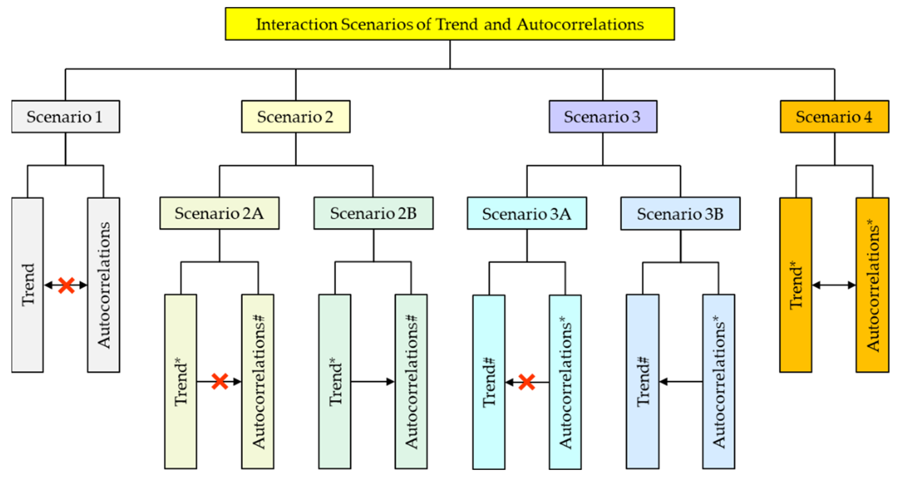
As a major manifestation of non-stationarity, trends embedded in various HCTSs have attracted extensive attention in the hydro-meteorological community [9,10]. The available research focuses mostly on how to accurately test the significance of HCTS trends in the presence of significant autocorrelations, which has a considerable impact on the trend test result [11,12]. As can be seen in Figure 1, there are four rough interaction scenarios (six detailed scenarios) of trends and autocorrelations for an HCTS. Specifically, Scenario 1 denotes that an HCTS has neither a significant trend nor significant autocorrelations. Scenario 2, which can be divided into two detailed scenarios, i.e., Scenarios 2A and 2B, shows that an HCTS has a significant trend but has no significant autocorrelations. In Scenario 2A, the significant trend does not cause significant pseudo autocorrelations; while in Scenario 2B, the significant trend leads to significant pseudo autocorrelations. Scenario 3 represents that an HCTS has significant autocorrelations but has no significant trend, which can also be decomposed into two detailed scenarios, i.e., Scenarios 3A and 3B. Scenario 3A is that the significant autocorrelations do not result in a significant pseudo trend. However, the significant autocorrelations give rise to a significant pseudo trend in Scenario 3B. Scenario 4 indicates that an HCTS has a significant trend and significant autocorrelations, which interact with each other. There is no doubt that the existence of six detailed interaction scenarios complicates the trend tests of various HCTS in the real world.

The Mann–Kendall (MK) test [13,14] is the most widely used non-parametric trend test method; it has no strict requirements on data distribution in an HCTS compared to other parametric trend test methods [15]. However, the MK test assumes that the data in a time series are independent, which is difficult to satisfy for an HCTS since it may have significant autocorrelations [12]. Without considering significant autocorrelations, the MK test may generate a false trend test result for a time series [11]. For example, as shown in Figure 2a, X1 and X2 are independent and dependent random time series, respectively. The two random time series have the same length, the same average value, and the same variance. Furthermore, the autocorrelation functions (ACFs) of X1 and X2 are shown in Figure 2b. One can see that the autocorrelation coefficients of X1 are insignificant at the 5% significance level, while R₁, R₁₂, and R₁₃ are significant for X2. At the 5% significance level, the MK test results show that X1 has an insignificant trend (p-value = 0.1006) while X2 has a significant trend (p-value = 0.0086). Apparently, the significant autocorrelations lead to a pseudo trend for X2. Therefore, eliminating the effect of significant autocorrelations is crucial to accurately determine the significance of trends in HCTS using the MK test. According to previous studies, this study summarized three general MK test-based trend test methods to eliminate the influence of autocorrelations, namely, the separation method [16,17,18], the implantation method [11,19], and the interference method [7,20].

The separation method is to separate the autocorrelation components from an HCTS of length n and then use the MK test to examine the trend of the residual components or bootstrapped time series. Von Storch (1995) [16] presented a pre-whitening operation to perform the MK test by removing serial correlation in an HCTS. Considering the possible damage of the pre-whitening operation to the real trends, Yue and Wang (2002) [17] further suggested a trend-free pre-whitening operation for the trend test on an HCTS. In addition, Noguchi et al. (2011) [18] proposed a sieve bootstrap approach that can be combined with the MK test for estimating and evaluating trends in HCTSs. Specifically, the sieve bootstrap approach extracts the autocorrelation components of an HCTS and obtains the residuals and then uses the resampled residuals as a noise to simulate many new bootstrapped time series. These bootstrapped time series, with an autocorrelation structure similar to that of the HCTS, can provide inference on the trend of the HCTS. Due to its simplicity, the separation method was used to test the trends of HCTSs in some regions [21,22]. Nevertheless, when the m-order (m is the maximum order of the autocorrelation coefficient, m < n) autocorrelation coefficient is significant, the exact autocorrelation components of the HCTS between t₀ (recording time of the first data) and t₀ + m−1 cannot be derived, resulting in a shorter length of the effective residuals. When the proportion of m in n is very large, the trend tests based on the separation method tend to be unreliable. In other words, the separation method is not suitable for the trend test on an HCTS with high-order autocorrelations.

The implantation method aims to modify the MK statistic by implanting the significant autocorrelation coefficients into the test statistic, thus, reducing the effect of autocorrelations [18]. Hammed and Rao (1998) [11] proposed a modified Mann–Kendall (MMK) test method by taking the influence of autocorrelations on the variance of an MK trend test statistic into account. To test the trend of persistent HCTS, Hammed (2009) [19] further developed a new MK test statistic and verified that it could be easily described by the Beta distribution. The implantation method such as the MMK test is popular in many studies because it takes higher-order autocorrelations into account [23,24]. However, the inaccurate estimation and test of higher-order autocorrelation coefficients of HCTSs may lead to failure of the trend test when using the implantation method.

Unlike the separation and implantation methods, the interference method aims to disrupt the serial correlation of an HCTS by superimposing a noise series on the HCTS, thus, rendering the HCTS into an independent series. Şen (2017) [7] designed an over-whitening (OW) operation to add a randomly generated Gaussian white noise to the standardized HCTS for the MK test. Şen (2017) [7] claimed that the OW operation does little damage to the true trend of original HCTS under the finite variance of white noise but did not provide an effective approach to determine the variance of white noise. In addition, randomly generated white noise with a specific variance may not succeed in disrupting the serial correlation in HCTS at once. Considering the two issues, Xie et al. (2022) [20] modified the OW operation in testing local trends of HCTSs. Specifically, they adopted a strategy of gradually increasing the white noise variance in small steps. However, white noise with sufficiently large variance may alter the significance of the trend in the HCTS. Thus, it is still an unsolved problem for the OW operation to ensure the reliability of the trend test results when continuously increasing the noise variance to destroy the autocorrelations.

Compared to the separation method, the implantation and interference methods have stronger applicability in testing trends of HCTSs with higher-order autocorrelations. For an HCTS with an unknown interaction scenario of trend and autocorrelations, both implantation and interference methods can be used to test the trend of the HCTS. In this case, which method performs better under the same significance level (α)? To the best of our knowledge, this question was not yet discussed in previous studies. In addition, the trend test is always accompanied by an autocorrelations test, and the significance level (e.g., α = 10%, 5% and 1%) is given before the trend and autocorrelations tests. For an HCTS with a certain length, it is still unclear how the significance level would affect the accuracy of the trend test in the joint test of trend and autocorrelations.

Therefore, using the MMK test and OW operation as representatives of the implantation and interference methods, respectively, this study aims to achieve the three following outcomes: (1) provide an effective strategy to achieve reliable trend test results for HCTS using the OW operation; (2) evaluate the performances of the MMK test and OW operation in testing trends in HCTSs; and (3) reveal the impact of the significance level on the trend test in HCTSs in different interaction scenarios.

2. Methods

2.1. Trend and Autocorrelations Analysis

2.1.1. MK Test and MMK Test

(1)

MK test

In the trend test of time series x(t) (t = 1, …, n), the MK test statistic (Z_MK) is given as:

$$Z_{\mathrm{MK}}=\{\begin{array}{l}\frac{S-1}{\sqrt{\mathrm{Var}\left(S\right)}}, \mathrm{if} S>0;\\ 0, \mathrm{if} S=0;\\ \frac{S+1}{\sqrt{\mathrm{Var}\left(S\right)}}, \mathrm{if} S<0.\end{array}$$

(1)

where:

$$\mathrm{Var}\left(S\right)=\frac{1}{18}\left[n\left(n-1\right)\left(2n+5\right)-{\displaystyle \sum _{i=1}^m{t}_i\left(t_i-1\right)\left(2t_i+5\right)}\right]$$

(2)

where Z_MK asymptotically follows the standard normal distribution with the increasing length (n) of the time series; S is the trend test statistic [11]; Var(S) denotes the variance of S considering ties in the time series; n is the length of the time series [19]; m denotes the number of tied values; and t_i is the number of ties for the ith value.

If the data in the time series are independent, the trend in the time series is significant and |Z_MK| is larger than Z_1−α/2, where Z_1−α/2 is the 1 − α/2 quantile of the standard normal distribution; otherwise, the trend is not significant.

(2)

MMK test

Taking significant high-order autocorrelations into account, the MMK test statistic (Z_MMK) is built as:

$$Z_{\mathrm{MMK}}=\frac{S}{\sqrt{\mu \cdot \mathrm{Var}\left(S\right)}}$$

(3)

where:

$$\mu =1+\frac{12}{n\left(n-1\right)\left(n-2\right)\pi }{\displaystyle \sum _{j=1}^{L_{\max }}\left[\left(n-j\right)\left(n-j-1\right)\left(n-j-2\right)\cdot \arcsin \left(\frac{{\rho }_j}{2}\right)\right]}$$

(4)

where Z_MMK asymptotically obeys the standard normal distribution [11,19]; μ is the correction factor of variance for the time series; ρ_j is the jth-order autocorrelation coefficient that is significant, and ρ_j = 0 if it is not significant; and L_max is the maximum integer, which is not larger than n/4, because the estimation of ρ_j tends to be more and more inaccurate with an increasing value of j [25].

When the time series has significant autocorrelations, the trend is significant if |Z_MMK| is more than Z_1−α/2; otherwise, it is not significant.

2.1.2. Autocorrelations Test

(1)

Single-order autocorrelation test

The ith-order autocorrelation coefficient (ρ_i) is estimated by Equation (5) for its small mean squared error [25]:

$$r_i=\frac{{\displaystyle \sum _{j=1}^{n-i}\left[x\left(j\right)-x_{\mathrm{a}}\right]\left[x\left(j+i\right)-x_{\mathrm{a}}\right]}}{{\displaystyle \sum _{k=1}^n{\left[x\left(k\right)-x_{\mathrm{a}}\right]}^2}}$$

(5)

where r_i is the estimator of ρ_i; and x_a is the average value of x(t).

The single-order autocorrelation test statistic [24] is expressed as:

$$Z_{\rho }\left(i\right)=\frac{1+\left(n-i\right)r_i}{\sqrt{n-i-1}}$$

(6)

where Z_ρ(i) is the test statistic that asymptotically obeys the standard normal distribution.

Under the significance level α, r_i (r_i ≤ n/4) is significant if |Z_ρ| is larger than Z_1−α/2; otherwise, r_i is not significant.

(2)

Overall test for high-order autocorrelations

The Box–Pierce test [26] and its modified version, the Ljung–Box test [27], are two commonly used high-order autocorrelation test methods. However, they do not perform as well as expected in testing for high-order autocorrelations because both neglect that the sum of sample autocorrelation function is a constant value [25,28]. Compared to the Box–Pierce and Ljung–Box tests, the quadratic sum test proposed by [28] is more effective in judging the existence of high-order autocorrelations. The test statistic (Q) of the quadratic sum test is given as:

$$Q={\displaystyle \sum _{i=1}^{n-1}{r}_i^2}$$

(7)

$$Q_{\alpha }=\frac{1}{2}+\frac{2}{\pi }{\cot }^{-1}\left\{a\cdot \exp \left[b\cdot {\left({\log }_{10}n\right)}^c\right]\right\}$$

(8)

where Q_α is an empirical critical value to examine the existence of high-order autocorrelations under the significance level α [28]; cot⁻¹ denotes the inverse function of cotangent function; and a, b, and c are three parameters depending on the significance level α.

There are high-order autocorrelations in x(t) if Q is larger than Q_α; otherwise, x(t) has no high-order autocorrelations. Note that the quadratic sum test cannot judge the significance of the first-order autocorrelation. To test the global autocorrelations for a sample time series, the first-order autocorrelation is tested by Equation (6), and high-order autocorrelations are tested with Equations (7) and (8).

2.1.3. De-Trending Operation

Autocorrelation components should be stationary. Hammed and Rao (1998) [11] and Yue and Wang (2002) [17] suggested that it is necessary to remove the trend component from an original HCTS before testing the significance of autocorrelations for the HCTS. Xie et al. (2020) [28] found that eliminating linear trends was less detrimental to the original autocorrelation function of a sample time series than eliminating nonlinear trends. In the study, the Sen’s trend estimator is employed to estimate the linear trend of a time series [29], which is given by:

$$x’\left(t\right)=k\cdot t$$

(9)

where:

$$k=\mathrm{med}\left(\frac{x_j-x_i}{j-i}\right)$$

(10)

where x’(t) represents the trend component estimated by the Sen’s trend estimator; k is the trend slope; and med denotes the median operator.

Then, the de-trended component of x(t) is given as:

$$y\left(t\right)=x\left(t\right)-x’\left(t\right)$$

(11)

where y(t) is the de-trended component.

2.1.4. OW Operation

Once the original time series x(t) has significant autocorrelations, it is first standardized as follows:

$$z\left(t\right)=\frac{x\left(t\right)-x_a}{\sqrt{\mathrm{Var}\left[x\left(t\right)\right]}}$$

(12)

where z(t) is the standardized time series; and Var[x(t)] denotes the variance of x(t).

The OW operation [7] is formulated as:

$$u\left(t\right)=z\left(t\right)+\epsilon \left(t\right)$$

(13)

where u(t) denotes the over-whitened time series; and ε(t) is the Gaussian white noise series with the variance of γ.

For u(t), the trend slope k_u can be estimated by Equation (10) if the global autocorrelations are not significant and the trend is significant. According to Xie et al. (2022) [20], the trend slope k_x for x(t) can be derived by:

$$k_x=k_u\cdot \sqrt{\mathrm{Var}\left[x\left(t\right)\right]}$$

(14)

2.2. Trend Tests Based on the MMK Test and OW Operation

2.2.1. Trend Test Based on the MMK Test

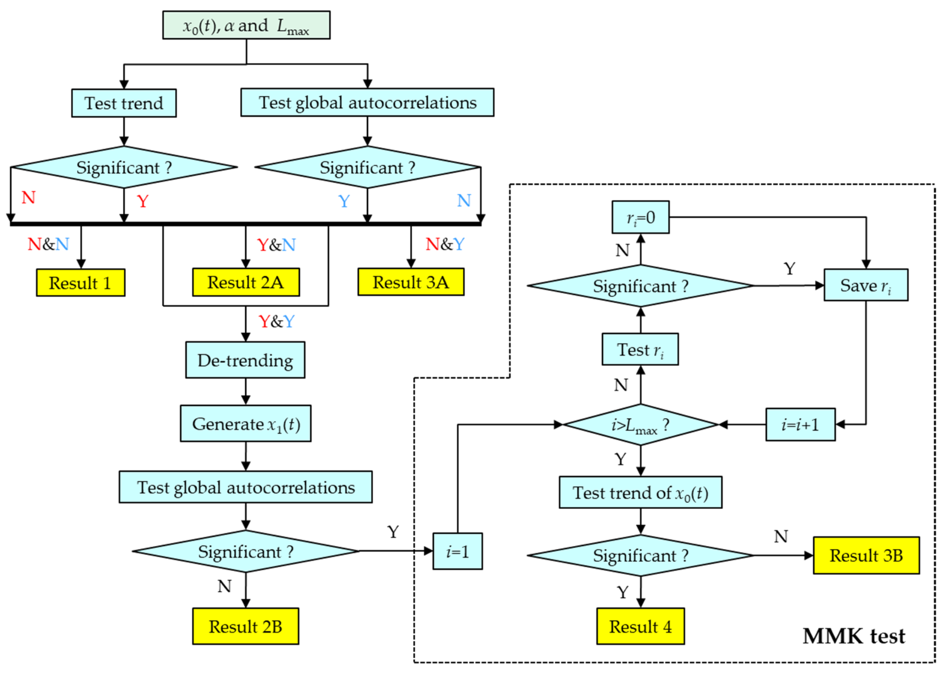
The flow chart of trend test based on the MMK test is shown in Figure 3. As can be seen from Figure 3, there are six detailed results (Results 1, 2A, 2B, 3A, 3B, and 4) corresponding to the six detailed interaction scenarios (Scenarios 1, 2A, 2B, 3A, 3B, and 4) in Figure 1. The MMK test is employed to distinguish Scenarios 3B and 4 in the trend test. For an original time series x₀(t) (t = 1, …, n), the trend test steps based on the MMK test are shown as follows:

• Step 1 Input x₀(t), and preset the significance level (α) and the maximum lag (L_max = floor(n/4), where floor denotes the floor function) of autocorrelation coefficient in the order-by-order test;
• Step 2 Test the trend in x₀(t) using Equations (1) and (2), and simultaneously test the global autocorrelations of x₀(t) by Equations (5)~(8);
• Step 3 Output Result 1 if neither the trend nor the global autocorrelations are significant, output Result 2A if the trend is significant and the global autocorrelations are not significant, output Result 3A if the global autocorrelations are significant and the trend is not significant, and then terminate the trend test;
• Step 4 Conduct the de-trending operation for x₀(t) using Equations (9)~(11), thus, generating the de-trended time series x₁(t) if the trend and autocorrelations are significant;
• Step 5 Test the global autocorrelations of x₁(t), output Result 2B if the global autocorrelations are not significant, and then terminate the trend test;
• Step 6 Test the autocorrelation coefficient r_i (i = 1, …, L_max) order by order if the global autocorrelations are significant, and then test the trend of x₀(t) by Equations (3) and (4);
• Step 7 Output Result 3B if the trend is not significant; otherwise, output Result 4 and terminate the trend test.

2.2.2. Trend Test Based on the OW Operation

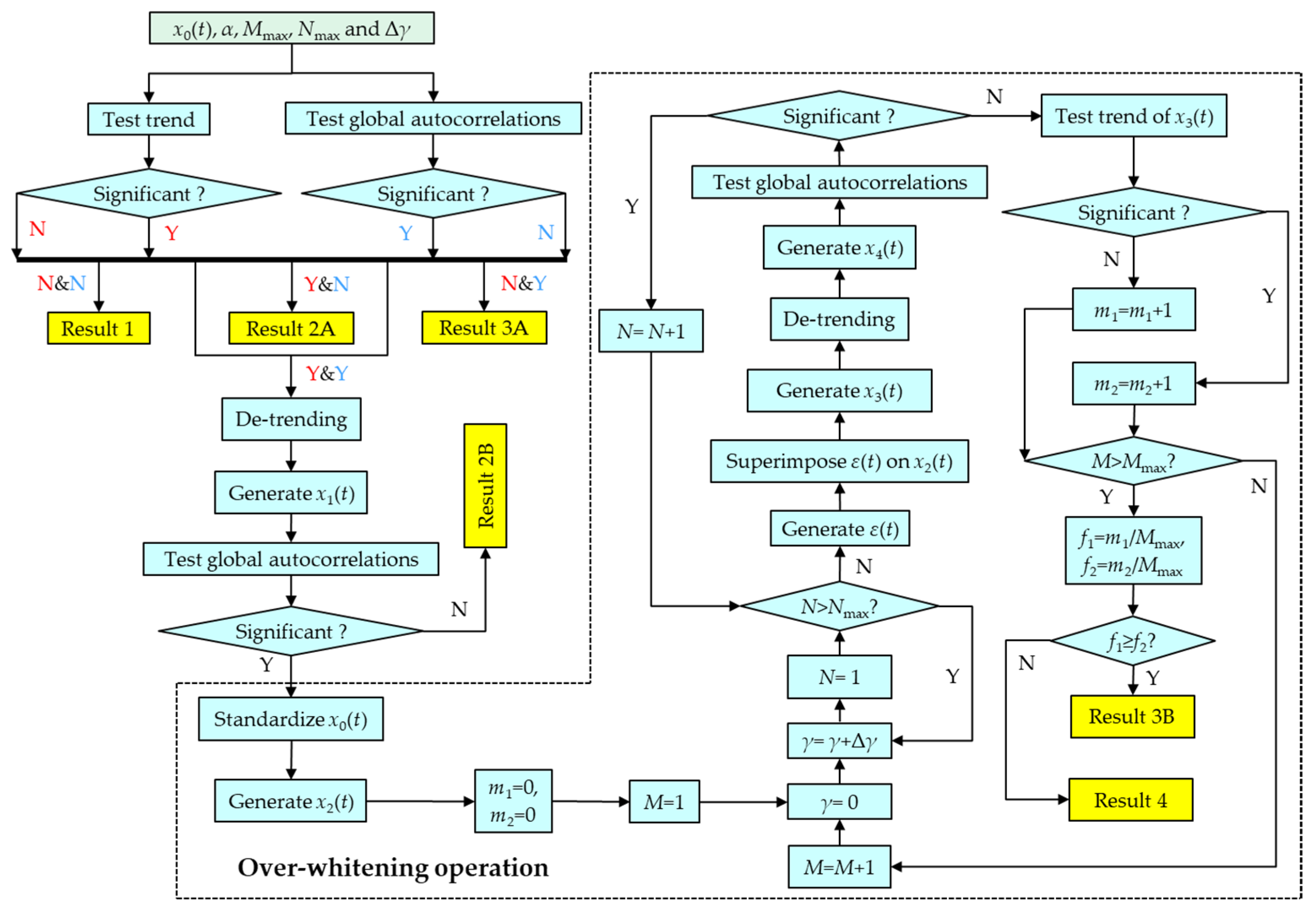
The trend test process based on the OW operation is displayed in Figure 4. From Figure 4, it can be seen that the OW operation is applied to discriminate Scenarios 3B and 4 in the trend test. Trend test steps based on the OW operation are given as below:

• Step 1 Input x₀(t), α, the maximum number (M_max = 1000) of simulations, the maximum number (N_max = 10) of cycles for OW operation, and the increasing step (Δγ = 0.1) of variance of the Gaussian white noise;
• Steps 2~5 can be referred to the same steps in the trend test based on the MMK test;
• Step 6 Standardize x₀(t) to generate the standardized time series x₂(t) by Equation (12);
• Step 7 Generate a Gaussian white noise ε(t) with the variance of γ, and superimpose ε(t) on x₂(t), thus, generating x₃(t);
• Step 8 Conduct the de-trending operation for x₃(t) using Equations (9)~(11), and thus, generating x₄(t);
• Step 9 Test the global autocorrelations of x₄(t), and then return to Step 7 if the global autocorrelations are significant and the current number (N) of cycles for the OW operation does not reach N_max;
• Step 10 Increase γ in steps of Δγ, and then return to Step 7 if N is larger than N_max and the global autocorrelations are still significant;
• Step 11 Test the trend of x₃(t) if the global autocorrelations are not significant, and then record the current number (M) of simulations;
• Step 12 Accumulate for the number m₁ if the trend is not significant; otherwise, accumulate for the number m₂;
• Step 13 Return to Step 10 if M is not larger than M_max; otherwise, calculate the percentages (f₁ and f₂) of m₁ and m₂ in M;
• Step 14 Output Result 3B if f₁ is not smaller than f₂; otherwise, output Result 4, and then terminate the trend test.

As can be seen from Figure 4, an outer loop is designed to calculate the occurrence frequencies (f₁ and f₂) of significant and non-significant trends in the OW operation. The designed outer loop is the strategy of this study to ensure the reliable trend test results using the OW operation. Based on f₁ and f₂, it is clear whether an HCTS has a significant trend or a significant pseudo trend.

2.3. Simulation Experiments

2.3.1. Generation of Sample Time Series

The autoregressive moving average model ARMA (1, 1) is often used to generate STS to verify the performance of a trend test method [7,11]. The first number 1 and the second number 1 represent the autoregressive order and the moving average order, respectively. In this study, the ARMA (1, 1) model with a built-in linear trend is established to generate sample time series (STS), i.e., x(t), which is formulated as:

$$x\left(t\right)=\varphi \cdot x\left(t-1\right)+\xi \left(t\right)+\theta \cdot \xi \left(t-1\right)+k\cdot t$$

(15)

where ϕ (0 < ϕ < 1) and θ (0 < θ < 1) represent the autoregressive coefficient and moving average coefficient, respectively; k (0 < k < 0.1) denotes the trend slope; and ξ(t) is the random error series following the standard normal distribution.

2.3.2. Introduction to Simulation Experiments

This study designs two simulation experiments to assess the performance of trend tests based on the MMK test and OW operation, and the influence of significance level on the trend test is analyzed. In each simulation experiment, 1000 STSs are generated by Equation (15) randomly. Note that the moving average coefficient θ in both experiments is equal to zero to simplify the simulations.

(1)

Simulation experiment 1

The 1000 STSs are randomly generated by

$$x\left(t\right)=\{\begin{array}{l}\xi \left(t\right), \mathrm{if} 0\le R{N}_1\le 0.25 ;\\ \xi \left(t\right)+\left(0.02+0.04R{N}_2\right)\cdot t, \mathrm{if} 0.25<R{N}_1\le 0.5 ;\\ \left(0.3+0.4R{N}_3\right)\cdot x\left(t-1\right)+\xi \left(t\right), \mathrm{if} 0.5<R{N}_1\le 0.75 ;\\ \left(0.3+0.4R{N}_3\right)\cdot x\left(t-1\right)+\xi \left(t\right)+\left(0.02+0.04R{N}_2\right)\cdot t, \mathrm{if} 0.75<R{N}_1\le 1 .\end{array}$$

(16)

where RN₁, RN₂, and RN₃ are three uniform random numbers, 0 ≤ RN₁, RN₂, RN₃ ≤ 1.

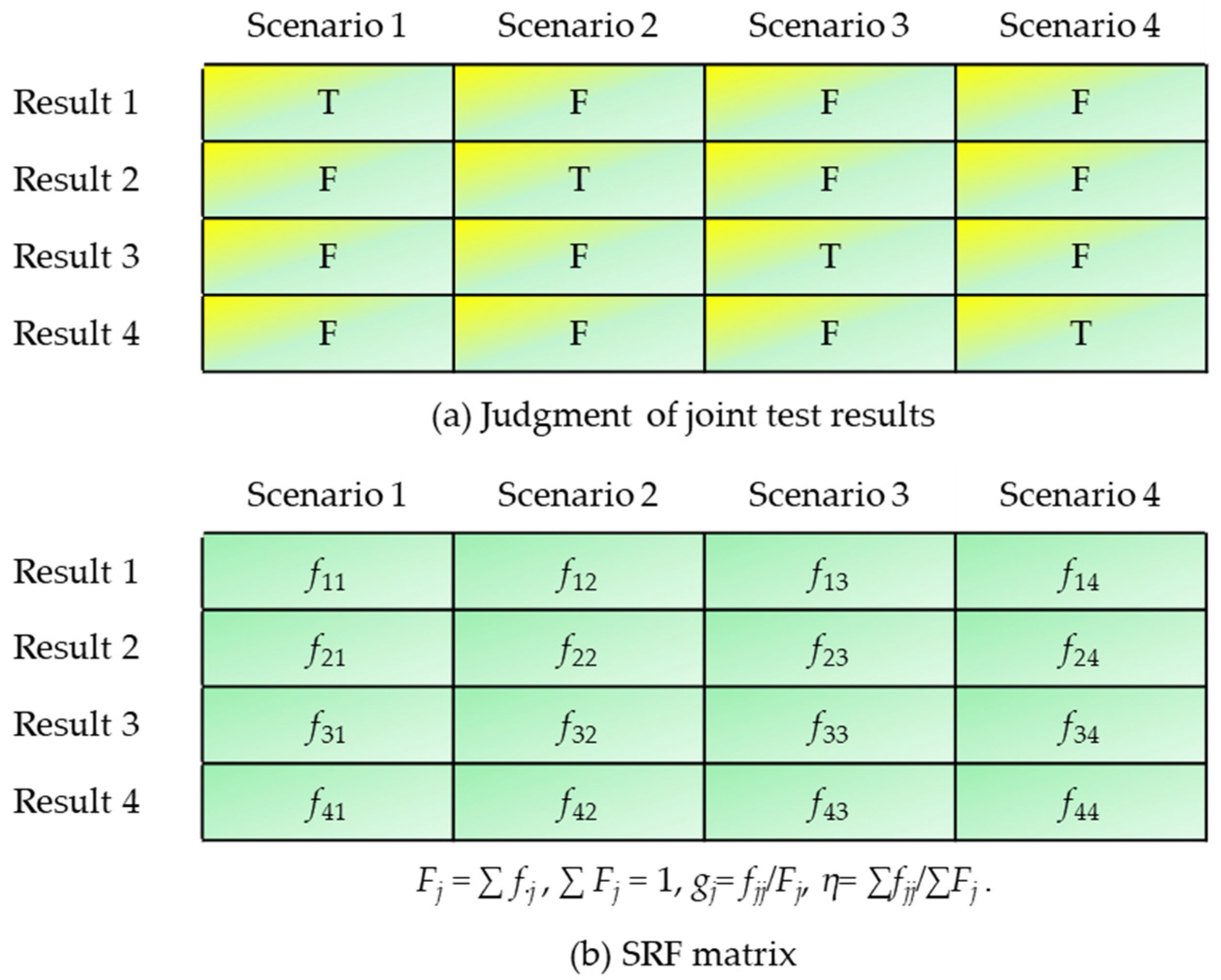
Under the same significance level, the trend of each STS is tested by the MMK test and OW operation, respectively. As shown in Figure 5a, the trend test result is true if Result i (i = 1, …, 4) corresponds to Scenario i, otherwise, the test result is false. Note that Result 2 includes Results 2A and 2B, and Result 3 contains Results 3A and 3B.

The effect of significance level on trend tests can be determined according to the trend test results. Meanwhile, the performance of each trend test method also can be evaluated.

(2)

Simulation experiment 2

Another 1000 STSs are generated by

$$x\left(t\right)=\{\begin{array}{l}\xi \left(t\right), if 0\le RN\le 0.25;\\ \xi \left(t\right)+k\cdot t, if 0.25<RN\le 0.5;\\ \varphi \cdot x\left(t-1\right)+\xi \left(t\right), if 0.5<RN\le 0.75 ;\\ \varphi \cdot x\left(t-1\right)+\xi \left(t\right)+k\cdot t, if 0.75<RN\le 1 .\end{array}$$

(17)

where RN denotes a uniform random number; ϕ = 0.3, 0.5, and 0.7; and k = 0.02, 0.04, and 0.06.

Unlike simulation experiment 1, the main objective of simulation experiment 2 is to examine the impacts of trend and autocorrelations on the performances of the MMK test and OW operation. As can be seen from Figure 5b, the scenario–result frequency (SRF) matrix is composed of the occurrence frequency (f_ij) of Result i (i = 1, …, 4) corresponding to Scenario j (j = 1, …, 4). Based on the SRF matrix, the accuracy rate (g_j) for Scenario j and the overall accuracy rate (η) can be applied to evaluate the effectiveness of these two trend test methods.

3. Application to STS

3.1. Preliminary Verification for Two Trend Test Methods

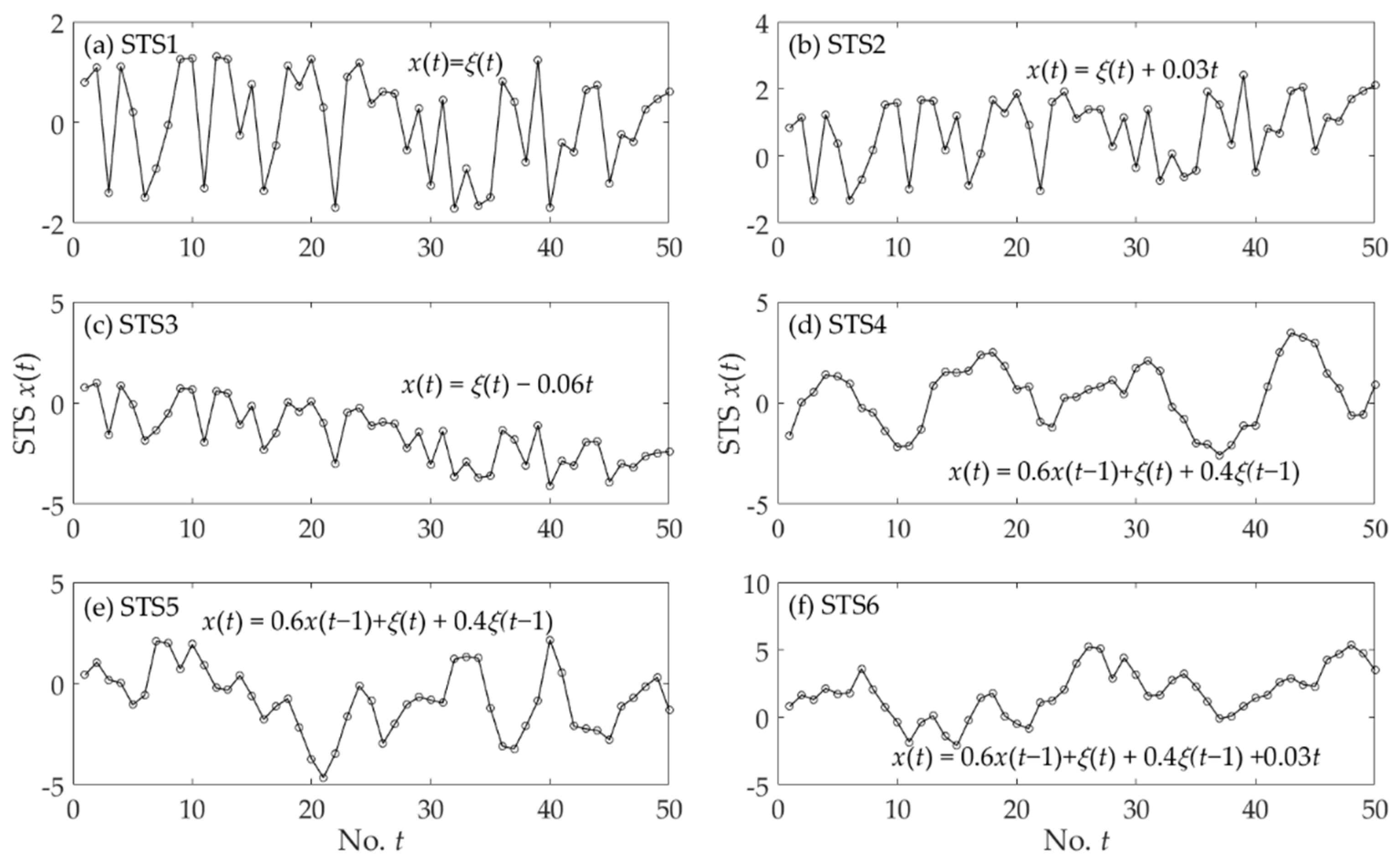
As shown in Figure 6, six STSs (STS1, …, STS6) with a length of 50 are generated based on Equation (15). The interaction scenarios of STS1, STS2, STS3, STS4, STS5, and STS6 correspond to Scenarios 1, 2, 3, 4, 5, and 6, respectively. Particularly, STS4 and STS5 are generated from the same model: x(t) = 0.6x(t − 1) + ξ(t) + 0.4ξ(t − 1), t = 1, …, 50.

The trend tests based on the MMK test and OW operation are applied to the six STSs, and the results are shown in

Table 1. Trend test results of the six STSs based on the MMK test and OW operation at 5% significance level.

STS	STS1	STS2	STS3	STS4	STS5	STS6
Result I	1	2A	2B	3A	3B	4
Result II	1	2A	2B	3A	3B	4
kI	0	0.019	−0.071	0	0	0.060
kII	0	0.019	−0.071	0	0	0.059
γa	0	0	0	0	0.66	0.75
f1 (%)	0	0	0	0	66.0	13.2
f2 (%)	0	0	0	0	34.0	86.8

Note: Results I and II represent results of the MMK test and OW operation, respectively; k_I and k_II denote the trend slopes of STS derived by the MMK test and OW operation, respectively; γ_a is the average minimum variance of white noise in the trend test based on the OW operation; and f₁ and f₂ are the occurrence frequencies of Results 3B and 4 in the trend test based on the OW operation, respectively.

. It demonstrates that results of the MMK test and OW operation are consistent for the same STS. Moreover, the trend test results for STS1 to STS6 correspond well to scenarios 1, 2A, 2B, 3A, 3B, and 4, respectively. Based on the two trend test methods, the calculated trend slopes (0.019 and −0.071) for STS2 and STS3 are close to their true ones (0.03 and −0.06), but the calculated trend slopes (k_I = 0.060 and k_II = 0.059) of STS6 deviate significantly from its true one (0.03). In the trend tests based on the OW operation, the average minimum variances (γ_a) of superimposed white noise are 0.66 and 0.75 for STS5 and STS6, respectively. Moreover, the occurrence frequencies (f₁ and f₂) of Results 3B and 4 are 66% and 34% for STS5 and 13.2% and 86.8% for STS6.

3.2. Results of Simulation Experiment 1

Table 2. Accuracy rates of trend tests in simulation experiment 1 at different significance levels. Unit: %.

N	MMK Test			OW Operation
	α = 10%	α = 5%	α = 1%	α = 10%	α = 5%	α = 1%
30	58.7	57.8	48.2	59.3	59.4	51.4
50	76.3	81.9	78.8	76.7	80.8	78.0
100	83.0	88.8	95.3	81.1	87.7	93.0

Note: N is the length of STS; and α denotes the significance level.

shows the accuracy rates of trend tests based on the MMK test and OW operation at different significance levels. One can see that the accuracy rates of the two methods increased significantly with the increasing length (n) of STS at the same significance level (α). For the STS of length 30, the accuracy rate of MMK test decreased as α decreased, and the accuracy rate of the OW operation at the 1% significance level was less than that at the 5% (10%) significance level. With respect to the STS of length 50, the accuracy rates of the two methods initially increased and then decreased as α decreased. When the length of STS increased to 100, the accuracy rates of the two methods increased as α decreased. Overall, the accuracy rates of the two methods were always lower than 1 − α at the significance level α, and the accuracy rates gradually approached 1 − α with a decrease in α when the length of the STS was long enough. In particular, for the STS of length 100, the accuracy rates of the two methods were less than 90%, 95%, and 99% at the 10%, 5%, and 1% significance levels, respectively; and the differences between the accuracy rate of the MK test (OW operation) and 1 − α were 7.0% (8.9%), 6.2% (7.3%), and 3.7% (6.0%) at the 10%, 5%, and 1% significance levels, respectively.

It can also be seen from Table 2 that the accuracy difference between the MMK test and OW operation was always not more than 3.5% for the STS of the same length at the same significance level. In addition, for the STS of length 30, the accuracy rate of the OW operation was larger than that of the MMK test at the same significance level. For the STS of length 50, the accuracy rate of the MMK test was slightly less than that of the OW operation at the 10% significance level, but the opposite was true at the 5% and 1% significance levels. When the length of the STS increased to 100, the accuracy rate of the MMK test was larger than that of the OW operation at the same significance level.

The results of the trend tests based on the MMK test and OW operation are shown in

Table 3. Judgement for trend test results in simulation experiment 1 at the 5% significance level. Unit: %.

N	f(TI&TII)	f(TI&FII)	f(FI&TII)	f(FI&FII)	f(TI)	f(TII)	f(TI&TII or FI&FII)	ra
30	56.6	1.2	2.8	39.4	57.8	59.4	96.0	59.0
50	79.9	2.0	0.9	17.2	81.9	80.8	97.1	82.3
100	87.6	1.2	0.1	11.1	88.8	87.7	98.7	88.8

Note: T_I and T_II represent when the trend test results of MMK test and OW operation are truthful; F_I and F_II denote when the trend test results of MMK test and OW operation are false; f () represent the occurrence frequency of a result; and r_a is the accurate rate of the MMK test and OW operation when their trend test results are consistent, and r_a = f(T_I&T_II)/f(T_I&T_II or F_I&F_II) × 100%.

. It shows that the possibility of correct tests of both methods increased, while the possibility of false tests for both methods decreased as the length of STS increased. Moreover, the likelihood of consistent test results between the two methods exceeded 95% under the 5% significance level, and it also increased as the length of STS increased. When the test results of the two methods were consistent, the accuracy rate of the test result improved with the increasing length of STS. Particularly, the accuracy rate of the joint test of the two methods was more than 80% when the length of STS was not less than 50. In addition, there were cases where the trend test result of the MMK test (OW operation) was correct while that of the OW operation (MMK test) was incorrect, but the frequencies of such cases did not exceed 3%.

3.3. Results of Simulation Experiment 2

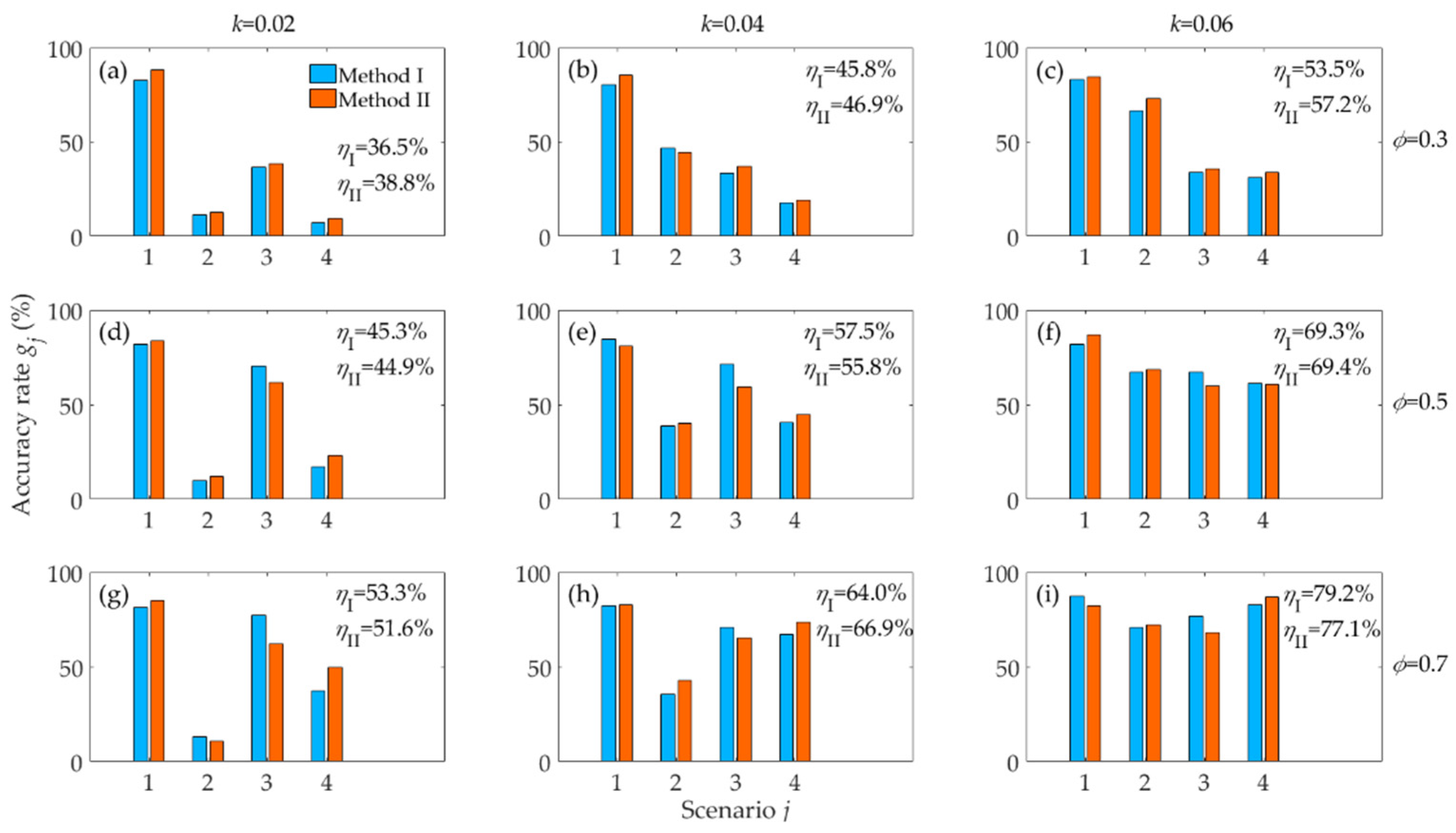
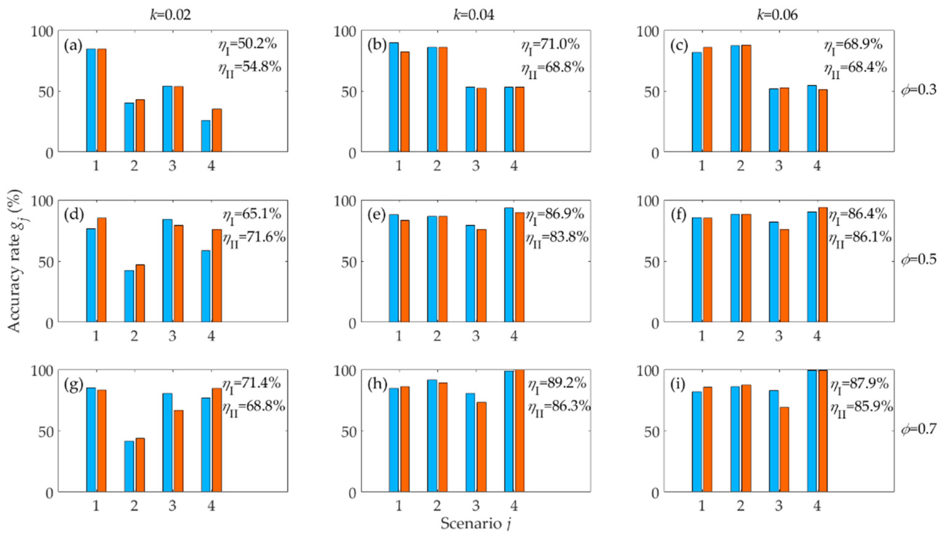
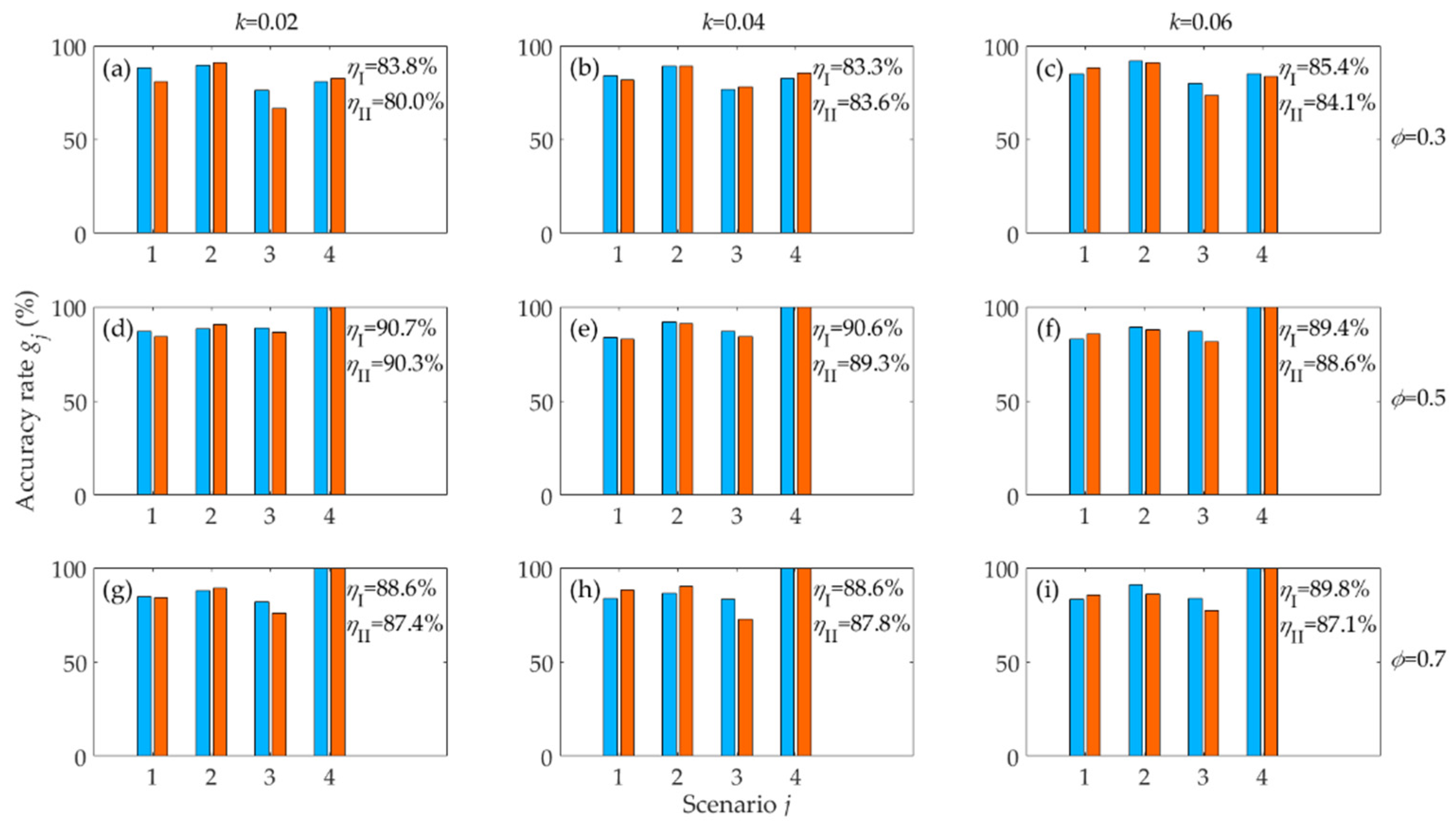
The SRF matrixes derived by the trend tests based on the MMK test and OW operation under the 5% significance level can be seen in

Table A1. SRF matrixes derived by the MMK test in simulation experiment 2 at the 5% significance level. Unit: %.

n	ϕ	k = 0.02				k = 0.04				k = 0.06
30	0.3	23.9	20.2	10.8	9.2	22.1	10.7	12.5	4.7	20.7	5.9	13.9	0.8
		1.4	2.7	2.7	4.1	2.1	11.2	3.4	9.8	1.1	16.1	2.6	14.1
		3.6	1.3	8.1	9.5	3.3	1.8	8.3	4.9	3.1	0.5	8.9	2.2
		0.0	0.1	0.6	1.8	0.0	0.2	0.8	4.2	0.0	1.6	0.7	7.8
	0.5	20.3	17.7	3.9	3.3	18.4	14.6	3.6	0.8	20.6	5.9	3.7	0.2
		1.0	2.3	2.2	5.0	0.8	10.7	2.0	6.8	0.9	16.6	2.5	7.1
		3.4	2.9	18.1	13.7	2.5	1.6	18.1	7.4	3.5	1.2	16.1	2.9
		0.1	0.0	1.5	4.6	0.0	0.8	1.6	10.3	0.1	1.0	1.7	16.0
	0.7	20.9	18.5	1.0	0.2	21.5	13.7	1.0	0.1	19.8	5.1	1.1	0.1
		1.4	3.3	1.0	0.8	1.1	9.1	1.3	1.9	1.2	17.4	1.0	2.3
		3.2	3.1	20.5	13.4	3.5	1.6	16.9	6.0	1.6	0.7	21.6	1.9
		0.1	0.0	4.0	8.6	0.0	1.2	4.6	16.5	0.0	1.4	4.4	20.4
50	0.3	19.4	12.5	9.7	3.5	23.5	1.2	10.0	0.0	20.6	0.0	10.2	0.0
		0.7	9.8	1.8	9.0	1.0	21.5	1.6	9.8	1.8	21.9	1.6	10.6
		2.8	1.5	14.0	7.4	1.6	0.0	14.0	0.7	2.7	0.0	13.6	0.0
		0.0	0.5	0.4	7.0	0.1	2.3	0.7	12.0	0.1	3.2	0.9	12.8
	0.5	17.3	12.1	1.1	0.3	20.0	0.6	1.6	0.0	19.7	0.0	1.1	0.0
		1.1	10.9	0.3	1.7	0.9	22.5	0.6	1.6	0.9	22.2	0.7	2.3
		4.2	2.0	22.1	8.6	1.9	0.2	19.1	0.2	2.3	0.0	23.0	0.0
		0.0	0.7	2.8	14.8	0.0	2.7	2.8	25.3	0.1	2.9	3.3	21.5
	0.7	20.9	11.5	0.0	0.0	20.5	0.7	0.2	0.0	18.6	0.0	0.0	0.0
		1.5	10.1	0.1	0.0	1.1	26.4	0.0	0.2	1.8	20.8	0.2	0.2
		2.1	1.6	22.4	5.4	2.6	0.3	18.0	0.1	2.3	0.0	21.2	0.0
		0.0	1.0	5.4	18.0	0.0	1.5	4.1	24.3	0.0	3.4	4.2	27.3
100	0.3	21.9	0.0	2.8	0.0	20.8	0.0	3.1	0.0	19.3	0.0	2.5	0.0
		0.8	22.3	1.0	4.9	1.3	22.4	0.9	4.5	1.1	22.5	0.6	4.0
		2.1	0.0	18.7	0.0	2.6	0.0	18.6	0.0	2.3	0.0	20.8	0.0
		0.0	2.6	2.0	20.9	0.0	2.7	1.6	21.5	0.0	2.0	2.1	22.8
	0.5	22.8	0.0	0.0	0.0	21.2	0.0	0.0	0.0	21.8	0.0	0.0	0.0
		1.0	23.0	0.0	0.1	1.5	23.1	0.0	0.1	1.7	21.9	0.0	0.0
		2.5	0.0	20.3	0.0	2.6	0.0	21.6	0.0	2.8	0.0	22.4	0.0
		0.0	3.1	2.6	24.6	0.0	2.0	3.2	24.7	0.0	2.7	3.4	23.3
	0.7	19.6	0.0	0.0	0.0	21.8	0.0	0.0	0.0	20.4	0.0	0.0	0.0
		1.0	23.6	0.0	0.0	1.7	19.8	0.0	0.0	1.5	24.2	0.0	0.0
		2.6	0.0	20.7	0.0	2.5	0.0	20.6	0.0	2.6	0.0	18.9	0.0
		0.0	3.3	4.5	24.7	0.0	3.1	4.1	26.4	0.0	2.4	3.7	26.3

Note: n is the length of STS; and ϕ and k separately denote the autoregressive coefficient and the trend slope preset in simulation experiment 2.

and

Table A2. SRF matrixes derived by the OW operation in simulation experiment 2 at the 5% significance level. Unit: %.

n	ϕ	k = 0.02				k = 0.04				k = 0.06
30	0.3	25.0	18.1	11.0	10.7	22.0	12.3	12.3	4.2	20.7	5.4	11.8	1.5
		1.0	3.0	1.8	3.9	1.5	11.3	1.7	11.3	1.0	19.7	2.4	13.5
		2.3	2.4	8.3	9.2	2.2	1.3	8.8	5.0	2.8	0.7	8.3	1.7
		0.0	0.3	0.5	2.5	0.1	0.4	0.8	4.8	0.0	1.1	0.9	8.5
	0.5	21.7	19.2	4.5	2.4	19.3	12.8	4.1	1.3	22.9	6.3	4.2	0.1
		1.3	3.1	1.9	3.9	0.9	10.5	2.7	6.7	1.3	17.9	2.4	7.6
		3.0	3.4	14.3	12.9	3.6	2.2	14.5	6.2	2.2	0.7	15.5	0.8
		0.0	0.2	2.4	5.8	0.0	0.6	3.1	11.5	0.0	1.2	3.8	13.1
	0.7	20.9	19.6	0.7	0.2	21.4	11.0	0.7	0.1	20.3	4.9	0.9	0.0
		1.1	2.8	1.6	2.1	0.7	9.9	1.3	3.5	0.9	17.6	1.5	2.4
		2.6	3.0	15.4	10.3	3.7	1.5	16.4	3.2	3.4	0.2	18.4	0.7
		0.0	0.1	7.1	12.5	0.0	0.7	6.7	19.2	0.1	1.7	6.2	20.8
50	0.3	22.1	12.4	8.3	2.4	20.7	1.0	8.3	0.0	20.7	0.0	9.9	0.0
		1.1	11.1	1.8	7.9	1.6	22.1	2.0	11.7	1.0	20.2	1.2	12.9
		2.8	1.2	13.6	4.5	2.9	0.1	12.6	0.0	2.4	0.0	13.9	0.0
		0.1	1.0	1.7	8.0	0.0	2.5	1.1	13.4	0.0	2.8	1.4	13.6
	0.5	20.3	11.2	1.1	0.3	22.3	0.9	1.2	0.0	21.4	0.0	0.8	0.0
		1.2	12.1	0.8	1.7	1.5	21.8	0.9	2.4	1.3	22.4	0.7	1.6
		2.3	1.8	22.1	3.4	2.9	0.0	18.7	0.0	2.4	0.0	17.7	0.0
		0.0	0.7	3.9	17.1	0.1	2.5	3.8	21.0	0.0	3.0	4.1	24.6
	0.7	20.9	13.3	0.0	0.0	22.0	0.6	0.0	0.0	22.4	0.0	0.0	0.0
		1.6	11.5	0.0	0.3	1.3	21.6	0.2	0.1	1.5	21.1	0.0	0.2
		2.6	1.0	17.2	3.2	2.3	0.0	20.0	0.0	2.3	0.0	15.5	0.0
		0.0	0.6	8.6	19.2	0.0	2.0	7.2	22.7	0.0	3.1	7.0	26.9
100	0.3	19.9	0.0	4.0	0.0	18.6	0.0	3.3	0.0	22.3	0.0	2.9	0.0
		1.6	21.8	1.5	4.2	1.6	21.9	0.7	3.9	0.9	22.6	0.8	4.0
		3.0	0.0	18.0	0.0	2.6	0.0	20.4	0.0	2.1	0.0	18.5	0.0
		0.1	2.1	3.5	20.3	0.0	2.6	1.7	22.7	0.0	2.3	2.9	20.7
	0.5	23.0	0.0	0.0	0.0	20.2	0.0	0.0	0.0	21.6	0.0	0.0	0.0
		1.4	22.7	0.0	0.0	1.3	22.1	0.0	0.1	1.7	22.6	0.0	0.0
		2.9	0.0	19.7	0.0	2.9	0.0	22.1	0.0	1.9	0.0	20.4	0.0
		0.0	2.3	3.1	24.9	0.0	2.2	4.2	24.9	0.0	3.1	4.7	24.0
	0.7	19.4	0.0	0.0	0.0	21.8	0.0	0.0	0.0	20.2	0.0	0.0	0.0
		1.0	25.0	0.0	0.0	1.2	23.4	0.0	0.0	1.1	22.0	0.0	0.0
		2.6	0.0	18.5	0.0	1.7	0.0	18.1	0.0	2.3	0.0	20.3	0.0
		0.1	3.0	5.9	24.5	0.0	2.5	6.8	24.5	0.0	3.6	5.9	24.6

Note: the meanings of n, ϕ, and k can be found in Table A1.

in Appendix A. According to the SRF matrixes, the accuracy rates of two trend test methods for the STSs of lengths 30, 50, and 100 are shown in Figure 7, Figure 8 and Figure 9, respectively.

From Figure 7, Figure 8 and Figure 9, it can be seen that the accuracy rate (g₁) of the trend test based on the MMK test (former accuracy rate) was between 76.5% and 89.7% for Scenario 1, and that of the trend test based on the OW operation (latter accuracy rate) ranged from 80.9% to 88.3%. For Scenario 2 (2A and 2B), the former and latter accuracy rates (g₂) were 10.0~92.0% and 11.0~91.2%, respectively. With respect to Scenario 3 (3A and 3B), the former and latter accuracy rates (g₃) are 33.2~88.6% and 35.5~86.4%, respectively. With regard to Scenario 4, the former and latter accuracy rates (g₄) varied from 7.3% to 100% and 9.5% to 100%, respectively. In addition, the accuracy rates (g₂, g₃ ang g₄) of trend tests basically increased with the increasing values of k and ϕ, as well as with the increasing length of the STS.

In Figure 7, when the length of STS was 30, the overall accuracy rate of the trend tests based on the MMK test (η_I) and OW operation (η_II) increased with the growth of trend slope (k) and autoregressive coefficient (ϕ). When the length of STS was 50, Figure 8 shows that the value of η_I initially increased and then decreased as the value of k increased, and the change of η_II also followed this pattern roughly. Additionally, the value of η_I increased with the increase in ϕ value. When the value of ϕ increased from 0.3 to 0.5, the value of η_II increased immediately, but when the value of ϕ increased from 0.5 to 0.7, it decreased slightly or increased slowly. As can be found in Figure 9, the values of η_I and η_II for the STS of length 100 for the STS of length 100 always exceeded 80%. However, the variations of η_I and η_II for the STS of length 100 were not as significant and regular as those for the STSs of lengths 30 and 50 with increasing values of k and ϕ. Additionally, Figure 7, Figure 8 and Figure 9 together show that the values of η_I and η_II were similar. In general, η_I was slightly less than η_II when the length (n) of STS was short and the autocorrelations (ϕ) of STS were weak; otherwise, η_I was basically more than η_II. Specifically, for the STS of length 30 (Figure 7), η_II was 1.1~3.7% more than η_I when ϕ equaled 0.3, and η_I was close to or even exceeded η_II when ϕ was 0.5. When n increased to 100 (Figure 9), η_I was 0.4~3.8% more than η_II, except for the case where ϕ was 0.3 and k equaled 0.4 (η_I = 83.3% and η_II = 83.6%).

4. Application to HCTS

4.1. Study Area and Data

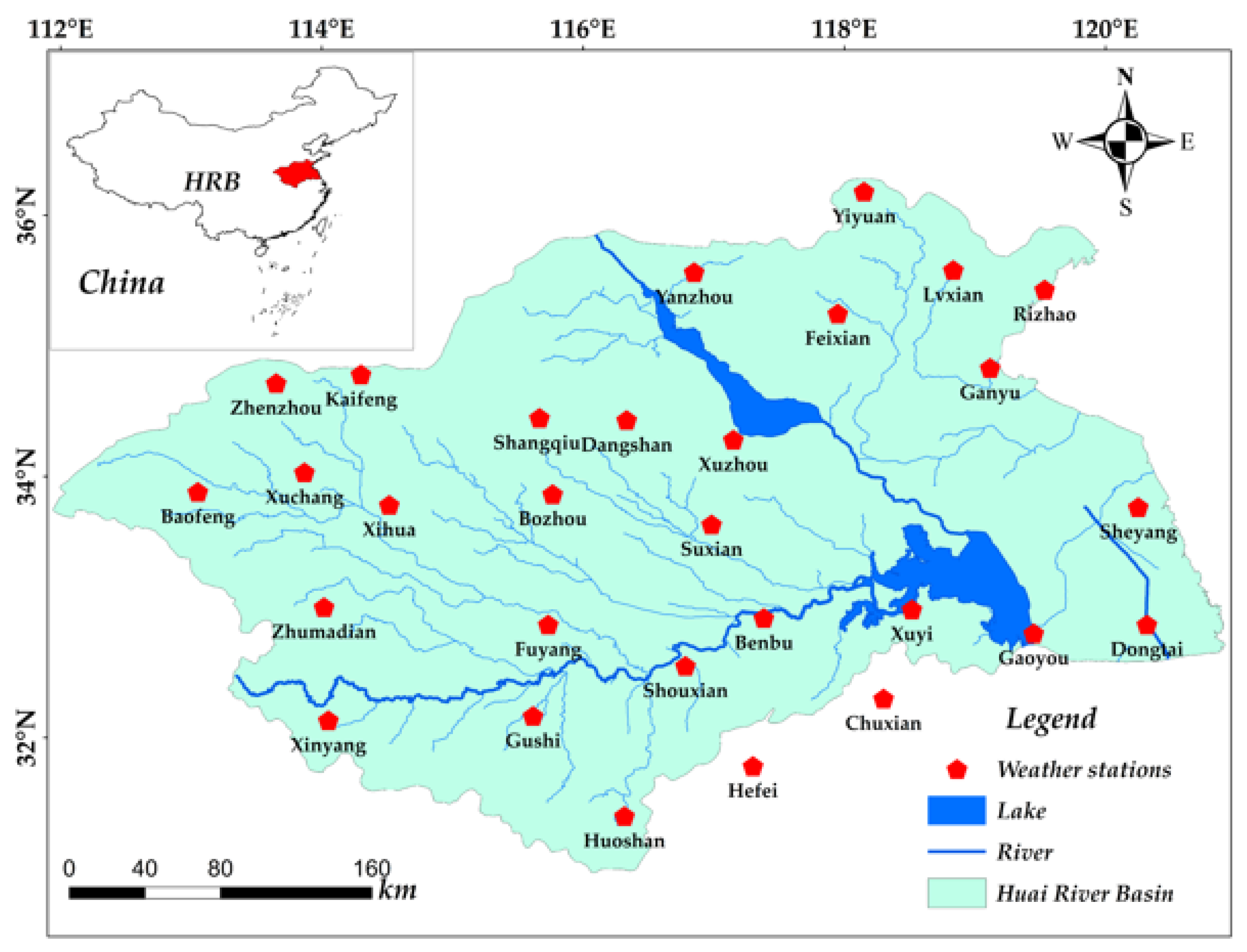
The Huaihe River Basin (HRB) is a significant transition zone for geographic elements in eastern China and a sensitive area for climate change [24]. Additionally, the HRB is also an important grain production base in China with a watershed area of 270,000 km².

In the study, the annual precipitation (P), sunshine duration (SD), average temperature (AT), wind speed (WS), relative humidity (RH), and potential evapotranspiration (PET) series (1960~2020, 61 years in total) at the 29 national weather stations in or around the HRB (Figure 10) were employed to verify the performances of trend tests based on the MMK test and OW operation. Among the six HCTSs, the P, SD, AT, WS, and RH data can be downloaded from the website: http://data.cma.cn/. The PET data were calculated by the Penman–Monteith formula [30], whose calculation software (EToCalculator) can be downloaded at the website: http://www.fao.org/land-water/databases-and-software/eto-calculator/en/ (accessed on 21 July 2022). In addition, there are no missing values in the six HCTSs and the data are highly quality controlled.

4.2. Trend Test Results of Six HCTSs

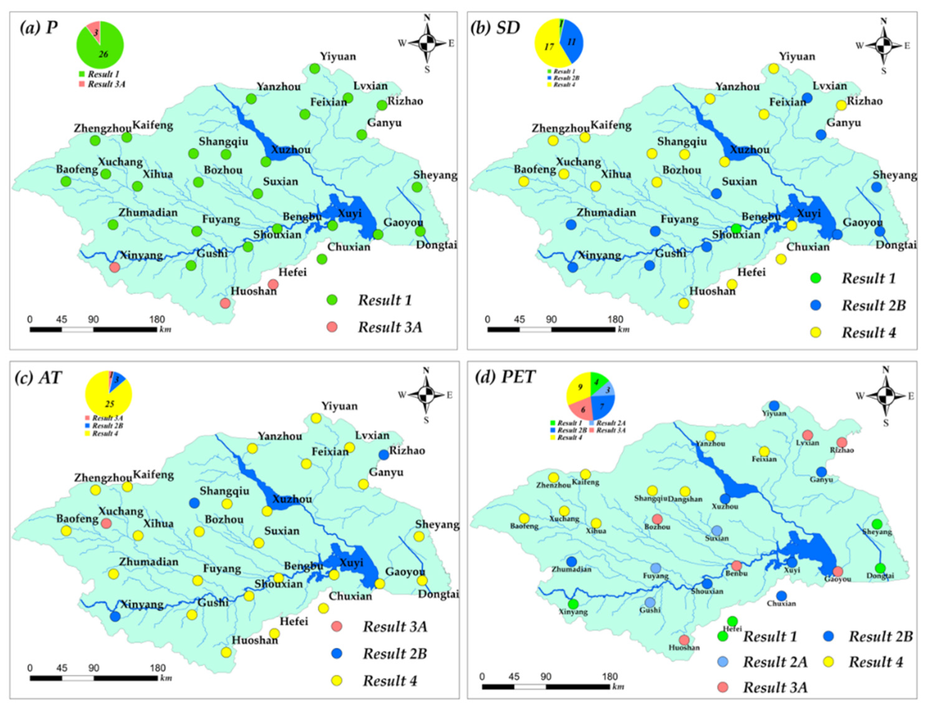
The trend test results for the six HCTSs in the HRB under the 5% significance level are shown in Figure 11 and Figure 12. It can be seen that all six detailed scenarios were present in the trend tests of HCTSs in HRB.

As shown in Figure 11, the results of the trend test based on the MMK test and OW operation are identical for the annual P, SH, AT, and PET series at each station in the HRB. Specifically, it can be seen from Figure 11a that there was neither a significant trend nor significant autocorrelations in the annual P series for 89.7% of the stations in the HRB, and there were only significant autocorrelations in the annual P series for other stations (Huoshan, Hefei, and Xinyang). Figure 11b shows that the annual SD series had neither a significant trend nor significant autocorrelations only at Bengbu station. Additionally, there were significant trends and significant autocorrelations in the annual SD series for 58.6% of the stations, and the annual SD series had only a significant trend for 37.9% of stations. In Figure 11c, the annual AT series had significant autocorrelations only at Xuchang station, while there were significant autocorrelations at three stations (Xinyang, Dangshan, and Rizhao). Additionally, there were significant trends and significant autocorrelations in the annual AT series for 86.2% of the stations. For the annual PET series in Figure 11d, 31.0% of the stations had both a significant trend and significant autocorrelations, 34.5% of the stations had only a significant trend, 20.7% of the stations had only significant autocorrelations, and 13.8% of the stations had neither a significant trend nor significant autocorrelations.

The trend slopes of annual SD, AT, and PET series derived from the MMK test and OW operation are shown in

Table 4. Trend slopes for the annual SD, AT, and PET series in the HRB derived by the trend tests based on the MMK test and OW operation at the 5% significance level.

No.	Station Name	SD (h/a)		AT (°C/a)		PET (mm/a)
		kI	kII	kI	kII	kI	kII
1	Huoshan	−0.02	−0.02	0.02	0.02	0.00	0.00
2	Hefei	−0.02	−0.03	0.02	0.02	0.00	0.00
3	Xinyang	−0.03	−0.03	0.03	0.03	0.00	0.00
4	Gushi	−0.02	−0.02	0.02	0.02	−1.07	−1.07
5	Chuxian	−0.03	−0.03	0.02	0.02	−2.14	−2.14
6	Shouxian	−0.02	−0.02	0.02	0.02	−1.39	−1.39
7	Gaoyou	−0.01	−0.01	0.04	0.04	0.00	0.00
8	Fuyang	−0.03	−0.03	0.02	0.02	−0.95	−0.95
9	Dongtai	−0.01	−0.01	0.03	0.03	0.00	0.00
10	Bengbu	0.00	0.00	0.02	0.02	0.00	0.00
11	Xuyi	−0.03	−0.02	0.02	0.02	−1.75	−1.75
12	Zhumadian	−0.03	−0.03	0.02	0.02	−1.94	−1.94
13	Suxian	−0.02	−0.02	0.03	0.03	−0.95	−0.95
14	Sheyang	−0.01	−0.01	0.03	0.03	0.00	0.00
15	Xihua	−0.03	−0.03	0.03	0.03	−3.38	−2.94
16	Bozhou	−0.03	−0.03	0.03	0.03	0.00	0.00
17	Baofeng	−0.03	−0.03	0.02	0.02	−3.00	−2.97
18	Xuchang	−0.03	−0.03	0.00	0.00	−1.84	−1.97
19	Xuzhou	−0.02	−0.01	0.03	0.03	−1.63	−1.63
20	Dangshan	−0.02	−0.02	0.02	0.02	−2.44	−2.38
21	Shangqiu	−0.04	−0.04	0.02	0.02	−3.50	−3.47
22	Zhengzhou	−0.03	−0.03	0.04	0.04	−2.35	−2.49
23	Kaifeng	−0.03	−0.03	0.04	0.04	−1.50	−1.48
24	Ganyu	−0.02	−0.02	0.03	0.03	−1.00	−1.00
25	Feixian	−0.03	−0.03	0.03	0.03	−2.58	−2.59
26	Rizhao	−0.02	−0.02	0.03	0.03	0.00	0.00
27	Yanzhou	−0.02	−0.02	0.02	0.02	−2.64	−2.61
28	Lvxian	−0.03	−0.03	0.03	0.03	0.00	0.00
29	Yiyuan	−0.03	−0.03	0.03	0.03	−1.45	−1.45

Note: Station No. ranks from low latitude to high latitude; and k_I and k_II are the trend slopes of HCTS derived by the trend tests based on the MMK test and OW operation, respectively.

. It can be found that all stations with significant trends in the annual SD series exhibited a downward trend, all stations with significant trends in the annual AT series showed an upward trend, and all stations with significant trends in the annual PET series had a downward trend. In addition, the trend slopes of annual SD (AT) series derived from the two methods were the same at all stations, but there were some differences in the trend slopes of PET at some stations. Particularly, the difference in trend slopes for the annual PET series reached 0.44 mm/a at Xihua station. Without considering the units of three HCTSs, the absolute value of the trend slope of the annual SD (AT) series at each station did not exceed 0.05/a, while the absolute values of the trend slope were not less than 1.00/a at the stations where there were significant trends in the annual PET series.

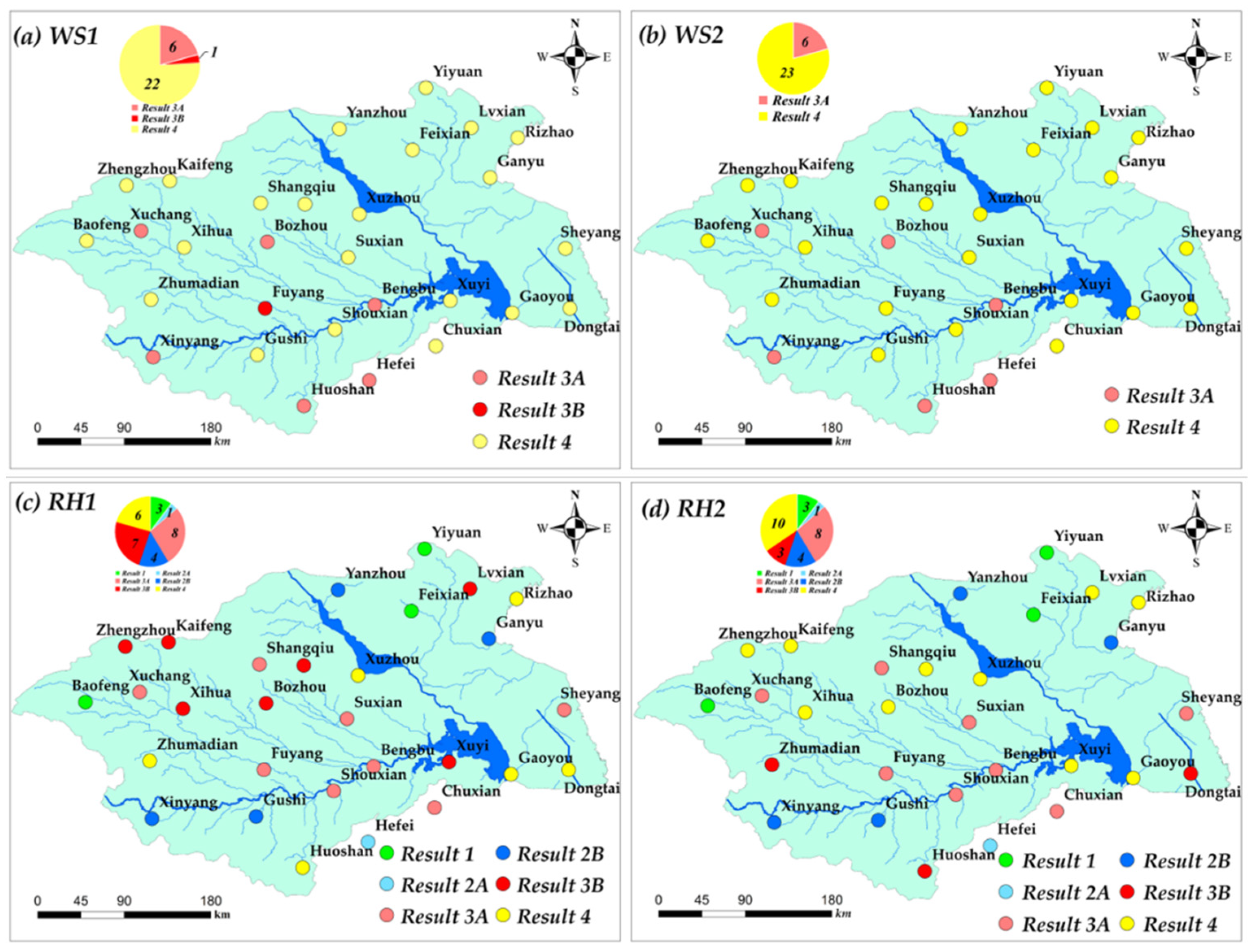
Figure 12 shows that for the annual series of WS and RH in the HRB, there were some differences in the trend test results based on these two methods. Specifically, for the annual WS series only at Fuyang station, the trend test result based on the MMK test was Result 3B, while the trend test result based on the OW operation was Result 4. Overall, there was a significant trend in the annual WS series for more than 75% of the stations. For the annual RH series, the trend test results based on the MMK test (OW operation) were Result 4 (Result 3B) at three stations (Huoshan, Dongtai, and Zhumadian), while the trend test based on the MMK test (OW operation) yielded Result 3B (Result 4) at seven other stations (Xuyi, Xihua, Bozhou, Shangqiu, Zhengzhou, Kaifeng, and Lvxian). As for the annual RH series, there was no significant trend for more than 50% of the stations.

The trend slopes and OW operation results for the annual WS and RH series are shown in

Table 5. Trend slopes and OW operation results for the annual WS and RH series in the HRB at the 5% significance level.

HCTS	Station No.	No. 1	No. 2	No. 3	No. 4	No. 5	No. 6	No. 7	No. 8	No. 9	No. 10	No. 11	No. 12	No. 13	No. 14	No. 15
WS	kI((m/s)/a)	0.00	0.00	0.00	−0.03	−0.02	−0.02	−0.02	0.00	−0.01	0.00	−0.03	−0.02	−0.01	−0.01	−0.03
	kII ((m/s)/a)	0.00	0.00	0.00	−0.03	−0.02	−0.02	−0.02	−0.01	−0.01	0.00	−0.03	−0.02	−0.01	−0.01	−0.03
	γa	0.00	0.00	0.00	0.30	0.36	0.50	0.33	0.86	0.75	0.00	0.12	0.50	0.35	0.49	0.35
	f1 (%)	0.0	0.0	0.0	0.0	0.0	0.0	0.0	7.8	0.7	0.0	0.0	0.0	0.0	0.0	0.0
	f2 (%)	0.0	0.0	0.0	100.0	100.0	100.0	100.0	92.2	99.3	0.0	100.0	100.0	100.0	100.0	100.0
	Station No.	No. 16	No. 17	No. 18	No. 19	No. 20	No. 21	No. 22	No. 23	No. 24	No. 25	No. 26	No. 27	No. 28	No. 29
	kI((m/s)/a)	0.00	−0.02	0.00	−0.03	−0.02	−0.02	−0.02	−0.02	−0.02	−0.02	−0.01	−0.02	−0.01	−0.01
	kII ((m/s)/a)	0.00	−0.02	0.00	−0.03	−0.02	−0.03	−0.02	−0.03	−0.02	−0.02	−0.02	−0.02	−0.01	−0.01
	γa	0.00	0.21	0.00	0.11	0.59	0.24	0.19	0.38	0.16	0.10	0.86	0.54	0.25	0.32
	f1 (%)	0.0	0.0	0.0	0.0	0.0	0.0	0.0	0.0	0.0	0.0	5.1	0.0	0.0	0.0
	f2 (%)	0.0	100.0	0.0	100.0	100.0	100.0	100.0	100.0	100.0	100.0	94.9	100.0	100.0	100.0
	Station No.	No. 1	No. 2	No. 3	No. 4	No. 5	No. 6	No. 7	No. 8	No. 9	No. 10	No. 11	No. 12	No. 13	No. 14	No. 15
RH	kI (%/a)	−0.03	−0.04	−0.10	−0.08	0.00	0.00	−0.16	0.00	−0.03	0.00	0.00	−0.05	0.00	0.00	0.00
	kII (%/a)	0.00	−0.04	−0.10	−0.08	0.00	0.00	−0.16	0.00	0.00	0.00	−0.05	0.00	0.00	0.00	−0.07
	γa	0.11	0.00	0.00	0.00	0.00	0.00	0.15	0.00	0.29	0.00	0.23	0.10	0.00	0.00	0.22
	f1 (%)	52.2	0.0	0.0	0.0	0.0	0.0	0.0	0.0	65.4	0.0	19.2	51.7	0.0	0.0	15.2
	f2 (%)	47.8	0.0	0.0	0.0	0.0	0.0	100.0	0.0	34.6	0.0	80.8	48.3	0.0	0.0	84.8
	Station No.	No. 16	No. 17	No. 18	No. 19	No. 20	No. 21	No. 22	No. 23	No. 24	No. 25	No. 26	No. 27	No. 28	No. 29
	kI (%/a)	0.00	0.00	0.00	−0.04	0.00	0.00	0.00	0.00	−0.04	0.00	−0.07	0.08	0.00	0.00
	kII (%/a)	−0.06	0.00	0.00	−0.04	0.06	0.00	−0.12	−0.15	−0.04	0.00	−0.07	0.08	−0.05	0.00
	γa	0.18	0.00	0.00	0.10	0.22	0.00	0.41	0.33	0.00	0.00	0.10	0.00	0.15	0.00
	f1 (%)	37.3	0.0	0.0	37.7	36.4	0.0	2.3	0.0	0.0	0.0	0.0	0.0	18.6	0.0
	f2 (%)	62.7	0.0	0.0	62.3	63.6	0.0	97.7	100.0	0.0	0.0	100.0	0.0	81.4	0.0

Note: Station No. ranks from low latitude to high latitude; k_I and k_II are the trend slopes of HCTS derived by the MMK test and OW operation, respectively; γ_a denotes the average minimum variance of white noise in the trend test of the OW operation; and f₁ and f₂ separately denote occurrence frequencies of Result 3B and 4 in the trend test of the OW operation.

. Most stations (MMK-22 stations and OW-23 stations) exhibited a significant downward trend in the annual WS series. Less than half of the stations (MMK-11 stations and OW-15 stations) showed a significant decreasing trend in the annual WS series, while only two stations (No. 20 Dangshan and No. 27 Yanzhou) displayed a significant increasing trend. Without considering the units, the trend slopes of two HCTSs were no more than 0.10/a. Additionally, when the trend test results were consistent, the two trend test methods could obtain the similar trend slope for the annual WS and RH series. From the average minimum variance of white noise (γ_a), it can be found that the annual WS series of the 23 stations with significant trends also had significant autocorrelations, and that the annual RH series of only 13 stations had significant autocorrelations. In addition, the occurrence frequency (f₂) of Result 4 at each station with significant autocorrelations in the annual WS series exceeded 90%. Among the 13 stations with significant autocorrelations in the annual RH series, only four stations had the maximum value of the occurrence frequencies (f₁ and f₂) of Results 3b and 4 above 90%.

Based on the MMK test and OW operation, the trend test results for the six HCTSs of the entire HRB are shown in

Table 6. Trend test results for the six HCTSs of the entire HRB at the 5% significance level.

HCTS	P	SD	AT	WS	RH	PET
Result I	1	2B	4	4	3A	2B
Result II	1	2B	4	4	3A	2B
kI	0.00	−0.02	0.03	−0.02	0.00	−1.26
kII	0.00	−0.02	0.03	−0.02	0.00	−1.26
γa	0.00	0.00	0.10	0.20	0.00	0.00
f1 (%)	0.0	0.0	0.0	0.0	0.0	0.0
f2 (%)	0.0	0.0	100.0	100.0	0.0	0.0

Note: Results I and II represent results of the MMK test and OW operation, respectively; k_I and k_II denote the trend slopes of STS derived by the MMK test and OW operation, respectively; γ_a is the average minimum variance of white noise in the trend test based on the OW operation; and f₁ and f₂ are the occurrence frequencies of Results 3B and 4 in the trend test based on the OW operation, respectively; and the units of trend slopes (k_I and k_II) for the annual P, SD, AD, WS, RH, and PET are mm/a, h/a, ℃/a, (m/s)/a, %/a, and mm/a, respectively.

. It can be seen that the two methods generated the same trend test results for the six HCTSs of the entire HRB at the 5% significance level. Specifically, the annual P series had neither a significant trend nor significant autocorrelations. The annual SD and PET series had significant decreasing trends which led to significant pseudo autocorrelations. The annual AT and WS series had significant trends and significant autocorrelations, and the trends of the annual AT and WS series were positive and negative, respectively. The annual RH series had significant autocorrelations, which did not result in a significant pseudo trend. In addition, the trend slopes (k_I and k_II) of the annual AT/WS series derived by the two methods were the same even though the value of γ_a was not zero in the OW operation.

5. Discussion

5.1. Necessities and Effectiveness of the Outer Loop for the OW Operation

As a representative interference method, the OW operation has the outstanding feature of destroying the autocorrelation structures of HCTSs with less damage to their trends, thus, has great potential in trend tests of HCTSs [7,20]. Şen (2017) [7] proposed an empirical formula to determine the variance of white noise in the OW operation and expected that the generated noise could successfully disrupt the autocorrelation structures of HCTSs at once. However, this way of determining the noise variance is somewhat subjective, and the resulting white noise tends to alter the original trend of an HCTS, even if it successfully destroys the autocorrelation structure of the HCTS. Xie et al. (2022) [20] provided a strategy of increasing the noise variance in small steps that could significantly reduce the subjectivity in determining the noise variance. The average minimum noise variance (γ_a) in Table 1 indicates that the strategy of Xie et al. (2022) [20] is helpful to determine a white noise with the minimum variance, which can reduce the level of damage to original trends in HCTSs to the smallest extent.

Nevertheless, it is still difficult to avoid the weakening of the significance of trends in HCTSs by white noise in a single OW operation, which may then produce a false trend test result. As can be seen from Figure 6, the interaction scenarios of STS5 and STS6 are Scenario 5 and Scenario 6, respectively. Correspondingly, the correct trend test results should be Result 3B and Result 4 for STS5 and STS6, respectively. However, in performing multiple OW operations, the occurrence frequency (f₂ = 34.0%) of Result 4 for STS5 and the occurrence frequency (f₁ = 13.2%) of Result 3B for STS6 are not equal to zero (Table 1), implying that the OW operation of Şen (2017) [7] and the modified OW operation of Xie et al. (2022) [20] face a risk of misjudging trends in HCTSs. Additionally, Table 1 also shows that the occurrence frequency (f₁ = 66.0%) of Result 3B is larger than that of Result 4 for STS5, and that the occurrence frequency (f₂ = 86.8%) of Result 4 is more than that of Result 3B for STS6. It indicates that true trend test results for HCTSs can appear with higher probability in multiple OW operations. Therefore, the designed outer loop of this study is necessary and effective for the trend tests of HCTSs based on the OW operation.

5.2. Impact of Significance Level on Trend Tests

Figure 11 and Figure 12 together show that all six detailed scenarios are possible for an HCTS with unknown interaction scenarios. Table 1 indicates that both the MMK test and the OW operation could identify the correct scenario. However, as shown in Table 2, the accuracy rates of the two methods are always less than 1-α at the significance level α. It can be explained in three aspects. First, the MK test statistic [13,14] or the single-order autocorrelation test statistic [24] asymptotically follows the standard normal distribution, and the correction factor of variance for an autocorrelated time series [11] and the critical value of an overall test for high-order autocorrelations [24] are estimated by empirical formulas. If a time series is not long enough, the statistical tests for trend and autocorrelations are prone to encounter non-negligible biases. Second, the Type I error (falsely detecting non-existing trends/autocorrelations) is always given priority in trend or autocorrelation tests compared to the Type II error (falsely declaring existing trends/autocorrelations as insignificant) [12,28,31]. In statistical tests, it is known that a decrease in Type I error implies an increase in Type II error, and vice versa [32]. For a time series of a short length, false tests for trend and autocorrelations tend to increase if the reduction in Type I error is pursued too much. As the length of the time series increases, the false tests will be curbed. Last but not least, as seen in Figure 3 and Figure 4, trend tests based on the MMK test and OW operation go through multiple hypothesis test processes, which inevitably amplify the trend test errors due to error propagation. For the three reasons mentioned above, a larger α is beneficial to increase the accuracy of the trend test for a short HCTS, while a smaller α helps to improve the accuracy of the trend test for a long HCTS, either using the MMK test or the OW operation.

5.3. Performances of the MMK Test and OW Operation

The results of two simulation experiments indicate that the trend tests based on the MMK test and OW operation (here referring to the OW operation with the designed outer loop) are similar in accuracy. Additionally, Figure 11 and Figure 12a,b and Table 6 show that the trend test results of two methods have a high degree of consistency. Nevertheless, Table 3 and Figure 12c,d also demonstrate that the trend test results of two methods are opposite in some cases. For the short and weakly autocorrelated time series, the estimations and significance tests of single-order autocorrelation coefficients are more prone to non-negligible errors that can reduce the accuracy of the MMK test but have little impact on the OW operation. To destroy the significant autocorrelation structure for long time series or the strong autocorrelation structure for short time series, it tends to superimpose noise with large variance in the OW operation. In this case, the original trend of the time series inevitably suffers significant damage as well, increasing the likelihood that the OW operation will test the trend incorrectly. Therefore, the MMK test (OW operation) has a lower accuracy rate in the trend tests for short and weakly autocorrelated (long or strongly autocorrelated) time series, and it is possible and reasonable that both methods generate the opposite trend test results for a time series. Considering that the annual RH series of the HRB is sufficiently long (61 years), this study tends to accept the trend test results derived by the MMK test (Figure 12a).

Figure 7, Figure 8 and Figure 9 together show that the trend tests of the MMK test and OW operation are more accurate for long time series with strong trends or strong autocorrelations than for short time series with weak trends and weak autocorrelations at the same significance level. One reason is that the distribution error of the test statistic, type II error in the hypothesis test, and error propagation in the joint test of trend and autocorrelations can be well suppressed for a long time series. Another reason is that the strong trend or strong autocorrelations in a time series are more easily detected. However, the effect of the strength of trend/autocorrelations on the accuracy of the trend tests will become less pronounced when the time series is sufficiently long, regardless of whether the MMK test or the OW operation is used. That is because weak trend/autocorrelations can also be accurately detected for a long time series. Therefore, the length of the time series is the main factor affecting the accuracy of the trend test.

The MMK test and OW operation are also employed to test the significance of trends in the six HCTSs of the HRB (a representative watershed in eastern China). Liu and Wu (2022) [33] found that the annual AT series in eastern China showed a significant increasing trend during the period 1961 to 2018, while the annual P series did not show a significant trend. Li et al. (2018) [34] investigated the variation of pan evaporation (it has a good linear relationship with PET) and its climatic causes in the HRB between 1965 and 2013 and concluded that the significant decrease in solar radiation (estimated by SH) and WS resulted in a significant decrease in pan evaporation. Based on the observed data and global atmospheric reanalysis data, Zhang et al. (2021) [35] suggested that there was an insignificant decreasing trend in RH in eastern China during 1979~2018. Their findings are consistent with the trend test results for the six HCTSs of the entire HRB in this study (Table 6). Nevertheless, these studies directly used the MK test to detect the trends in HCTSs without considering the interaction scenarios between trend and autocorrelations, facing the risk of incorrect trend test results, especially at the site scale.

For an HCTS, the trend and autocorrelation components are always intertwined. Xie et al. (2020) [28] demonstrated that removing the linear trend is beneficial to maintain the original autocorrelation structure of HCTS. Moreover, the Sen’s trend estimator is more robust than the linear regression method because it is less affected by measurement errors and outliers in data [29]. Therefore, this study adopted the Sen’s trend estimator to estimate the trend slope of time series. Table 1, Table 4, Table 5 and Table 6 show that the trend slopes of time series derived by the MMK test and OW operation are similar in most cases. It indicates that the OW operation indeed has less damage to the trend of HCTS under the small variance of white noise [7]. However, the two methods can also produce different trend slopes in some cases, because the MMK test directly calculates the trend slope of time series in the presence of autocorrelations (Figure 3), while the OW operation derives the trend slope after transforming an autocorrelated time series into an independent one (Figure 4). Considering the potential effect of autocorrelation on the trend, this study suggests the OW operation to calculate the trend slope of HCTS.

5.4. Recommendations and Limitations of This Study

Based on the results of two simulation experiments, it can be determined to a large extent that the consistent results are realistic scenarios for long HCTSs. Nevertheless, it is still difficult to prove whether the trend test result of an HCTS belongs to Scenario 3B or Scenario 4 in the presence of significant autocorrelations. That is why so many studies [7,11,19] have developed or modified various trend test methods. In recent years, a considerable number of studies used only one trend test to analyze the significance of trends for various HCTSs [15,22,24,36,37]. For an HCTS with insufficient length, trend test methods with differences in test principles are likely to yield controversial results, indicating that a trend test method may obtain incorrect results. Furthermore, Serinaldi et al. (2018) [38] argued that in the absence of adequate physical analysis, statistically significant trends in HCTSs were questionable, and that misuse of trend test results could lead to potential decision risks in areas such as water resources management, agricultural production, etc. Therefore, additional trend tests are suggested to test the significance of trends in HCTSs, and in-depth attribution analysis of significant trends is also essential.

In the real world, a non-stationary HCTS often contains periodic or seasonal components except for the trend [39,40]. The presence of periodic or seasonal components may also have an impact on the trend test. In addition, HCTSs are not always equally spaced and often face missing data [41]. Taking these situations into account, the trend tests of HCTSs will become more complicated. Thus, this study only dealt with how to accurately test the significance of trends in equally spaced HCTSs considering different interaction scenarios between trend and autocorrelations. In the future, we will investigate trend tests for non-equally spaced HCTSs or HCTSs with missing data in the presence of autocorrelation and cyclical/seasonal components.

6. Conclusions

To achieve the three outcomes in the Introduction, an outer loop was added to the OW operation-based trend test to ensure the reliability of the trend test results. Then, two simulation experiments were designed to evaluate the performances of the MMK test and OW operation, and the influence of the significance level on the trend test was analyzed. Moreover, the HCTSs of the HRB were taken as examples to examine the consistency and difference of trend test results of the two methods. Based on the results and analysis in the study, the main conclusions are drawn as follows:

(1)

Previous OW operations still face the risk of misjudging trends in the presence of significant autocorrelations. In order to improve the reliability of the trend test based on the OW operation, the proposed strategy of adding an outer loop to the trend test to calculate the occurrence frequency of significant and non-significant trends is necessary and effective.

(2)

Trend tests based on the MMK test and OW operations are similar in the accuracy of the trend tests. For long HCTSs with strong trends or autocorrelations, both tests can perform well and generate consistent trend test results in most cases. Nevertheless, when determining whether a significant trend in HCTS is a pseudo trend or not, the two tests may also produce opposite results in the existence of significant autocorrelations.

(3)

At a given significance level α, the accuracy rate of the trend test for an HCTS is always less than 1-α due to the distribution error of the test statistic, type II error in the hypothesis test, and error propagation in the joint test of trend and autocorrelations. With the significance level decreases, the accuracy rate of the trend test tends to decrease for short HCTSs and to increase for long HCTSs.

References

- Dey, P.; Mishra, A. Separating the impacts of climate change and human activities on streamflow: A review of methodologies and critical assumption. J. Hydrol. 2017, 548, 278–290. [Google Scholar] [CrossRef]
- IPCC. Summary for Policymakers of Climate Change 2021: The Physical Science Basis. Contribution of Working Group I to the Sixth Assessment Report of the Intergovernmental Panel on Climate Change; Cambridge University Press: Cambridge, UK, 2021. [Google Scholar]
- Rising, J.A.; Taylor, C.; Ives, M.C.; Ward, R.E.T. Challenges and innovations in the economic evaluation of the risks of climate change. Ecol. Econ. 2022, 197, 107437. [Google Scholar] [CrossRef]
- Bose-O’Reilly, S.; Edlinger, M.; Lagally, L.; Lehmann, H.; Lob-Corzilius, T.; Schneider, M.; Schorlemmer, J.; van den Hazel, P.; Schoierer, J. Health effects of climate change-Are they sufficiently addressed in pediatric settings in Germany to meet parents’ needs? J. Clim. Change Health 2022, 6, 100129. [Google Scholar] [CrossRef]
- Wang, H.; You, Q.; Liu, G.; Wu, F. Climatology and trend of tourism climate index over China during 1979–2020. Atmos. Res. 2022, 227, 106321. [Google Scholar] [CrossRef]
- Turner, W.C.; Périquet, S.; Goelst, C.E.; Vera, K.B.; Cameron, E.Z.; Alexander, K.A.; Belant, J.L.; Cloete, C.C.; du Preez, P.; Getz, W.M.; et al. Africa’s drylands in a changing world: Challenges for wildlife conservation under climate and land-use changes in the Greater Etosha Landscape. Glob. Ecol. Conserv. 2022, 38, e02221. [Google Scholar] [CrossRef]
- Şen, Z. Hydrological trend analysis with innovative and over-whitening procedures. Hydrol. Sci. J. 2017, 62, 294–305. [Google Scholar] [CrossRef]
- Dang, C.; Zhang, H.; Singh, V.P.; Zhi, T.; Zhang, J.; Ding, H. A statistical approach for reconstructing natural streamflow series based on streamflow variation identification. Hydrol. Res. 2021, 52, 1100–1115. [Google Scholar] [CrossRef]
- Mudelsee, M. Trend analysis of climate time series: A review of methods. Earth Sci. Rev. 2019, 190, 310–322. [Google Scholar] [CrossRef]
- Almazroui, M.; Şen, Z. Trend Analyses Methodologies in Hydro-meteorological Records. Earth Syst. Environ. 2020, 4, 713–738. [Google Scholar] [CrossRef]
- Hamed, K.H.; Rao, A.R. A modified Mann-Kendall test for autocorrelation data. J. Hydrol. 1998, 201, 182–196. [Google Scholar] [CrossRef]
- O’ Brien, N.L.; Burn, D.H.; Annable, W.K.; Thompson, P.J. Trend detection in the presence of positive and negative serial correlation: A comparison of Block Maxima and Peaks-Over-threshold data. Water Resour. Res. 2021, 57, e2020WR028886. [Google Scholar]
- Mann, H.B. Non-parametric tests against trend. Econometrica 1945, 13, 245–259. [Google Scholar] [CrossRef]
- Kendall, M.G. Rank Correlation Measures; Charles Griffin: London, UK, 1975. [Google Scholar]
- Wang, F.; Huang, G.H.; Cheng, G.H.; Li, Y.P. Impacts of climate variations on non-stationarity of streamflow over Canada. Environ. Res. 2021, 197, 111118. [Google Scholar] [CrossRef] [PubMed]
- Von Storch, V.H. Misuses of Statistical Analysis in Climate Research. In Analysis of Climate Variability: Applications of Statistical Techniques; von Storch, H., Navarra, A., Eds.; Springer: Berlin, Germany, 1995; pp. 11–26. [Google Scholar]
- Yue, S.; Wang, C.Y. Applicability of prewhitening to eliminate the influence of serial correlation on the Mann-Kendall test. Water Resour. Res. 2002, 38, 4-1–4-7. [Google Scholar] [CrossRef]
- Noguchi, K.; Gel, Y.R.; Duguay, C.R. Bootstrap-based tests for trends in hydrological time series, with application to ice phenology data. J. Hydrol. 2011, 410, 150–161. [Google Scholar] [CrossRef]
- Hamed, K.H. Exact distribution of the Mann-Kendall trend test statistic for persistent data. J. Hydrol. 2009, 365, 86–94. [Google Scholar] [CrossRef]
- Xie, Y.; Liu, S.; Huang, S.; Fang, H.; Ding, M.; Huang, C.; Shen, T. Local trend analysis method of hydrological time series based on piecewise linear representation and hypothesis test. J. Clean. Prod. 2022, 339, 130695. [Google Scholar] [CrossRef]
- Mullick Md, R.A.; Nur, R.M.; Alam Md, J.; Ashraful Islam, K.M. Observed trends in temperature and rainfall in Bangladesh using pre-whitening approach. Glob. Planet. Change 2019, 172, 104–113. [Google Scholar] [CrossRef]
- Xu, X.; Tang, Q. Spatiotemporal variations in damages to cropland from agrometeorological disasters in mainland China during 1978–2018. Sci. Total Environ. 2021, 785, 147247. [Google Scholar] [CrossRef] [PubMed]
- Datta, P.; Das, S. Analysis of long-term precipitation changes in West Bengal, India: An approach to detect monotonic trends influenced by autocorrelations. Dyn. Atmos. Ocean. 2019, 88, 101118. [Google Scholar] [CrossRef]
- Xie, Y.; Liu, S.; Fang, H.; Ding, M.; Liu, D. A study on the precipitation concentration in a Chinese region and its relationship with teleconnections indices. J. Hydrol. 2022, 612, 128203. [Google Scholar] [CrossRef]
- Hassani, H. A note on the sum of the sample autocorrelation function. Phys. A 2010, 389, 1601–1606. [Google Scholar] [CrossRef]
- Box, G.E.P.; Pierce, D.A. Distribution of residual autocorrelations in autoregressive-integrated moving average time series models. J. Am. Stat. Assoc. 1970, 65, 1509–1526. [Google Scholar] [CrossRef]
- Ljung, G.M.; Box, G.E.P. On a measure of lack of fit in time series models. Boimetrika 1978, 65, 297–303. [Google Scholar] [CrossRef]
- Xie, Y.; Liu, S.; Fang, H.; Wang, J. Global autocorrelation test based on the Monte Carlo method and impacts of eliminating nonstationary components on the global autocorrelation test. Stoch. Environ. Res. Risk Assess. 2020, 34, 1645–1658. [Google Scholar] [CrossRef]
- Sen, P.K. Estimates of the regression coefficient based on Kendall’s tau. J. Am. Stat. Assoc. 1968, 63, 1379–1389. [Google Scholar] [CrossRef]
- Allen, R.G.; Pereira, L.S.; Raes, D.; Smith, M. Crop Evapotranspiration: Guidelines for Computing Crop Water Requirements; FAO Irrigation and Drainage Paper No. 56; Food and Agriculture Organization: Rome, Italy, 1998. [Google Scholar]
- Bürger, G. On trend detection. Hydrol. Process. 2017, 31, 4039–4042. [Google Scholar] [CrossRef]
- Doan, A.E. Type I and Type II Error. In Encyclopedia of Social Measurement; Kempf-Leonard, K., Ed.; Elsevier: Amsterdam, The Netherlands, 2005; pp. 883–888. [Google Scholar]
- Liu, Z.; Wu, G. Quantifying the precipitation-temperature relationship in China during 1961–2018. Int. J. Climatol. 2022, 42, 2656–2669. [Google Scholar] [CrossRef]
- Li, M.; Chu, R.; Shen, S.; Md Towfiqul Islam, A.Z. Dynamic analysis of pan evaporation variations in the Huai River Basin, a climate transition zone in eastern China. Sci. Total Environ. 2018, 625, 496–509. [Google Scholar] [CrossRef]
- Zhang, J.; Zhao, T.; Li, Z.; Li, C.; Li, Z.; Ying, K.; Shi, C.; Jiang, L.; Zhang, W. Evaluation of Surface Relative Humidity in China from the CRA-40 and Current Reanalyses. Adv. Atmos. Sci. 2021, 38, 1958–1976. [Google Scholar] [CrossRef]
- Chauhan, A.; Singh, S.; Maurya, R.K.S.; Rani, A.; Danodia, A. Spatio-temporal and trend analysis of rain days having different intensity from 1901-2020 at regional scale in Haryana, India. Results Geophys. Sci. 2022, 10, 100041. [Google Scholar] [CrossRef]
- Mateus, C.; Potito, A. Long-term trends in daily extreme air temperature indices in Ireland from 1885 to 2018. Weather. Clim. Extrem. 2022, 36, 100464. [Google Scholar] [CrossRef]
- Serinaldi, F.; Kilsby, C.G.; Lombardo, F. Untenable nonstationarity: An assessment of the fitness for purpose of trend tests in hydrology. Adv. Water Resour. 2018, 111, 132–155. [Google Scholar] [CrossRef]
- Xie, Y.; Huang, Q.; Chang, J.; Liu, S.; Wang, Y. Period analysis of hydrologic series through moving-window correlation analysis method. J. Hydrol. 2016, 538, 278–292. [Google Scholar] [CrossRef]
- Ghaderpour, E. Least-squares wavelet and cross-wavelet analyses of VLBI baseline length and temperature time series: Fortaleza-Hartebeesthoek-Westford-Wettzell. Publ. Astron. Soc. Pac. 2021, 133, 014502. [Google Scholar] [CrossRef]
- Ghaderpour, E.; Vujadinovic, T.; Hassan, Q.K. Application of the Least-Squares Wavelet software in hydrology: Athabasca River Basin. J. Hydrol. Reg. Stud. 2021, 36, 100847. [Google Scholar] [CrossRef]
Figure 1.
Interaction scenarios of trends and autocorrelations in HCTS. (Note: the arrows represent the action directions; ‘✖’ indicates no interaction between trend and autocorrelations; ‘*’ denotes a significant trend or significant autocorrelations; and ‘#’ indicates a significant pseudo trend or significant pseudo autocorrelations).
Figure 2.
Random time series and their trends (a) and ACFs (b). (Note: X1 and X2 are independent and dependent random time series, respectively; X1 and X2 have the same length (50), the same average value (0), and the same variance (1); Trend1 (p-value = 0.1003) and Trend2 (p-value = 0.0086) are trends of X1 and X2, respectively; ACF1 and ACF2 are the ACFs of X1 and X2, respectively; and LB and UB are the lower and upper bounds of insignificant autocorrelation coefficients, respectively, at 5% significance level).
Figure 3.
Trend test for an HCTS based on the MMK test. (Note: x0(t) denotes the original time series; x1(t) is the de-trended time series; Results 1, 2A, 2B, 3A, 3B, and 4 correspond to Scenarios 1, 2A, 2B, 3A, 3B, and 4, respectively; α is the significance level; Lmax denotes the maximum lag of autocorrelation coefficient; and ri represents the estimate of the i-th order autocorrelation coefficient.).
Figure 4.
Trend test for HCTS based on the OW operation. (Note: xi(t) (i = 1, …, 4) is the time series processed in the trend test; M denotes the current number of simulations; Mmax represents the maximum number of simulations; m1 and m2 are the numbers of occurrences of Results 3B and 4, respectively; f1 and f2 are the occurrence frequencies of Results 3B and 4 in many simulations, respectively; N denotes the current number of cycles of the OW operation; Nmax is the maximum number of cycles for the OW operation; ε(t) is a randomly generated white noise; γ represents the variance of ε(t); Δγ denotes the increasing step of variance γ; and other information can be found in Figure 3).
Figure 5.
Judgement of trend test results (a) and the SRF matrix (b). (Note: T and F denote the truthful and false trend test results of the corresponding scenarios, respectively; fij (i = 1, …, 4; j = 1, …, 4) denotes the frequency of Result i corresponding to Scenario j in the simulation experiment 2; Fj is the frequency of Scenario j in the simulation experiment 2; gj represents the accuracy rate for Scenario j; and η is the overall accuracy rate).
Figure 6.
Six STSs generated by Equation (15). (Note: ξ(t) follows the standard normal distribution).
Figure 7.
Accurate rates of trend tests by the MMK test and OW operation in simulation experiment 2 at the 5% significance level. (Note: the length of STS is 30; k and ϕ are the trend slope and the autoregressive coefficient in the simulation experiment 2; I and II represent the results of the MMK test and OW operation, respectively; sub-figure (a) shows the accurate rates corresponding to the case of k = 0.02 and ϕ = 0.3; sub-figure (b) displays the accurate rates corresponding to the case of k = 0.04 and ϕ = 0.3; sub-figure (c) exhibits the accurate rates corresponding to the case of k = 0.06 and ϕ = 0.3; sub-figure (d) shows the accurate rates corresponding to the case of k = 0.02 and ϕ = 0.5; sub-figure (e) shows the accurate rates corresponding to the case of k = 0.04 and ϕ = 0.5; sub-figure (f) displays the accurate rates corresponding to the case of k = 0.06 and ϕ = 0.5; sub-figure (g) displays the accurate rates corresponding to the case of k = 0.02 and ϕ = 0.7; sub-figure (h) shows the accurate rates corresponding to the case of k = 0.04 and ϕ = 0.7; and sub-figure (i) exhibits the accurate rates corresponding to the case of k = 0.06 and ϕ = 0.7).
Figure 8.
Accurate rates of trend tests by the MMK test and OW operation in simulation experiment 2 at the 5% significance level. (Note: the length of STS is 50; k and ϕ are the trend slope and the autoregressive coefficient in simulation experiment 2; I and II represent the results of the MMK test and OW operation, respectively; and the explanation for sub-figures (a)–(i) can be referred to Figure 7).
Figure 9.
Accurate rates of trend tests by the MMK test and OW operation in simulation experiment 2 at the 5% significance level. (Note: the length of STS is 100; k and ϕ are the trend slope and the autoregressive coefficient in simulation experiment 2; I and II represent the results of the MMK test and OW operation, respectively; and the explanation for sub-figures (a)–(i) can be referred to Figure 7.)
Figure 10.
Distribution of weather stations in or around the HRB.
Figure 11.
Trend test results for P, SD, AT, and PET series of the HRB. (Note: the results for the MMK test and OW operation are the same).
Figure 12.
Trend test result for WS and RH series of the HRB. (Note: (a,c) are the results of the MMK test represented by the subscript I; and (b,d) are the results of the OW operation represented by the subscript II).