
A Modified Hydrologic Model Algorithm Based on Integrating Graph Theory and GIS Database

1
Department of Civil Engineering, National Central University, Taoyuan 320, Taiwan
2
Department of Civil Engineering and Engineering Management, National Quemoy University, Kinmen 892, Taiwan
3
Department of Civil Engineering/Research Center for Hazard Mitigation and Prevention, National Central University, Taoyuan 320, Taiwan
*
Author to whom correspondence should be addressed.
Water 2022, 14(19), 3000; https://doi.org/10.3390/w14193000
Submission received: 23 August 2022
/
Revised: 19 September 2022
/
Accepted: 20 September 2022
/
Published: 23 September 2022
(This article belongs to the Section Urban Water Management)
Abstract
:Ensuring high quantity and quality of water for humans is becoming more important because of the water supply risks in extreme climates. With increasing urbanization, urban water resource management is becoming increasingly important. The hydrologic analysis of water supply pipelines can help decision-makers understand water pressure, flow rate, water quality, and possible leakages, extending feasible strategies for sustainable development and smart cities. In this study, an improved urban hydrologic analysis model was built by integrating the connectivity of graph theory and the geographic information system (GIS) database. The Neihu Division of the Taipei Water Department in Taiwan was taken as an example to explain the proposed process and method, and 15,131 confluence data items were used to analyze the differences between the proposed method and WaterGEMS. The results show that of the total head parameters, 72% had zero differences, 28% had a difference of less than 1 m, and about 99% of the confluences had a water pressure difference of less than 1 m. The comparison of 120 on-site water pressure measurements showed that about 85% of the confluences had an error of less than 20%. The above results demonstrated the applicability of the proposed method for water resource management on similar scales and its benefit for the development of smart cities.
1. Introduction
Water resource management is one of the core methods for ensuring the world’s sustainable development. The United Nations has appealed to the public and private sectors of countries to jointly protect and share precious water resources to build a sustainable future for all people [1]. Limited by geography, climate, and other factors, water resources are not equally distributed worldwide. The water resources in Asia significantly affect its sustainable development. Therefore, the United Nations has recommended strengthening the development of safe water in Asia and the Pacific Rim to meet various water demands, reducing pollution loads, improving underground water management, and paying increasing attention to water resources [1]. Among the 17 Sustainable Development Goals put forward by the United Nations in 2015, water resources are directly related to Goal 6 (clean water and sanitation), and indirectly related to four other goals [2]. Chartzoulakis et al. (2001) explained the importance of island water resource management. Suggestions for sustainable water resource management in Crete, Greece, were built with pure technical measures, such as increasing the use of surface water, improving distribution systems and irrigation plans, recycling, using water-saving irrigation systems, and using reclaimed water and saltwater. The socio-economic approaches, such as pricing, rationalization, promotion, and training, were helpful for water resource management [3].
Due to the effects of topography and climate, Taiwan, located on the west coast of the Pacific Ocean, has high precipitation but a low water storage rate and, thus, suffers from a lack of water resources. Therefore, the government has vigorously promoted water resource management over the years via several positive cycle approaches, such as regulation review, policy design, the promotion and integration of industry–government–university technologies, and result examination [4]. Taipei City is a relatively advanced case of promoting a smart city with intelligent water resource management in Taiwan. The Taipei Water Department supplies water to an area of about 434 km2. In 2021, the water supply pervasion was 99.68%, the water distribution was about 932.09 million m3, the average turbidity of the tap water supplied by water purification plants was 0.017 Nephelometric Turbidity Unit (NTU), the cumulative frequency of outflow turbidity less than the control standard of 0.2 NTU was 99.98%, and the cumulative frequency of outflow turbidity less than 0.1 NTU was 99.92%. Taipei City’s water transmission and distribution pipelines are 3763 km long in total, including water transmission pipelines with a diameter above 550 mm and water distribution pipelines with a diameter below 500 mm. The city’s water transmission pipelines are 366 km in length, with cast iron pipes accounting for 88.28% of the total, steel-lined concrete pipes accounting for 9.56%, reinforced concrete pipes accounting for 1.12%, and prestressed concrete pipes accounting for 1.04%. Most pipes have a diameter of 600 mm, accounting for 21.77% of the total. Taipei City’s water distribution pipelines are 3397 km in length, with cast iron pipes accounting for 94.18%, plastic pipes accounting for 5.78%, and reinforced concrete pipes accounting for 0.04%; by diameter, 34.35% have a diameter of 200 mm, 23.73% have a diameter of 150 mm, and 12.98% have a diameter of 300 mm. The annual replacement rate of water transmission and distribution pipelines is about 1.80%. The water transmission and distribution monitoring system has a central monitoring center, 4 regional monitoring stations, 97 large and small monitoring booster stations, 174 wired monitoring points, 58 wireless monitoring points, and 2 two-wire monitoring points [5].
The management authority has entrusted a professional detection company to carry out the zonal circle inspections with the help of advanced equipment. While detections of underground leakages of water transmission, distribution, and supply pipelines in the water supply area are systematically conducted, leakage is still inevitable. It affects the quality of the pipeline network. Geographic information systems (GISs) have long been used in water resource management. For example, Sample et al. (2001) reviewed the applications of GIS technology in urban water resources and used GISs, databases, water system design templates, and linear programming analysis tools to find the best solution for management control [6]. A number of studies on this topic have been put forth in recent years. For example, Abdelhaleem et al. (2021) applied GIS technology to analyze the trend of urbanization and agricultural land areas in water-deficient regions in Egypt. They proposed a method that could provide recommendations to decision makers for adjusting water resource allocation schemes to meet the water demands of other areas [7]. Due to the development of smart cities, more and more cases are using GIS technology for urban water resources analysis [8,9].
However, in engineering practice, the head pressure difference calculated by the method proposed by Hazen–Williams is inconsistent with the monitoring results, because pipe section joints are not pipeline network nodes, and the connection status and their influence on the head are unknown. The downstream end of a pipeline network system cannot supply water after the sluice valves are closed. Due to the pipeline disconnection, the relationship between water distribution and users’ meter readings in the defined area, as well as the analysis on the maximum, average, and minimum uses, cannot be known. This is a difficult barrier in applying traditional GIS to urban hydrologic analysis, which often causes inconsistencies between hydrologic models and water resource management. In order to deal with the above problem, this study proposed the following two research objectives:
- To propose a method to modify the hydrologic model by integrating graph theory with a GIS database;
- To perform a case analysis to explain how the proposed method could reduce the difference between the theoretical value and the observed value and indicate its operational suitability.
Chapter 2 explains the traditional hydrologic model and the proposed modified method. Chapter 3 analyzes the case data of Neihu Division, Taipei City. Chapter 4 discusses the results, compares the proposed method with the WaterGEMS system and the site water pressure monitoring of Bentley, and explains the operational suitability of the proposed method. The last chapter provides conclusions and future research directions.
2. Materials and Methods
2.1. The Proposed Approach
The hydrologic analysis on the pipeline network aimed to predict the water pressure and flow rate of the pipeline network in the simulated water supply area. It helps to manage and maintain the water distribution pipeline, apply it to predict the effects of zoning measurement and leakage management, learn the necessary conditions for the hydrologic analysis (the amount of water flowing in and out of the area, and pipeline properties and functions) by constructing a closed pipeline network, building a real-time monitoring system in the closed pipeline network, selecting an appropriate model to search the distribution of possible leakage points, and using it as a research tool for future studies on leakage detection and water pressure. The traditional Hardy Cross method, node method, cycle method, and mixing method have been used for the hydrologic analysis on the pipeline network [10,11], and machine learning algorithms and computer systems were combined to accelerate the calculation [12].
For water management units, although some tools are available for analysis, generating information on a pipe network (.inp or .net) required for the Environmental Protection Agency’s Net (EPANET) is difficult. The EPANET 2.X system, used in the designed process, is an EPANET system developed by Dr. Lewis Rossman under the support of the U.S. Environmental Protection Agency in the 1990s. It can be used to set up a hydrological pipeline network model and perform simulations. The EPANET 2 system, which is open source software, is maintained and supported by professional communities (including the American Society of Civil Engineers) [13]. This is because, in the past, when pipeline maps were digitalized, engineers did not focus on the graph conditions as spatial topological relationship and connectedness and rather focused on the aesthetics of the images. This is why pipelines were not comprehensively connected or intersected, and users were required to repaint the pipe networks in EPANET according to the pipe network structure. This process was time-consuming and resulted in errors in connecting pipelines. Therefore, automatic transposition of pipeline drawings into a format that can be read by EPANET was deemed critical. According to the research purpose, this paper focused on the connection of pipeline networks, especially on how to complete an acceptable pipeline network model in a GIS system. For this purpose, a connectivity model based on graph theory was imported. In the directed graph, , if all edges in the paths connecting and are in the same direction and any two points are connected, graph is called a connected graph [14]. Because connectivity is a property of closed pipeline networks, it can be used to check pipe section joints and valve control when calculating the integrity of a pipeline network. The following equation can be used to determine whether a graph is connected and to count the connected components of a graph [14]:
where k (G) is the connectivity, n is the number of vertices, and V1 is the number of subsets of partial connections formed by removing some points from the complete connections, which means that the connectivity of a partially connected graph is the minimum number of points that need to be removed to make the graph disconnected. The connectivity of the completely connected graph is n − 1.
According to the above equation, the connectivity parameters can be used to measure the connectivity of a partially connected pipeline network, and the connectivity quantification.
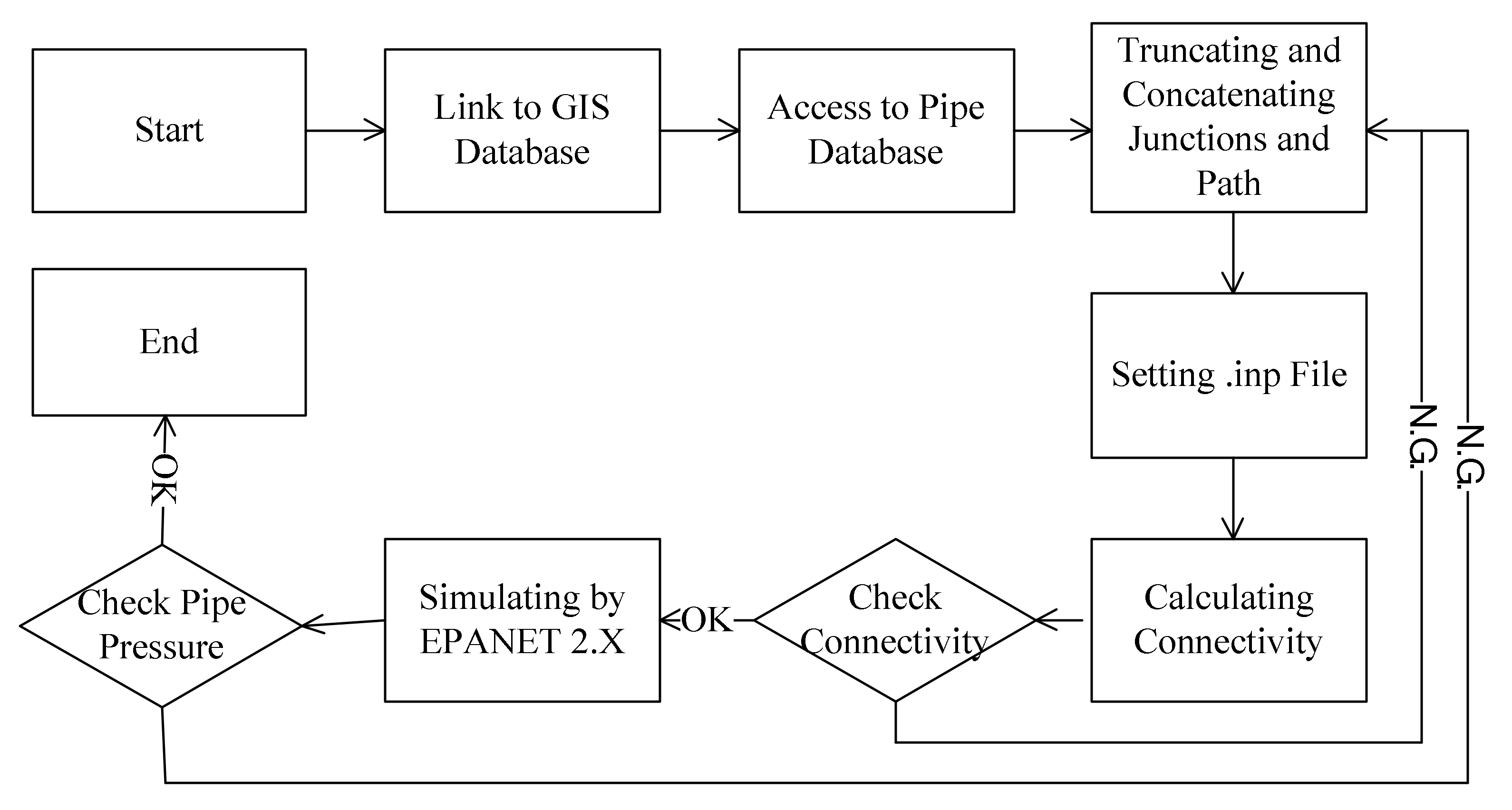
In addition, theoretically, the pipeline network roughness decreases over years of use [15]. However, due to factors, such as water pipe material, local water quality, and hydraulic gradient, the declination values need to be evaluated locally. In this study, the Hazen–Williams equation and site survey data were used to inversely calculate the roughness. For this purpose, the following process was designed, as shown in Figure 1.
2.2. The Materials
2.2.1. Introduction for the Case
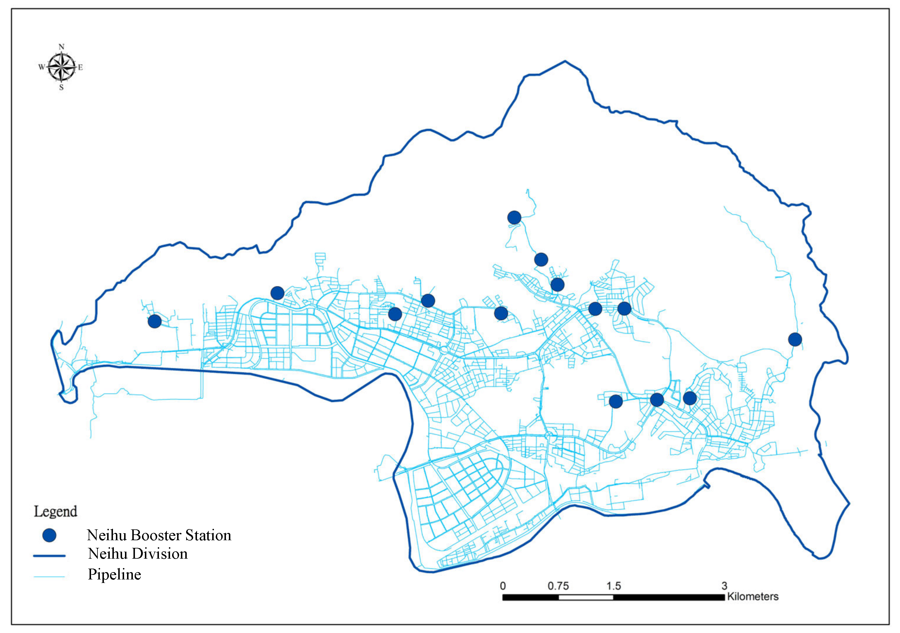
This case study was based on Taipei Water Department’s Neihu Division. The Datong Booster Station on the Dazhi Line and the Songshan Booster Station on the Neihu Line are responsible for supplying water to the Neihu Division. In addition, 15 small booster stations are responsible for supplying water to various places in the Neihu Division, as shown in Figure 2.
2.2.2. Verification of Topological Relationship
Before pretreatment, it was necessary to confirm that the connection of graph data was correct. Therefore, this study used the topology rules of graph theory for spatial relations in the geo-database to verify the data. The number of phase relation verification items and verification results could reflect whether the graph data were correct and could be used for pretreatment. The 2D and 3D spatial verification items in this study are shown in Table 1 and Table 2, respectively.
2.2.3. Pipeline Network Pretreatment in Hydrologic Analysis
The pretreatment process of the pipeline network data is shown in Figure 3. In the Figure, there are two water distribution pipelines, a water supply pipeline, a valve, and a water meter. In the second step, the start and end points of the water transmission and distribution pipelines were extracted to establish nodes, and water pipeline identity codes (WPID) at the nodes were specified. The spatial locations of other equipment were loaded to establish the node, and equipment codes were specified. Finally, a corresponding association table was established according to the connectivity.
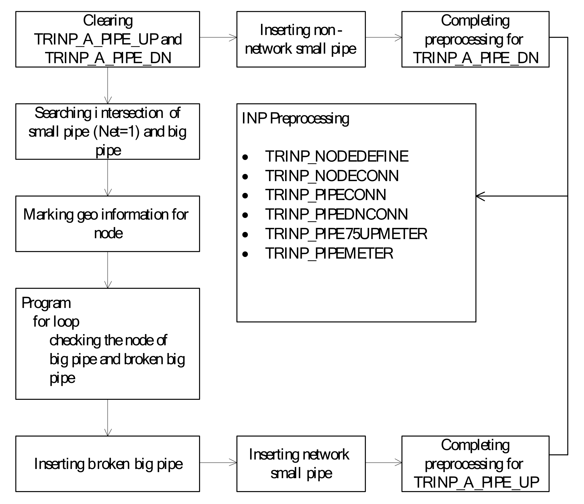
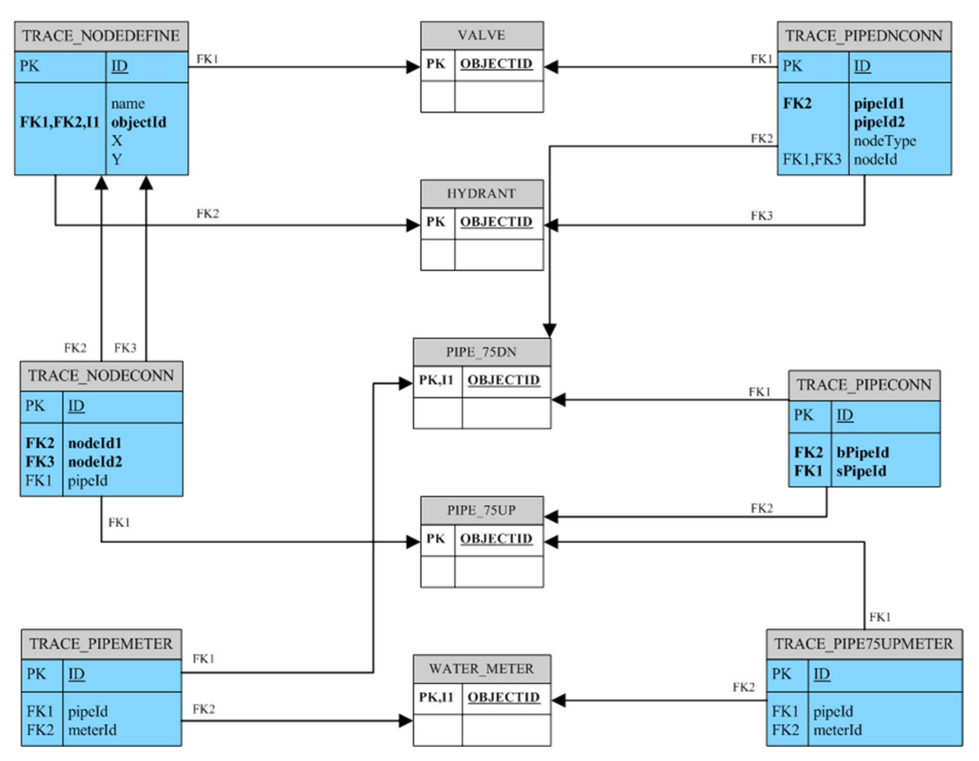
The procedures of program and database design for the input file (*.inp) are shown in Figure 4 and Figure 5. In Figure 4, the preprocessing for redefining the pipeline network structure is. The entity relationship diagram of pipeline network database is shown in Figure 5.
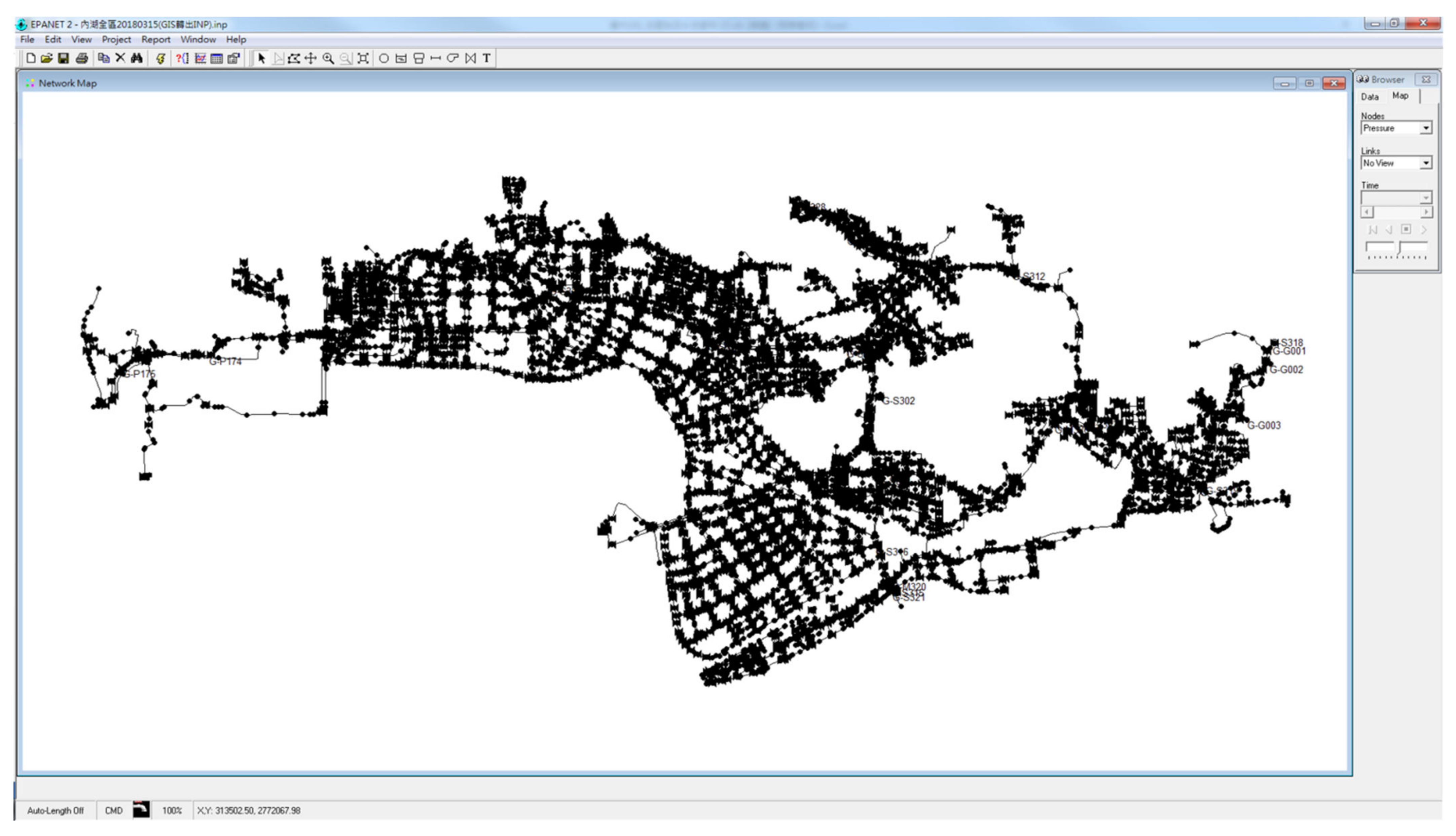
Through the above treatment and calculation, the input parameter table of the defined area could be produced (such as the EPANET 2.X input file*.inp). Figure 6 shows the INP file for Neihu Division, Taipei Water Department, and the station and equipment data collected were compared based on this file. In order to smoothly analyze the hydrologic model of the pipeline network, the parameters of the water sources (reservoir or tank), pipelines, and nodes needed to be set. After multiple iterative computations, when the calculated K(G) indicated a complete connection, the pipeline network model, as shown in Figure 6, could be obtained.
Pipe roughness is a dimensionless number. The types of pipe roughness in this study were classified as four different types. The first type is cast iron pipe. The roughness of new cast iron pipes was 130, that of 20-year-old cast iron pipes was 95, and that of 30-year-old cast iron pipes was 82.5. The interpolation approach is used to define the roughness for the two aging stages. The second type is plastic pipe. Regardless of pipe age, the roughness was 150. The third type is stainless steel pipe. The roughness of new riveted steel pipes was 110. The roughness of other pipelines was 100.
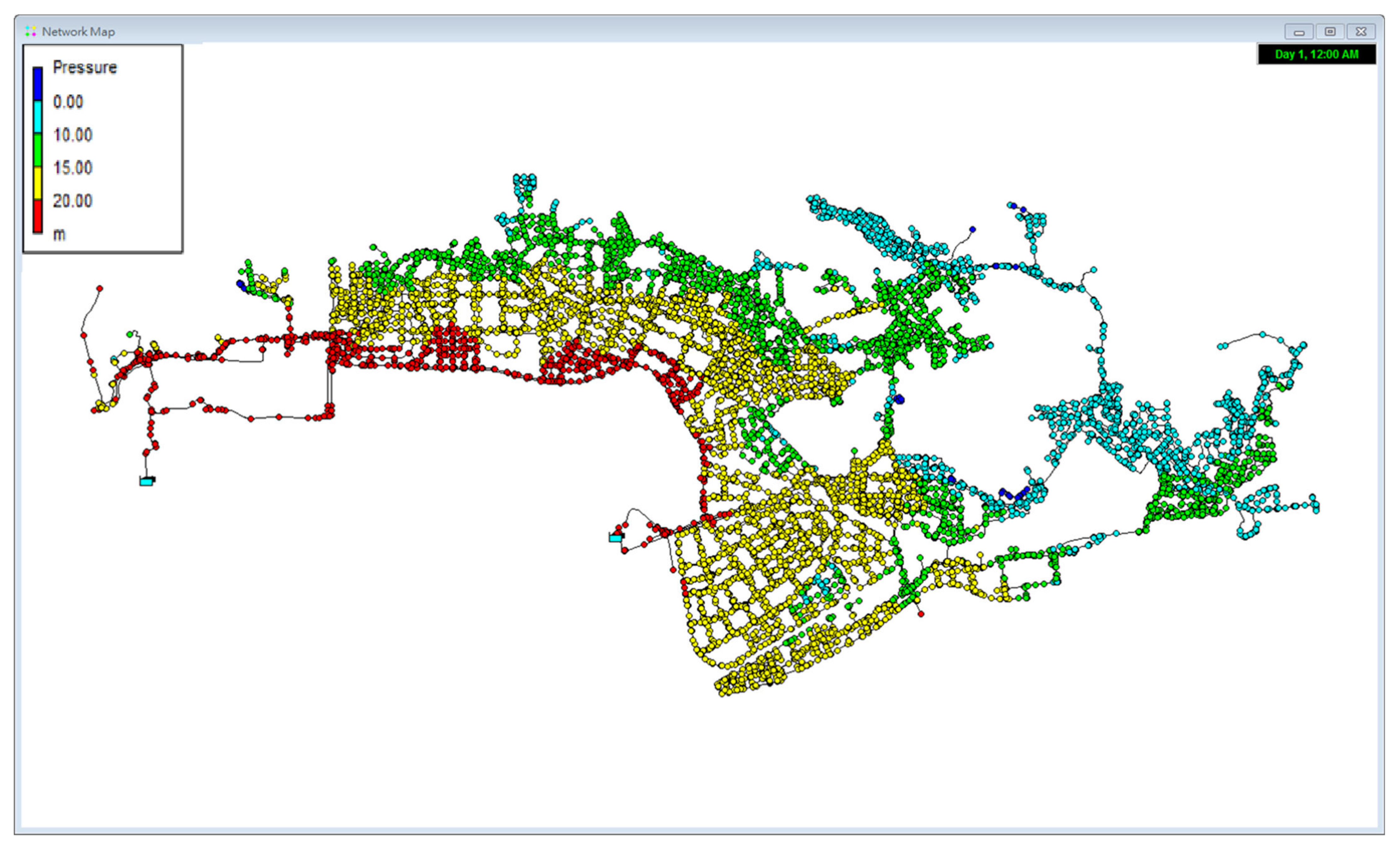
A simulation analysis was accordingly performed, and the hydrologic analysis results were used to observe the field data, such as node pressure and pipeline flow. The monitored values were applied to judge the rationality of the pipeline network model, as shown in Figure 7.
3. Results and Discussion
In order to analyze the applicability of the proposed method and judge the reliability of the proposed method, this study compared the simulation results with the WaterGEMS results and the actually measured water pressures. The Bentley WaterGEMS system provides a comprehensive yet easy-to-use decision-support tool for water distribution networks. The software improves decision makers’ operational strategies, model-building process, and can manage local model effectively. Kowalska et al. (2022) proposed the district metered areas scheme of a water distribution system for three case studies using WaterGEMS. Division of district metered areas in the existing zone of municipal water supply network was carried out using WaterGEMS. The automatic division of district metered areas facilitated and accelerated the process [16].
3.1. Comparison with WaterGEMS
3.1.1. Node Comparison
The node comparison results are shown in Table 3. Table 3 lists 16,569 confluences and compares the difference between the total head and water pressure simulated by the proposed method and WaterGEMS. As shown, there was only a small difference between the two models in the total head, whereas the majority showed no difference, indicating that the topological relationship of the pipeline network was basically the same. Therefore, it could be preliminarily determined that the method developed in this study was suitable to build a topological pipeline network model.
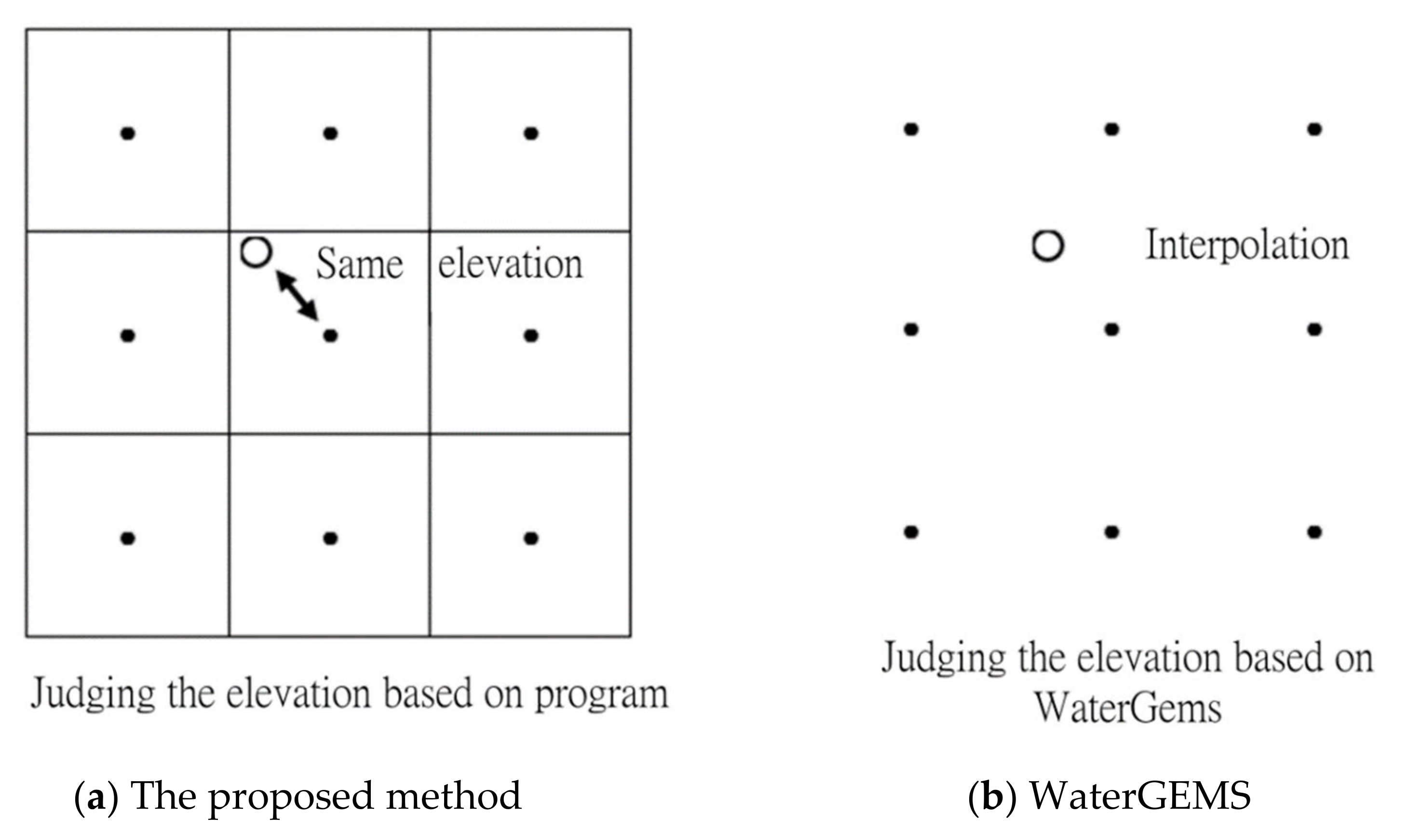
Due to the small head difference, it could be inferred that the water pressure difference was caused by the elevation difference, because WaterGEMS and the proposed method used different methods in elevation construction. As shown in Figure 8, the black spots are elevation points in the 5 m × 5 m DTM topographic map. Based on the same DTM elevation data, in the INP files of the proposed method, points within the 5 m × 5 m square had the same elevation. Meanwhile, interpolations were made using WaterGEMS according to the node coordinate positions and elevation point coordinate positions to obtain the elevation. Therefore, if a pipeline was at the junction between an embankment and a road, or at ground and mountain boundaries, the difference between the two models could be caused by the sudden rise or fall of the elevation.
The water demand distributions were the same at more than 99% of the nodes. It could be inferred that the proposed method was reliable in judging the pipeline closest to the water meter and equally distributing water to the front and rear nodes. However, water demands were still different at some nodes, and the detailed observation of these nodes showed that there were two causes, as follows:
- (1)
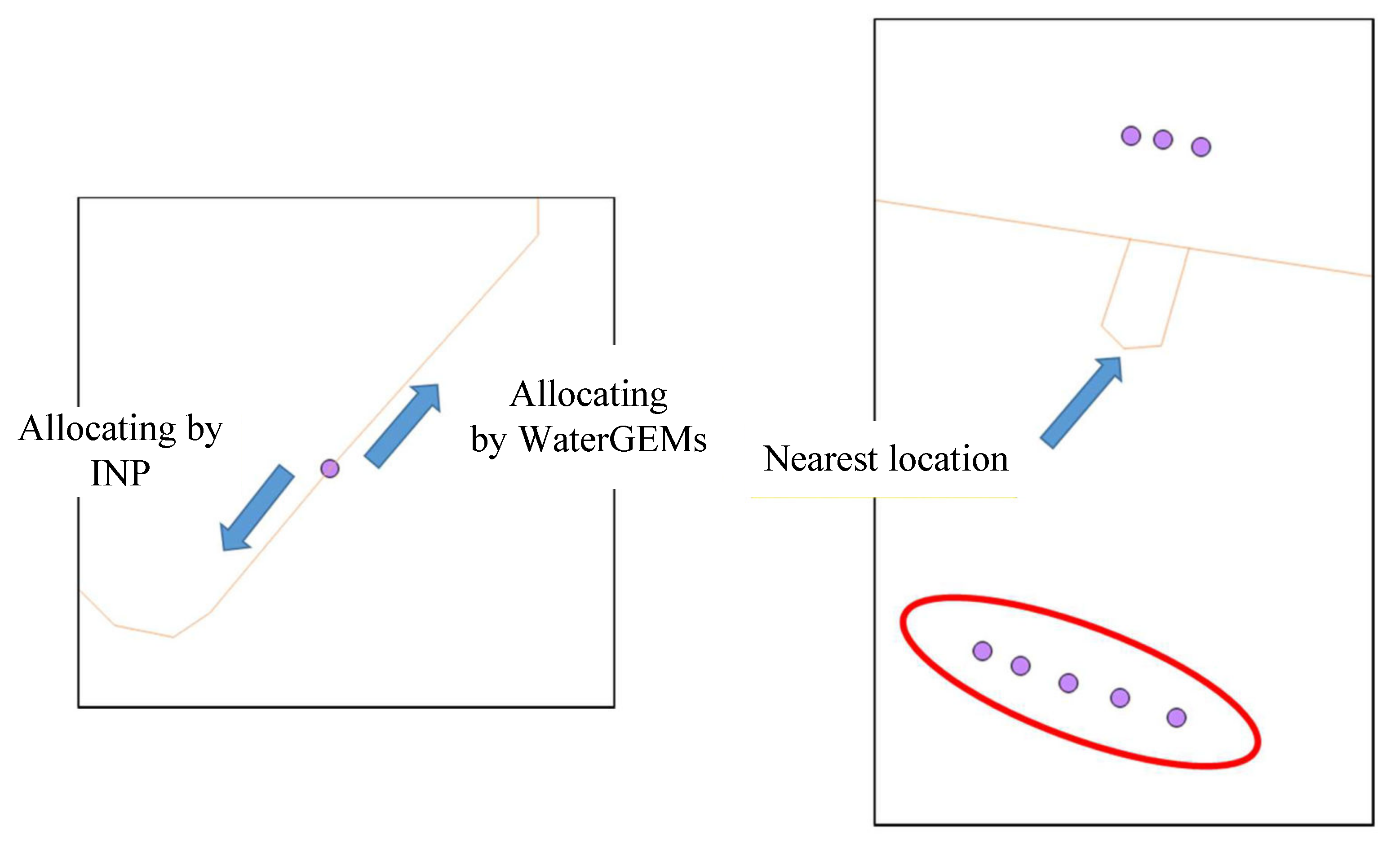
- The water meter was located on the pipeline and connected by the front and rear pipelines. Using the proposed method and WaterGEMS to distribute water to the front and rear pipelines would result in different water demands at the nodes, as shown in the picture on the left of Figure 9.
- (2)
- As shown in the right picture of Figure 9, the pipeline closest to the circled water meter was connected by two pipelines, so the proposed method and WaterGEMS might have distributed water to different pipelines.
Figure 9.
Causes of the differences in water demand distribution.

3.1.2. Pipeline Comparison
The pipeline comparison table (Table 4) showed that about 94% of the pipeline flow differences in the model were below 1 CMD, and more than 99% of the pipeline flow differences were below 10 CMD.
3.2. In-Situ Water Pressure Measurements
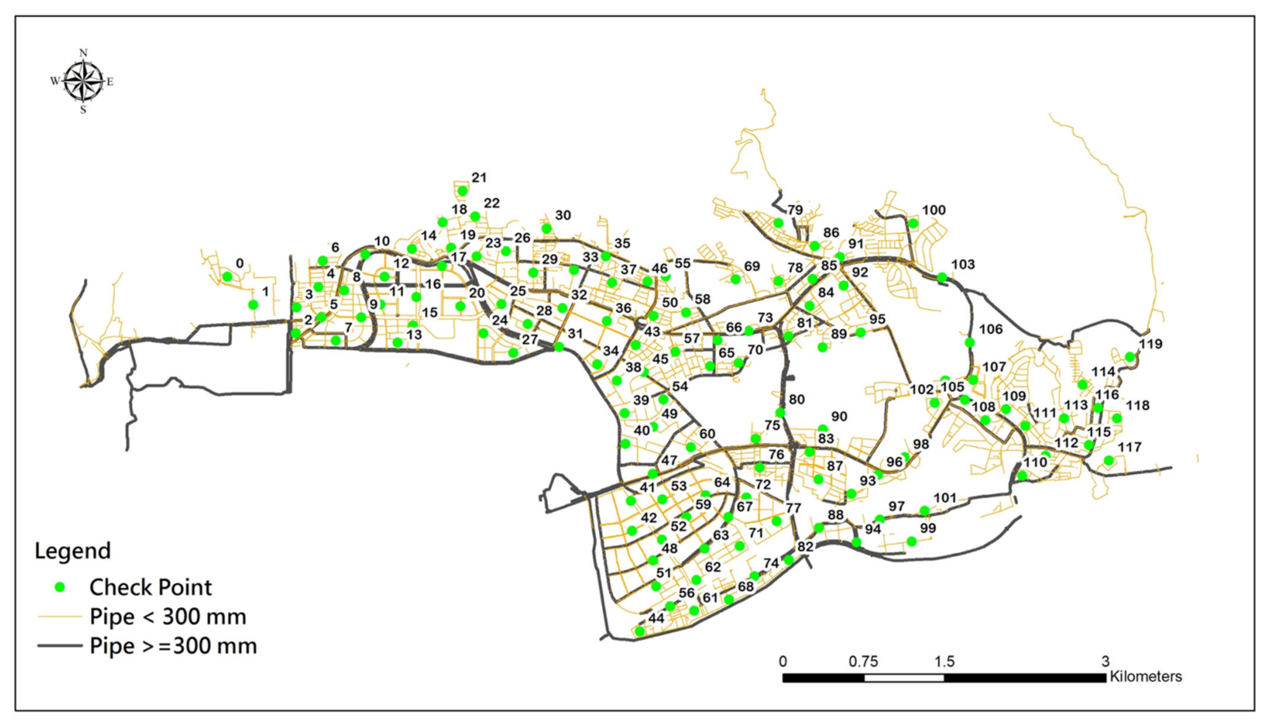
A total of 120 fire hydrants were used for the water pressure measurements in this study. In order to maximize the efficiency of the site measurements and model corrections, fire hydrants were first removed from the water supply areas of all small booster stations. The selected results are shown in Figure 10.
3.3. Comparison between Simulation and Actual Measurement
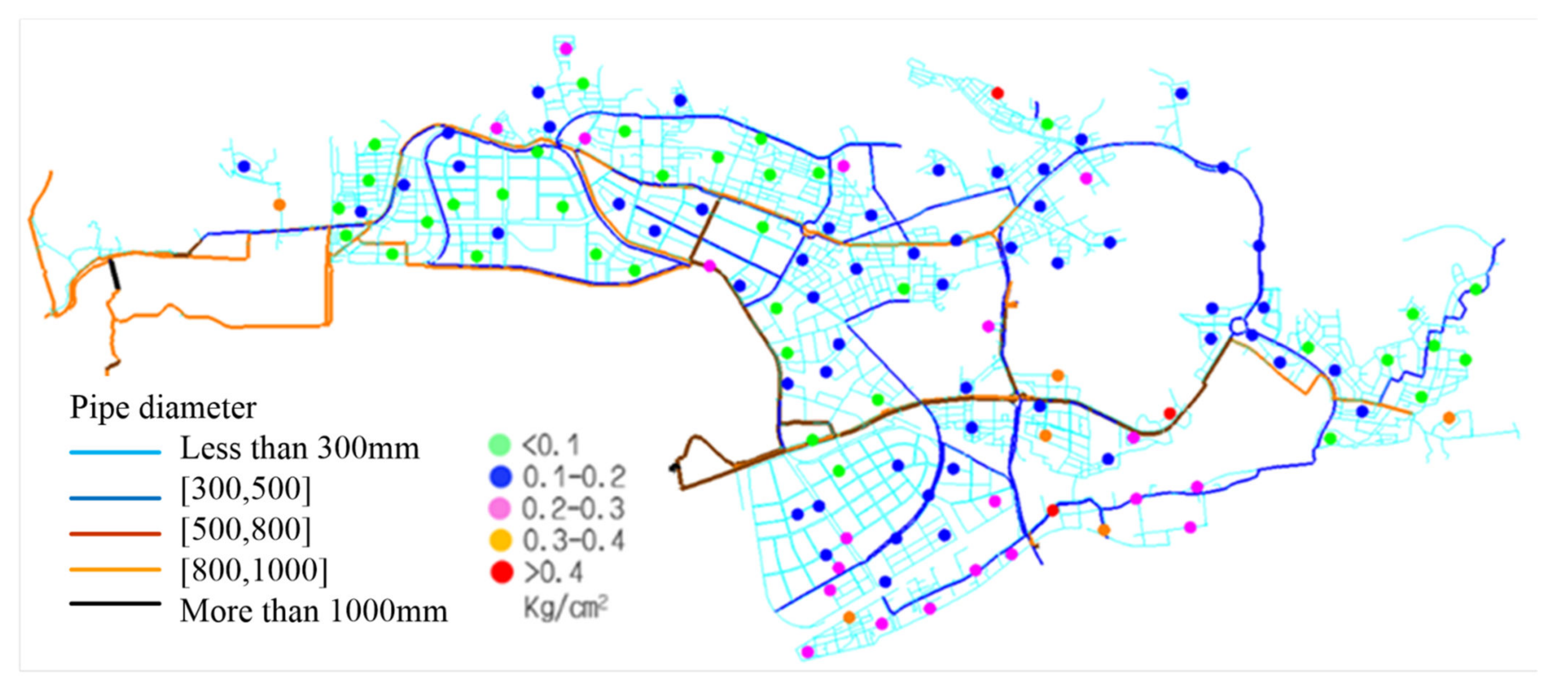
The analysis of the results of the hydrologic model compared the simulated water pressure and the actual measured water pressure of the nodes representing fire hydrants in the model. According to the analysis results shown in Table 5, among the 120 water pressure measurement points, 35 had a differential pressure below 0.1 kg/cm2, 54 had a differential pressure between 0.1 and 0.2 kg/cm2, 22 had a differential pressure between 0.2 and 0.3 kg/cm2, and 9 had a differential pressure of above 0.3 kg/cm2. A total of 100 points had an error of less than 20%, accounting for 83.3% of the 120 measurement points. The calculated correlation coefficient between the mean value observed and the simulated pressure was 0.959. Compared with similar studies in the literature [17], the correlation can be considered as good. It was adopted, based on the calibration that the developed model was acceptable and represented a reliable representation of the tested water supply network. The points in the differential pressure distribution are shown in Figure 11.
4. Conclusions
The proposed method could be used to quickly build a hydrologic model of a pipeline network, as well as to quickly and accurately update the hydrologic model for analysis by simply modifying the GIS graph data and equipment management system.
In order to calibrate the rationality of the pipeline network model built by the proposed method, the results were compared with the WaterGEMS analysis. The results show a high consistency in the pipeline network topology, pipeline crossover, and node disposition. The differences in elevation and water demand distribution at some nodes were caused by special terrain and water meter positions, indicating that the model built by the proposed method had high reliability. This article proposed a modified approach based on integrating the graph theory, GIS database, and an open source system, such as EPANET, for a cheaper and acceptable solution for urban water resource management.
After the INP file was opened in the hydraulic analysis software, the model used simple settings and processing steps to make analyses, which met the requirements of the Taipei Water Department for automated model construction. Moreover, according to the preliminary analysis results of the hydrologic model, the water pressure calculated by the Neihu Division model was distributed within a reasonable range, indicating that the analysis model could be used in future work programs. When building future hydraulic analysis models, users only need to refer to the processes and procedures specified in this report to quickly build a preliminary hydrologic analysis model and then adjust parameters according to the target requirements.
The effectiveness of the proposed method in the analysis on different grid sizes, local variables, and climate extremes is still unknown, and need to be further investigated. In the future, the proposed method could be promoted for use in urban water management systems of a smart city, and the differences could be analyzed.
Author Contributions
C.-C.S.: Conceptualization, Investigation, Data collection, Programming, Software design. T.C.: Methodology, Writing-Original draft preparation. C.-C.C.: Visualization, Writing-Reviewing and Editing. All authors have read and agreed to the published version of the manuscript.
Funding
This research was supported in part by the Ministry of Science and Technology, Taiwan, ROC. Under Grant numbers 110-2221-E-507-005 and 111-2221-E-507-002.
Conflicts of Interest
The authors declare no conflict of interest.
References
- United Nations. The United Nations World Water Development Report 2015: Water for a Sustainable World; United Nations Educational; Scientific and Cultural Organization (UNESCO): Paris, France, 2015. [Google Scholar]
- United Nations. Transforming Our World: The 2030 Agenda for Sustainable Development; United Nations: New York, NY, USA, 2016. [Google Scholar]
- Chartzoulakis, K.S.; Paranychianakis, N.V.; Angelakis, A.N. Water resources management in the Island of Crete, Greece, with emphasis on the agricultural use. Water Policy 2001, 3, 193–205. [Google Scholar] [CrossRef]
- Lee, C.-C.; Huang, K.-C.; Kuo, S.-Y.; Cheng, C.-K.; Tung, C.-P.; Liu, T.-M. Climate change research in Taiwan: Beyond following the mainstream. Environ. Hazards 2022, 1–19. [Google Scholar] [CrossRef]
- Taipei Water Department. Taipei Water Department Statistical Yearbook 2021; Taipei Water Department: Taipei, Taiwan, 2022. [Google Scholar]
- Sample, D.J.; Heaney, J.P.; Wright, L.T.; Koustas, R. Geographic information systems, decision support systems, and urban storm-water management. J. Water Resour. Plan. Manag. 2001, 127, 155–161. [Google Scholar] [CrossRef]
- Abdelhaleem, F.S.; Basiouny, M.; Ashour, E.; Mahmoud, A. Application of remote sensing and geographic information systems in irrigation water management under water scarcity conditions in Fayoum, Egypt. J. Environ. Manag. 2021, 299, 113683. [Google Scholar] [CrossRef] [PubMed]
- Figueiredo, I.; Esteves, P.; Cabrita, P. Water wise–a digital water solution for smart cities and water management entities. Procedia Comput. Sci. 2021, 181, 897–904. [Google Scholar] [CrossRef]
- Gheibi, M.; Emrani, N.; Eftekhari, M.; Behzadian, K.; Mohtasham, M.; Abdollahi, J. Assessing the failures in water distribution networks using a combination of geographic information system, EPANET 2, and descriptive statistical analysis: A case study. Sustain. Water Resour. Manag. 2022, 8, 47. [Google Scholar] [CrossRef]
- Grayman, W.M. History of water quality modeling in distribution systems. In Proceedings of the WDSA/CCWI Joint Conference Proceedings, Kingston, ON, Canada, 23–25 July 2018. [Google Scholar]
- Savić, D.; Mala-Jetmarova, H. History of Optimization in Water Distribution System Analysis. In Proceedings of the WDSA/CCWI Joint Conference Proceedings, Kingston, ON, Canada, 23–25 July 2018. [Google Scholar]
- Xu, T.; Liang, F. Machine learning for hydrologic sciences: An introductory overview. Wiley Interdisciplinary Reviews. Water 2021, 8, e1533. [Google Scholar] [CrossRef]
- Abhijith, G.R.; Ostfeld, A. Contaminant fate and transport modeling in distribution systems: EPANET-C. Water 2022, 14, 1665. [Google Scholar] [CrossRef]
- West, D.B. Introduction to Graph Theory; Pearson College: Victoria, BC, Canada, 2000. [Google Scholar]
- Seifollahi-Aghmiuni, S.; Bozorg Haddad, O.; Omid, M.H.; Mariño, M.A. Effects of pipe roughness uncertainty on water distribution network performance during its operational period. Water Resour. Manag. 2013, 27, 1581–1599. [Google Scholar] [CrossRef]
- Kowalska, B.; Suchorab, P.; Kowalski, D. Division of district metered areas (DMAs) in a part of water supply network using WaterGEMS (Bentley) software: A case study. Appl. Water Sci. 2022, 12, 1–10. [Google Scholar] [CrossRef]
- Kepa, U. Use of the hydraulic model for the operational analysis of the water supply network: A case Study. Water 2021, 13, 326. [Google Scholar] [CrossRef]
Figure 1.
Pipeline network construction and connectivity verification process.

Figure 2.
Neihu Division water supply map.

Figure 3.
Description of the automated logic diagram of the pretreatment process.

Figure 4.
Database calculation and treatment flow chart.

Figure 5.
Association of database results.

Figure 6.
Pipeline network of Neihu Division, Taipei Water Department.

Figure 7.
Simulated water pressure analysis of the Neihu pipeline network node (in meters).

Figure 8.
Differences in elevation calculated by two methods.

Figure 10.
Actual water pressure measurement points.

Figure 11.
Points in the differential pressure distribution.


Table 1.
2D spatial verification items.
| Item | Device Type | |||||||
|---|---|---|---|---|---|---|---|---|
| Type of graph data | Water distribution pipe Water supply pipe Hot spring pipe | Water meter | Accessory equipment | Valve | Bolt | Manhole | Cabinet | Water distribution pipe, water supply pipe, hot spring pipe, water meter, accessory equipment, cabinet, valve, bolt, manhole |
| 2D inspection logic | Pipeline endpoints should be a piece of equipment (pipe cap, water meter) | Disconnected from pipeline | Data repeatability | |||||
| Self-intersected pipeline | ||||||||
| Suspended pipeline | ||||||||
| Example |  |  |  | |||||
Table 2.
3D spatial verification items.
| Item | Device Type | ||||||
|---|---|---|---|---|---|---|---|
| Graph data inspection | Water distribution pipe Water supply pipe Hot spring pipe | Water meter | Accessory equipment | Valve | Bolt | Manhole | Cabinet |
| 3D inspection logic | z of pipeline node is 0 | Inspect whether the equipment coordinate z is consistent with the pipeline endpoint | Inspect whether the measurement point is greatly different from the DTM | ||||
| z of pipeline node is negative | |||||||
| The elevation at common points of pipelines are different | |||||||
| Inspect whether the measurement point is greatly different from the DTM | |||||||
| The elevation difference between the previous and next points is 3 m | |||||||
| Example |  |  |  | ||||
Table 3.
Model node comparison between the proposed method and WaterGEMS.
| The Differences of Total Head (Meter) | The Differences of Pressure (Meter) | ||
|---|---|---|---|
| Value | Rate | Value | Rate |
| Equal 0 | 72.33% | Less than 1 | 99.14% |
| Less than 1 | 27.67% | Equal, more than 1 and less than 6 | 0.86% |
Table 4.
Model pipeline comparison.
| Pipeline Flow Difference (m3/Day) | Rate |
|---|---|
| [0~1] | 94.11% |
| [1~10] | 5.51% |
| [10~50] | 0.30% |
| [50~200] | 0.07% |
| [200~400] | 0.01% |
Table 5.
Differential pressure statistics between simulation and actual measurement.
| Water Pressure Differences (kg/cm2) | Percentage (%) | Error (%) | Percentage (%) |
|---|---|---|---|
| [0~0.1] | 29.2 | 10 | 55 |
| [0.1~0.2] | 45.0 | 10–20 | 28.3 |
| [0.2~0.4] | 18.3 | More than 20 | 16.7 |
| More than 0.4 | 7.5 | - | - |
Publisher’s Note: MDPI stays neutral with regard to jurisdictional claims in published maps and institutional affiliations. |
© 2022 by the authors. Licensee MDPI, Basel, Switzerland. This article is an open access article distributed under the terms and conditions of the Creative Commons Attribution (CC BY) license (https://creativecommons.org/licenses/by/4.0/).
Share and Cite
MDPI and ACS Style
Shiu, C.-C.; Chiang, T.; Chung, C.-C. A Modified Hydrologic Model Algorithm Based on Integrating Graph Theory and GIS Database. Water 2022, 14, 3000. https://doi.org/10.3390/w14193000
AMA Style
Shiu C-C, Chiang T, Chung C-C. A Modified Hydrologic Model Algorithm Based on Integrating Graph Theory and GIS Database. Water. 2022; 14(19):3000. https://doi.org/10.3390/w14193000
Chicago/Turabian StyleShiu, Chia-Cheng, Tzuping Chiang, and Chih-Chung Chung. 2022. "A Modified Hydrologic Model Algorithm Based on Integrating Graph Theory and GIS Database" Water 14, no. 19: 3000. https://doi.org/10.3390/w14193000
Note that from the first issue of 2016, this journal uses article numbers instead of page numbers. See further details here.