
Flood Inundation Modeling by Integrating HEC–RAS and Satellite Imagery: A Case Study of the Indus River Basin
 , ,
, ,  , and
, and
Abstract
:1. Introduction
2. Materials and Methods
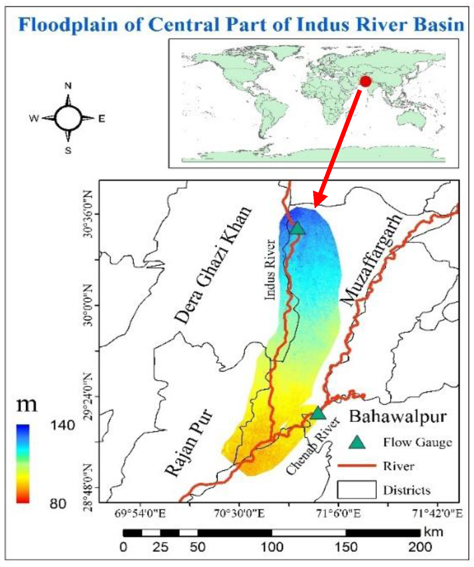
2.1. Study Area
2.2. Datasets Used in the Study
2.3. Numerical Simulation in the HEC–RAS Model
2.4. Satellite-Based Flood Extent Mapping

| Satellite Datasets | Method | Threshold Values | References |
|---|---|---|---|
| Landsat 5 TM | NDWI (2,4) MNDWI 1 (2,5) | 0.234, 0.205 0.35, 0.45, 0.33 | [137,138] [135,137,139] |
| Landsat 8 OLI | NDWI (3,5) MNDWI 1 (3,6) MNDWI 2 (3,7) | 0.113, 0.09 0.286, 0.33, 0.25–0.31 0.462 | [137,139] [139,140,141] [140] |
| MODIS (MOD09GA/MOD09A1) | NDWI (4,2) MNDWI 1 (4,6) | 0.0 0.44, 0.34 | [142] [143,144] |
2.5. Calibration and Validation of HEC–RAS Model
2.6. Accuracy Assessment of HEC–RAS Model
3. Results
3.1. Land Use of the Study Area
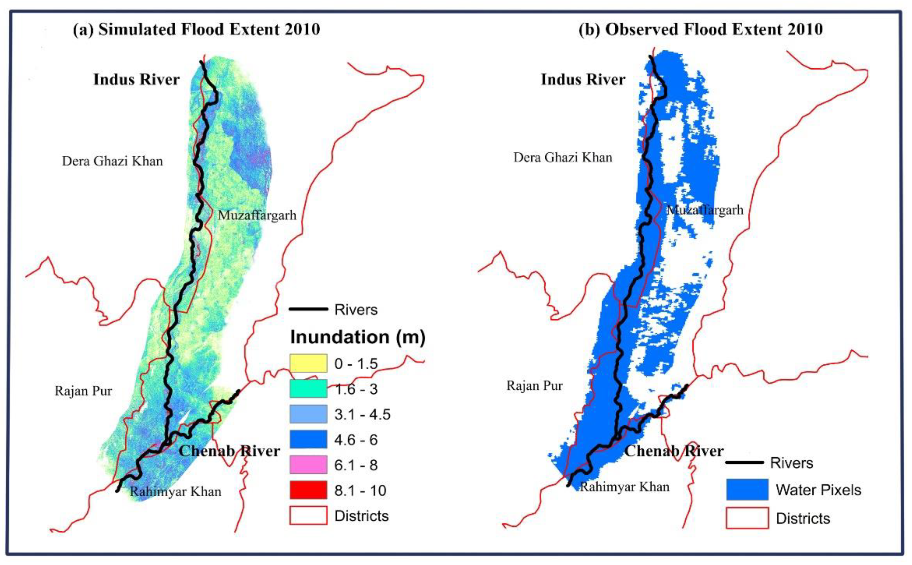
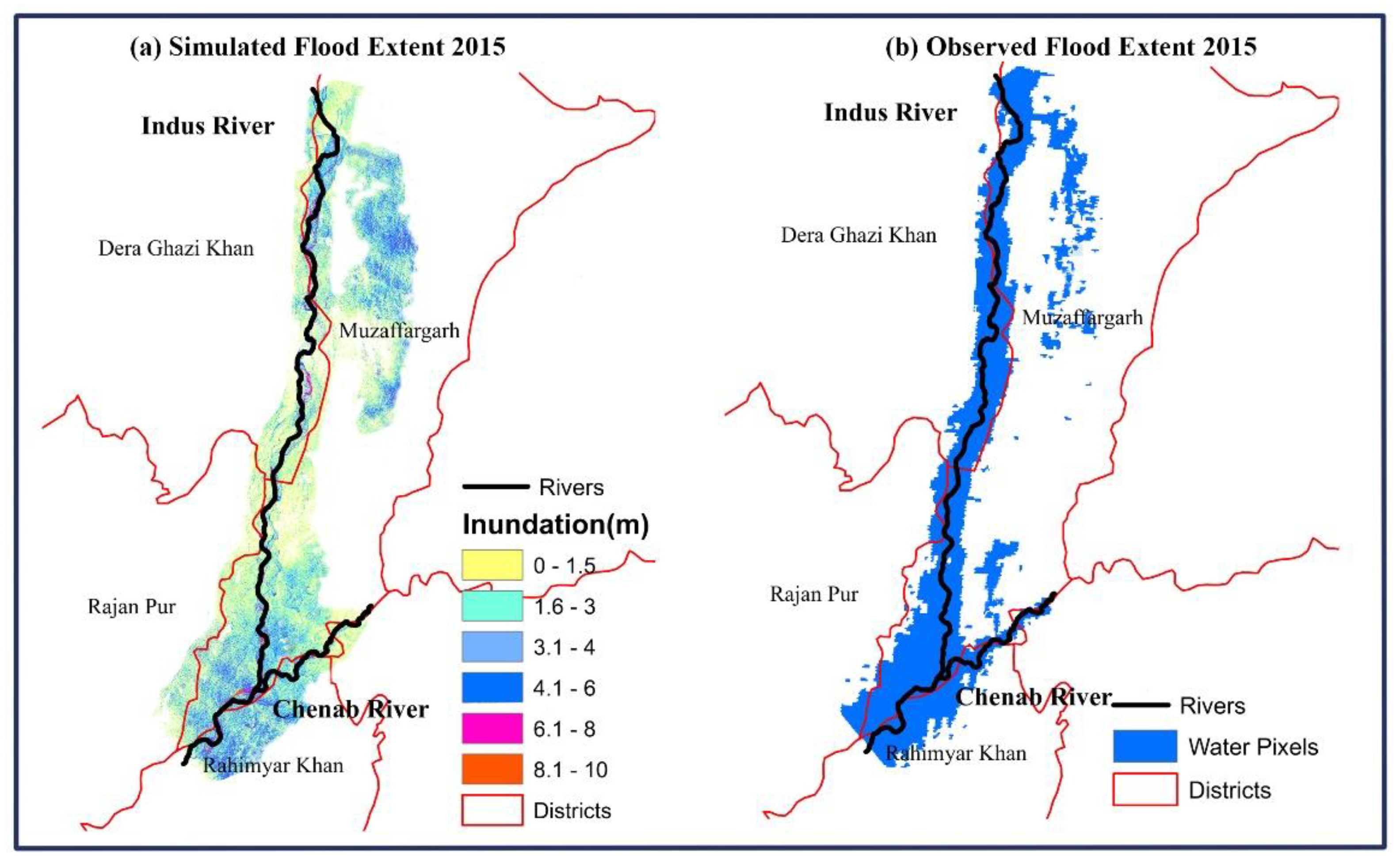
3.2. Performance Evaluation of HEC–RAS Model
4. Discussion
5. Conclusions
Supplementary Materials
Author Contributions
Funding
Institutional Review Board Statement
Informed Consent Statement
Data Availability Statement
Conflicts of Interest
References
- Neumayer, E.; Plümper, T. The gendered nature of natural disasters: The impact of catastrophic events on the gender gap in life expectancy, 1981–2002. Ann. Assoc. Am. Geogr. 2007, 97, 551–566. [Google Scholar] [CrossRef]
- Cannon, T. Vulnerability analysis and the explanation of ‘natural’disasters. Disasters Dev. Environ. 1994, 1, 13–30. [Google Scholar]
- Ashley, S.T.; Ashley, W.S. Flood fatalities in the United States. J. Appl. Meteorol. Climatol. 2008, 47, 805–818. [Google Scholar] [CrossRef]
- Seyedeh, S.; Thamer, A.; Mahmud, A.; Majid, K.; Amir, S. Integrated Modelling for Flood Hazard Mapping Using Watershed Modelling System. Am. J. Eng. Appl. Sci. 2008, 1, 149–156. [Google Scholar]
- Stefanidis, S.; Stathis, D. Assessment of flood hazard based on natural and anthropogenic factors using analytic hierarchy process (AHP). Nat. Hazards 2013, 68, 569–585. [Google Scholar] [CrossRef]
- Alfieri, L.; Cohen, S.; Galantowicz, J.; Schumann, G.J.; Trigg, M.A.; Zsoter, E.; Prudhomme, C.; Kruczkiewicz, A.; de Perez, E.C.; Flamig, Z.; et al. A global network for operational flood risk reduction. Environ. Sci. 2018, 84, 149–158. [Google Scholar] [CrossRef]
- IRFC. World Disasters Report, 2003; International Federation of Red Cross and Red Crescent Societies: Geneva, Switzerland, 2003. [Google Scholar]
- ARDC. Natural Disaster Data Book 2009 (an Analytical Review); Asia Disaster Reduction Center: Kobe, Japan, 2009; p. 23. [Google Scholar]
- Jongman, B.; Ward, P.J.; Aerts, J.C. Global exposure to river and coastal flooding: Long term trends and changes. Glob. Environ. Change 2012, 22, 823–835. [Google Scholar] [CrossRef]
- Munich, R. NatCatSERVICE Loss Events Worldwide 1980–2014; Munich Reinsurance: Munich, Germany, 2015; p. 10. [Google Scholar]
- Jonkman, S.N. Global perspectives on loss of human life caused by floods. Nat. Hazards 2005, 34, 151–175. [Google Scholar] [CrossRef]
- Savage, J.T.S.; Bates, P.; Freer, J.; Neal, J.; Aronica, G. When does spatial resolution become spurious in probabilistic flood inundation predictions? Hydrol. Process. 2016, 30, 2014–2032. [Google Scholar] [CrossRef]
- Messner, F.; Meyer, V. Flood damage, vulnerability and risk perception—Challenges for flood damage research. In Flood Risk Management: Hazards, Vulnerability and Mitigation Measures; Springer: Dordrecht, The Netherlands, 2006; pp. 149–167. [Google Scholar]
- Dutta, D.; Herath, S.; Musiake, K. A mathematical model for flood loss estimation. J. Hydrol. 2003, 277, 24–49. [Google Scholar] [CrossRef]
- Belletti, B.; Dufour, S.; Piégay, H. What is the relative effect of space and time to explain the braided river width and island patterns at a regional scale? River Res. Appl. 2015, 31, 1–15. [Google Scholar] [CrossRef]
- UNESCO. Water: A Shared Responsibility; The United Nations World Water Development Report 2, World Water Assessment Programme; UNESCO: Paris, France, 2006. [Google Scholar]
- Razavi, S.; Gober, P.; Maier, H.R.; Brouwer, R.; Wheater, H. Anthropocene flooding: Challenges for science and society. Hydrol. Process. 2020, 34, 1996–2000. [Google Scholar] [CrossRef] [Green Version]
- FFC. Annual Flood Report, Federal Flood Commission, Ministry of Water and Power of Pakistan; Water and Power Development Authority: Islamabad, Pakistan, 2017.
- FFC. Annual Flood Report, Federal Flood Commission, Ministry of Water and Power of Pakistan; Water and Power Development Authority: Islamabad, Pakistan, 2018.
- FFC. Annual Flood Report, Federal Flood Commission, Ministry of Water and Power of Pakistan; Water and Power Development Authority: Islamabad, Pakistan, 2020.
- FFC. Annual Flood Report, Federal Flood Commission, Ministry of Water and Power of Pakistan; Water and Power Development Authority: Islamabad, Pakistan, 2014.
- Archer, D.R.; Forsythe, N.; Fowler, H.J.; Shah, S.M. Sustainability of water resources management in the Indus Basin under changing climatic and socio economic conditions. Hydrol. Earth Syst. Sci. 2010, 14, 1669–1680. [Google Scholar] [CrossRef]
- Biswas, A.K. Indus water treaty: The negotiating process. Water Int. 1992, 17, 201–209. [Google Scholar] [CrossRef]
- Sohail, M.T.; Delin, H.; Siddiq, A. Indus basin waters a main resource of water in Pakistan: An analytical approach. Curr. World Environ. 2014, 9, 670. [Google Scholar] [CrossRef]
- Das, T.; Maurer, E.P.; Pierce, D.W.; Dettinger, M.D.; Cayan, D.R. Increases in flood magnitudes in California under warming climates. J. Hydrol. 2013, 501, 101–110. [Google Scholar] [CrossRef]
- Field, C.B.; Barros, V.; Stocker, T.F.; Dahe, Q. Managing the Risks of Extreme Events and Disasters to Advance Climate Change Adaptation: Special Report of the Intergovernmental Panel on Climate Change; Cambridge University Press: Cambridge, UK, 2012. [Google Scholar]
- Visser, H.; Petersen, A.C.; Ligtvoet, W. On the relation between weather-related disaster impacts, vulnerability and climate change. Clim. Chang. 2014, 125, 461–477. [Google Scholar] [CrossRef]
- Arnell, N.W.; Gosling, S.N. The impacts of climate change on river flood risk at the global scale. Clim. Chang. 2016, 134, 387–401. [Google Scholar] [CrossRef]
- Alfieri, L.; Burek, P.; Feyen, L.; Forzieri, G. Global warming increases the frequency of river floods in Europe. Hydrol. Earth Syst. Sci. 2015, 19, 2247–2260. [Google Scholar] [CrossRef]
- Lehner, B.; Döll, P.; Alcamo, J.; Henrichs, T.; Kaspar, F. Estimating the impact of global change on flood and drought risks in Europe: A continental, integrated analysis. Clim. Chang. 2006, 75, 273–299. [Google Scholar] [CrossRef]
- Plate, E.J. Flood risk and flood management. J. Hydrol. 2002, 267, 2–11. [Google Scholar] [CrossRef]
- Luo, P.; He, B.; Duan, W.; Takara, K.; Nover, D. Impact assessment of rainfall scenarios and land-use change on hydrologic response using synthetic Area IDF curves. J. Flood Risk Manag. 2018, 11, S84–S97. [Google Scholar] [CrossRef]
- Stoffel, M.; Wyżga, B.; Marston, R.A. Floods in mountain environments: A synthesis. Geomorphology 2016, 272, 1–9. [Google Scholar] [CrossRef]
- Krapesch, G.; Hauer, C.; Habersack, H. Scale orientated analysis of river width changes due to extreme flood hazards. Nat. Hazards Earth Syst. Sci. 2011, 11, 2137–2147. [Google Scholar] [CrossRef]
- Dean, D.J.; Schmidt, J.C. The geomorphic effectiveness of a large flood on the Rio Grande in the Big Bend region: Insights on geomorphic controls and post-flood geomorphic response. Geomorphology 2013, 201, 183–198. [Google Scholar] [CrossRef]
- Grove, J.R.; Croke, J.; Thompson, C. Quantifying different riverbank erosion processes during an extreme flood event. Earth Surf. Process. Landf. 2013, 38, 1393–1406. [Google Scholar] [CrossRef]
- Surian, N.; Righini, M.; Lucía, A.; Nardi, L.; Amponsah, W.; Benvenuti, M.; Borga, M.; Cavalli, M.; Comiti, F.; Marchi, L. Channel response to extreme floods: Insights on controlling factors from six mountain rivers in northern Apennines, Italy. Geomorphology 2016, 272, 78–91. [Google Scholar] [CrossRef]
- Fread, D.L. Flow routing. In Handbook of Hydrology; McGraw-Hill: New York, NY, USA, 1992; Chapter 10; pp. 316–345. [Google Scholar]
- Kundzewicz, Z.W.; Kaczmarek, Z. Coping with hydrological extremes. Water Int. 2000, 25, 66–75. [Google Scholar] [CrossRef]
- Ebert, A.; Kerle, N.; Stein, A. Urban social vulnerability assessment with physical proxies and spatial metrics derived from air-and spaceborne imagery and GIS data. Nat. Hazards 2009, 48, 275–294. [Google Scholar] [CrossRef]
- Ali, S.; Masud Cheema, M.J.; Bakhsh, A.; Khaliq, T. Near real time flood forecasting in the transboundary Chenab river using Global Satellite Mapping of Precipitation. Pak. J. Agric. Sci. 2020, 57, 1327–1335. [Google Scholar]
- Ranzi, R.; Mazzoleni, M.; Milanesi, L.; Pilotti, M.; Ferri, M.; Giuriato, F.; Michel, G.; Fewtrell, T.; Bates, P.D.; Neal, J. Critical review of non-structural measures for water-related risks. In KULTURisk; UNESCO-IHE: Delft, The Netherlands, 2011; p. 42. [Google Scholar]
- Chiang, P.; Willems, P.; Berlamont, J. A conceptual river model to support real-time flood control (Demer River, Belgium). In Proceedings of the River Flow 2010 International Conference on Fluvial Hydraulics, TU Braunschweig, Braunschweig, Germany, 8–10 September 2010; pp. 8–10. [Google Scholar]
- Wu, J.; Liu, H.; Wei, G.; Song, T.; Zhang, C.; Zhou, H. Flash flood forecasting using support vector regression model in a small mountainous catchment. Water 2019, 11, 1327. [Google Scholar] [CrossRef]
- Xiao, Z.; Liang, Z.; Li, B.; Hou, B.; Hu, Y.; Wang, J. New flood early warning and forecasting method based on similarity theory. J. Hydrol. Eng. 2019, 24, 04019023. [Google Scholar] [CrossRef]
- Chu, H.; Wu, W.; Wang, Q.; Nathan, R.; Wei, J. An ANN-based emulation modelling framework for flood inundation modelling: Application, challenges and future directions. Environ. Model. Softw. 2020, 124, 104587. [Google Scholar] [CrossRef]
- Gichamo, T.Z.; Popescu, I.; Jonoski, A.; Solomatine, D. River cross-section extraction from the ASTER global DEM for flood modeling. Environ. Model. Softw. 2012, 31, 37–46. [Google Scholar] [CrossRef]
- Shamaoma, H.; Kerle, N.; Alkema, D. Extraction of flood-modelling related base-data from multi-source remote sensing imagery. In Proceedings of the ISPRS Mid-Term Symposium, Enschede, The Netherlands, 8–11 May 2006. [Google Scholar]
- Hunter, N.M.; Bates, P.D.; Horritt, M.S.; Wilson, M.D. Simple spatially-distributed models for predicting flood inundation: A review. Geomorphology 2007, 90, 208–225. [Google Scholar] [CrossRef]
- Horritt, M.; Bates, P. Evaluation of 1D and 2D numerical models for predicting river flood inundation. J. Hydrol. 2002, 268, 87–99. [Google Scholar] [CrossRef]
- Pappenberger, F.; Beven, K.J.; Hunter, N.; Bates, P.; Gouweleeuw, B.; Thielen, J.; De Roo, A. Cascading model uncertainty from medium range weather forecasts (10 days) through a rainfall-runoff model to flood inundation predictions within the European Flood Forecasting System (EFFS). Hydrol. Earth Syst. Sci. Discuss. 2005, 9, 381–393. [Google Scholar] [CrossRef]
- Smirnov, S.; Werner, W. Critical exponents for two-dimensional percolation. arXiv 2001, arXiv:math/0109120v2. [Google Scholar] [CrossRef]
- Leon, A.S.; Goodell, C. Controlling hec-ras using matlab. Environ. Model. Softw. 2016, 84, 339–348. [Google Scholar] [CrossRef]
- Dyhouse, G.; Hatchett, J.; Benn, J. Floodplain Modeling Using HEC-RAS; Haestad Press: Watertown, CT, USA, 2003. [Google Scholar]
- Clark, M.J. Putting water in its place: A perspective on GIS in hydrology and water management. Hydrol. Process. 1998, 12, 823–834. [Google Scholar] [CrossRef]
- Namara, W.G.; Damisse, T.A.; Tufa, F.G. Application of HEC-RAS and HEC-GeoRAS model for Flood Inundation Mapping, the case of Awash Bello Flood Plain, Upper Awash River Basin, Oromiya Regional State, Ethiopia. Model. Earth Syst. Environ. 2021, 8, 1449–1460. [Google Scholar] [CrossRef]
- Maidment, D.R.; Djokic, D. Hydrologic and Hydraulic Modeling Support: With Geographic Information Systems; ESRI, Inc.: Redlands, CA, USA, 2000. [Google Scholar]
- Samarasinghea, S.; Nandalalb, H.; Weliwitiyac, D.; Fowzed, J.; Hazarikad, M.; Samarakoond, L. Application of remote sensing and GIS for flood risk analysis: A case study at Kalu-Ganga River, Sri Lanka. Int. Arch. Photogramm. Remote Sens. Spat. Inf. Sci. 2010, 38, 110–115. [Google Scholar]
- Elkhrachy, I.; Pham, Q.B.; Costache, R.; Mohajane, M.; Rahman, K.U.; Shahabi, H.; Linh, N.T.T.; Anh, D.T. Sentinel-1 remote sensing data and Hydrologic Engineering Centres River Analysis System two-dimensional integration for flash flood detection and modelling in New Cairo City, Egypt. J. Flood Risk Manag. 2021, 14, e12692. [Google Scholar] [CrossRef]
- Tegos, A.; Ziogas, A.; Bellos, V.; Tzimas, A. Forensic Hydrology: A Complete Reconstruction of an Extreme Flood Event in Data-Scarce Area. Hydrology 2022, 9, 93. [Google Scholar] [CrossRef]
- Ongdas, N.; Akiyanova, F.; Karakulov, Y.; Muratbayeva, A.; Zinabdin, N. Application of HEC-RAS (2D) for flood hazard maps generation for Yesil (Ishim) river in Kazakhstan. Water 2020, 12, 2672. [Google Scholar] [CrossRef]
- Zin, W.W.; Kawasaki, A.; Win, S. River flood inundation mapping in the Bago River Basin, Myanmar. Hydrol. Res. Lett. 2015, 9, 97–102. [Google Scholar] [CrossRef]
- Rahman, M.R.; Thakur, P.K. Detecting, mapping and analysing of flood water propagation using synthetic aperture radar (SAR) satellite data and GIS: A case study from the Kendrapara District of Orissa State of India. Egypt. J. Remote Sens. Space Sci. 2018, 21, S37–S41. [Google Scholar] [CrossRef]
- Liu, Z.; Merwade, V.; Jafarzadegan, K. Investigating the role of model structure and surface roughness in generating flood inundation extents using one-and two-dimensional hydraulic models. J. Flood Risk Manag. 2019, 12, e12347. [Google Scholar] [CrossRef]
- Thomas, H.; Nisbet, T. An assessment of the impact of floodplain woodland on flood flows. Water Environ. J. 2007, 21, 114–126. [Google Scholar] [CrossRef]
- Yalcin, E. Assessing the impact of topography and land cover data resolutions on two-dimensional HEC-RAS hydrodynamic model simulations for urban flood hazard analysis. Nat. Hazards 2020, 101, 995–1017. [Google Scholar] [CrossRef]
- Ali, S.; Cheema, M.J.M.; Waqas, M.M.; Waseem, M.; Awan, U.K.; Khaliq, T. Changes in Snow Cover Dynamics over the Indus Basin: Evidences from 2008 to 2018 MODIS NDSI Trends Analysis. Remote Sens. 2020, 12, 2782. [Google Scholar] [CrossRef]
- Ferrier, K.L.; Mitrovica, J.X.; Giosan, L.; Clift, P.D. Sea-level responses to erosion and deposition of sediment in the Indus River basin and the Arabian Sea. Earth Planet. Sci. Lett. 2015, 416, 12–20. [Google Scholar] [CrossRef]
- Immerzeel, W.W.; Droogers, P.; De Jong, S.; Bierkens, M. Large-scale monitoring of snow cover and runoff simulation in Himalayan river basins using remote sensing. Remote Sens. Environ. 2009, 113, 40–49. [Google Scholar] [CrossRef]
- Immerzeel, W.W.; Van Beek, L.P.; Bierkens, M.F. Climate change will affect the Asian water towers. Science 2010, 328, 1382–1385. [Google Scholar] [CrossRef]
- Tamiru, H.; Dinka, M.O. Application of ANN and HEC-RAS model for flood inundation mapping in lower Baro Akobo River Basin, Ethiopia. J. Hydrol. Reg. Stud. 2021, 36, 100855. [Google Scholar] [CrossRef]
- Vojtek, M.; Petroselli, A.; Vojteková, J.; Asgharinia, S. Flood inundation mapping in small and ungauged basins: Sensitivity analysis using the EBA4SUB and HEC-RAS modeling approach. Hydrol. Res. 2019, 50, 1002–1019. [Google Scholar] [CrossRef]
- Mokhtar, E.S.; Pradhan, B.; Ghazali, A.H.; Shafri, H.Z.M. Assessing flood inundation mapping through estimated discharge using GIS and HEC-RAS model. Arab. J. Geosci. 2018, 11, 682. [Google Scholar] [CrossRef]
- Rangari, V.A.; Umamahesh, N.; Bhatt, C. Assessment of inundation risk in urban floods using HEC RAS 2D. Model. Earth Syst. Environ. 2019, 5, 1839–1851. [Google Scholar] [CrossRef]
- Pradhan, D.; Sahu, R.T.; Verma, M.K. Flood inundation mapping using GIS and Hydraulic model (HEC-RAS): A case study of the Burhi Gandak river, Bihar, India. In Soft Computing: Theories and Applications; Springer: Singapore, 2022; pp. 135–145. [Google Scholar]
- Marko, K.; Elfeki, A.; Alamri, N.; Chaabani, A. Two dimensional flood inundation modelling in urban areas using WMS, HEC-RAS and GIS (Case Study in Jeddah City, Saudi Arabia). In Proceedings of the Conference of the Arabian Journal of Geosciences, Sousse, Tunisia, 12 November 2018; pp. 265–267. [Google Scholar]
- Naeem, B.; Azmat, M.; Tao, H.; Ahmad, S.; Khattak, M.U.; Haider, S.; Ahmad, S.; Khero, Z.; Goodell, C.R. Flood hazard assessment for the tori levee breach of the indus river basin, Pakistan. Water 2021, 13, 604. [Google Scholar] [CrossRef]
- Khalil, U.; Khan, N.M. Assessment of Flood using Geospatial Technique for Indus River Reach: Chashma-Taunsa. Sci. Int. 2015, 27, 1985–1991. [Google Scholar]
- Khattak, M.S.; Anwar, F.; Saeed, T.U.; Sharif, M.; Sheraz, K.; Ahmed, A. Floodplain mapping using HEC-RAS and ArcGIS: A case study of Kabul River. Arab. J. Sci. Eng. 2016, 41, 1375–1390. [Google Scholar] [CrossRef]
- Rind, M.A.; Ansari, K.; Saher, R.; Shakya, S.; Ahmad, S. 2D Hydrodynamic Model for Flood Vulnerability Assessment of Lower Indus River Basin, Pakistan. In Proceedings of the World Environmental and Water Resources Congress 2018: Watershed Management, Irrigation and Drainage, and Water Resources Planning and Management, Minneapolis, MN, USA, 3–7 June 2018; pp. 468–482. [Google Scholar]
- Abbas Gilany, S.N.; Iqbal, J.; Hussain, E. Geospatial analysis and simulation of glacial lake outburst flood hazard in Hunza and Shyok basins of upper indus basin. Cryosph. Discuss. 2020. preprint. [Google Scholar]
- Gilany, N.; Iqbal, J. Geospatial analysis and simulation of glacial lake outburst flood hazard in Shyok Basin of Pakistan. Environ. Earth Sci. 2020, 79, 139. [Google Scholar] [CrossRef]
- Shahid, H.; Toyoda, M.; Kato, S. Impact Assessment of Changing Landcover on Flood Risk in the Indus River Basin Using the Rainfall–Runoff–Inundation (RRI). Sustainability 2022, 14, 7021. [Google Scholar] [CrossRef]
- Khalil, U.; Khan, N.M. Floodplain Mapping for Indus River: Chashma–Taunsa Reach. Pak. J. Eng. Appl. Sci. 2017, 20, 30–48. [Google Scholar]
- Werner, M.; van Dijk, M. Developing flood forecasting systems: Examples from the UK, Europe, and Pakistan. In Proceedings of the International Conference on Innovation Advances and Implementation of Flood Forecasting Technology, Tromsø, Norway, 17–19 October 2005. [Google Scholar]
- Gaurav, K.; Sinha, R.; Panda, P. The Indus flood of 2010 in Pakistan: A perspective analysis using remote sensing data. Nat. Hazards 2011, 59, 1815–1826. [Google Scholar] [CrossRef]
- FFC. Annual Flood Report, Federal Flood Commission, Ministry of Water and Power of Pakistan; Water and Power Development Authority: Islamabad, Pakistan, 2010.
- Amarnath, G.; Rajah, A. An evaluation of flood inundation mapping from MODIS and ALOS satellites for Pakistan. Geomat. Nat. Hazards Risk 2016, 7, 1526–1537. [Google Scholar] [CrossRef] [Green Version]
- Qazi, S.; Alam, S.; Piracha, S. The prevalence of major depression in a rural flood affected area of Pakistan. Pak. J. Med. Health Sci. 2014, 8, 249–252. [Google Scholar]
- Aslam, N.; Kamal, A. Stress, anxiety, depression, and posttraumatic stress disorder among general population affected by floods in Pakistan. Pak. J. Med. Res. 2016, 55, 29. [Google Scholar]
- Chung, M.C.; Jalal, S.; Khan, N.U. Posttraumatic stress disorder and psychiatric comorbidity following the 2010 flood in Pakistan: Exposure characteristics, cognitive distortions, and emotional suppression. Psychiatry 2014, 77, 289–304. [Google Scholar] [CrossRef]
- Fatima, N.; Rana, S. Repercussion of Flood of 2010 on the Mental Health of Pakistani Victims. Pak. J. Soc. Clin. Psychol. 2017, 15, 42–52. [Google Scholar]
- Sitwat, A.; Asad, S.; Yousaf, A. Psychopathology, psychiatric symptoms and their demographic correlates in female adolescents flood victims. J. Coll. Physicians Surg. Pak. 2015, 25, 886–890. [Google Scholar] [PubMed]
- Afzal, M.; Sultan, M. Experience of malaria in children of a flood affected area: A field hospital study. East. Mediterr. Health J. 2013, 19, 613–616. [Google Scholar] [CrossRef]
- Afzal, M.N.; Rana, S.A.; Farooq, M.; Qureshi, I.H. Malaria in Adults Presenting with Fever in Flood Affected Region of Southern Punjab, Pakistan. Infect. Dis. J. Pak. 2012, 21, 402–403. [Google Scholar]
- Warraich, H.; Zaidi, A.K.; Patel, K. Floods in Pakistan: A public health crisis. Bull. World Health Organ. 2011, 89, 236–237. [Google Scholar] [CrossRef] [PubMed]
- Mallett, L.H.; Etzel, R.A. Flooding: What is the impact on pregnancy and child health? Disasters 2018, 42, 432–458. [Google Scholar] [CrossRef]
- Tariq, M.A.U.R.; Van De Giesen, N. Floods and flood management in Pakistan. Phys. Chem. Earth Parts A B C 2012, 47, 11–20. [Google Scholar] [CrossRef]
- FFC. Annual Flood Report, Federal Flood Commission, Ministry of Water and Power of Pakistan; Water and Power Development Authority: Islamabad, Pakistan, 2015.
- Sayed, S.A.; González, P.A. Flood disaster profile of Pakistan: A review. Sci. J. Public Health 2014, 2, 144–149. [Google Scholar] [CrossRef]
- Ahmed, K.; Shahbaz, M.; Qasim, A.; Long, W. The linkages between deforestation, energy and growth for environmental degradation in Pakistan. Ecol. Indic. 2015, 49, 95–103. [Google Scholar] [CrossRef]
- Oxley, M. Field note from Pakistan floods: Preventing future flood disasters. J. Disaster Risk Stud. 2011, 3, 453–461. [Google Scholar] [CrossRef]
- Saeed, T.U.; Attaullah, H. Impact of extreme floods on groundwater quality (in Pakistan). Br. J. Environ. Clim. Chang. 2014, 4, 133. [Google Scholar] [CrossRef]
- Raza, M.; Hussain, F.; Lee, J.-Y.; Shakoor, M.B.; Kwon, K.D. Groundwater status in Pakistan: A review of contamination, health risks, and potential needs. Crit. Rev. Environ. Sci. Technol. 2017, 47, 1713–1762. [Google Scholar] [CrossRef]
- Ullah, S.; Javed, M.W.; Rasheed, S.B.; Jamal, Q.; Aziz, F.; Ullah, S. Assessment of groundwater quality of district Dir Lower Pakistan. Int. J. Biosci. 2014, 4, 248–255. [Google Scholar]
- Mahmood, S.; Rahman, A.-U.; Sajjad, A. Assessment of 2010 flood disaster causes and damages in district Muzaffargarh, Central Indus Basin, Pakistan. Environ. Earth Sci. 2019, 78, 63. [Google Scholar] [CrossRef]
- Hashim, N.H.; Qazi, T.M.S.; Abdul, R.G.; Mumtaz, A.K.; Habib, U.R.M. A critical analysis of 2010 floods in Pakistan. Afr. J. Agric. Res. 2012, 7, 1054–1067. [Google Scholar]
- Wolf, A.T.; Natharius, J.A.; Danielson, J.J.; Ward, B.S.; Pender, J.K. International river basins of the world. Int. J. Water Resour. Dev. 1999, 15, 387–427. [Google Scholar] [CrossRef]
- Lutz, A.F.; ter Maat, H.W.; Biemans, H.; Shrestha, A.B.; Wester, P.; Immerzeel, W.W. Selecting representative climate models for climate change impact studies: An advanced envelope-based selection approach. Int. J. Climatol. 2016, 36, 3988–4005. [Google Scholar] [CrossRef]
- Bajracharya, S.R.; Shrestha, B.R. The Status of Glaciers in the Hindu Kush-Himalayan Region; International Centre for Integrated Mountain Development (ICIMOD): Kathmandu, Nepal, 2011. [Google Scholar]
- Ali, A. Indus Basin Foods: Mechanisms, Impacts, and Management; Asian Development Bank: Mandaluyong City, Philippines, 2013. [Google Scholar]
- Ramly, S.; Tahir, W.; Abdullah, J.; Jani, J.; Ramli, S.; Asmat, A. Flood Estimation for SMART Control Operation Using Integrated Radar Rainfall Input with the HEC-HMS Model. Water Resour. Manag. 2020, 34, 3113–3127. [Google Scholar] [CrossRef]
- Natarajan, S.; Radhakrishnan, N. An Integrated Hydrologic and Hydraulic Flood Modeling Study for a Medium-Sized Ungauged Urban Catchment Area: A Case Study of Tiruchirappalli City Using HEC-HMS and HEC-RAS. J. Inst. Eng. Ser. A 2020, 101, 381–398. [Google Scholar] [CrossRef]
- Cho, Y. Application of NEXRAD Radar-Based Quantitative Precipitation Estimations for Hydrologic Simulation Using ArcPy and HEC Software. Water 2020, 12, 273. [Google Scholar] [CrossRef]
- Teng, F.; Huang, W.; Ginis, I. Hydrological modeling of storm runoff and snowmelt in Taunton River Basin by applications of HEC-HMS and PRMS models. Nat. Hazards 2018, 91, 179–199. [Google Scholar] [CrossRef]
- Tucker, C.J. Red and photographic infrared linear combinations for monitoring vegetation. Remote Sens. Environ. 1979, 8, 127–150. [Google Scholar] [CrossRef]
- Arcement, G.J.; Schneider, V.R. Guide for Selecting Manning’s Roughness Coefficients for Natural Channels and Flood Plains; Department of the Interior, US Geological Survey: Reston, VA, USA, 1989.
- Jobe, A.; Kalra, A.; Ibendahl, E. Conservation Reserve Program effects on floodplain land cover management. J. Environ. Manag. 2018, 214, 305–314. [Google Scholar] [CrossRef] [PubMed]
- Fischer, G.; Nachtergaele, F.; Prieler, S.; Van Velthuizen, H.; Verelst, L.; Wiberg, D. Global Agro-Ecological Zones Assessment for Agriculture (GAEZ 2008); IIASA: Laxenburg, Austria; FAO: Rome, Italy, 2008; p. 10. [Google Scholar]
- Srivastava, P.K.; Han, D.; Rico-Ramirez, M.A.; O’Neill, P.; Islam, T.; Gupta, M. Assessment of SMOS soil moisture retrieval parameters using tau–omega algorithms for soil moisture deficit estimation. J. Hydrol. 2014, 519, 574–587. [Google Scholar] [CrossRef]
- Yang, D.; Gao, B.; Jiao, Y.; Lei, H.; Zhang, Y.; Yang, H.; Cong, Z. A distributed scheme developed for eco-hydrological modeling in the upper Heihe River. Sci. China Earth Sci. 2015, 58, 36–45. [Google Scholar] [CrossRef]
- Nicholas, A.; Mitchell, C. Numerical simulation of overbank processes in topographically complex floodplain environments. Hydrol. Process. 2003, 17, 727–746. [Google Scholar] [CrossRef]
- Horritt, M.; Bates, P. Effects of spatial resolution on a raster based model of flood flow. J. Hydrol. 2001, 253, 239–249. [Google Scholar] [CrossRef]
- Logan, T.A.; Nicoll, J.; Laurencelle, J.; Hogenson, K.; Gens, R.; Buechler, B.; Barton, B.; Shreve, W.; Stern, T.; Drew, L. Radiometrically terrain corrected ALOS PALSAR Data available from the Alaska Satellite Facility. In Proceedings of the AGU Fall Meeting Abstracts, San Francisco, CA, USA, 13–17 December 2014; p. IN33B-3762. [Google Scholar]
- Loew, A.; Mauser, W. Generation of geometrically and radiometrically terrain corrected SAR image products. Remote Sens. Environ. 2007, 106, 337–349. [Google Scholar] [CrossRef]
- Brunner, G.W. HEC-RAS River Analysis System 2D Modeling User’s Manual; US Army Corps of Engineers—Hydrologic Engineering Center: Davis, CA, USA, 2016; pp. 1–171. [Google Scholar]
- Quirogaa, V.M.; Kurea, S.; Udoa, K.; Manoa, A. Application of 2D numerical simulation for the analysis of the February 2014 Bolivian Amazonia flood: Application of the new HEC-RAS version 5. Ribagua 2016, 3, 25–33. [Google Scholar] [CrossRef]
- McFeeters, S.K. The use of the Normalized Difference Water Index (NDWI) in the delineation of open water features. Int. J. Remote Sens. 1996, 17, 1425–1432. [Google Scholar] [CrossRef]
- Xu, H. Modification of normalised difference water index (NDWI) to enhance open water features in remotely sensed imagery. Int. J. Remote Sens. 2006, 27, 3025–3033. [Google Scholar] [CrossRef]
- Ji, L.; Zhang, L.; Wylie, B. Analysis of dynamic thresholds for the normalized difference water index. Photogramm. Eng. Remote Sens. 2009, 75, 1307–1317. [Google Scholar] [CrossRef]
- Lu, S.; Wu, B.; Yan, N.; Wang, H. Water body mapping method with HJ-1A/B satellite imagery. Int. J. Appl. Earth Obs. Geoinf. 2011, 13, 428–434. [Google Scholar] [CrossRef]
- Gao, B.C. NDWI—A normalized difference water index for remote sensing of vegetation liquid water from space. Remote Sens. Environ. 1996, 58, 257–266. [Google Scholar] [CrossRef]
- Li, W.; Du, Z.; Ling, F.; Zhou, D.; Wang, H.; Gui, Y.; Sun, B.; Zhang, X. A comparison of land surface water mapping using the normalized difference water index from TM, ETM+ and ALI. Remote Sens. 2013, 5, 5530–5549. [Google Scholar] [CrossRef]
- Chen, F.; Chen, X.; Van de Voorde, T.; Roberts, D.; Jiang, H.; Xu, W. Open water detection in urban environments using high spatial resolution remote sensing imagery. Remote Sens. Environ. 2020, 242, 111706. [Google Scholar] [CrossRef]
- Hui, F.; Xu, B.; Huang, H.; Yu, Q.; Gong, P. Modelling spatial-temporal change of Poyang Lake using multitemporal Landsat imagery. Int. J. Remote Sens. 2008, 29, 5767–5784. [Google Scholar] [CrossRef]
- Feng, L.; Hu, C.; Chen, X.; Cai, X.; Tian, L.; Gan, W. Assessment of inundation changes of Poyang Lake using MODIS observations between 2000 and 2010. Remote Sens. Environ. 2012, 121, 80–92. [Google Scholar] [CrossRef]
- Rokni, K.; Ahmad, A.; Selamat, A.; Hazini, S. Water feature extraction and change detection using multitemporal Landsat imagery. Remote Sens. 2014, 6, 4173–4189. [Google Scholar] [CrossRef]
- Du, Z.; Bin, L.; Ling, F.; Li, W.; Tian, W.; Wang, H.; Gui, Y.; Sun, B.; Zhang, X. Estimating surface water area changes using time-series Landsat data in the Qingjiang River Basin, China. J. Appl. Remote Sens. 2012, 6, 063609. [Google Scholar] [CrossRef]
- Yan, D.; Huang, C.; Ma, N.; Zhang, Y. Improved Landsat-BasedWater and Snow Indices for Extracting Lake and Snow Cover/Glacier in the Tibetan Plateau. Water 2020, 12, 1339. [Google Scholar] [CrossRef]
- Du, Z.; Li, W.; Zhou, D.; Tian, L.; Ling, F.; Wang, H.; Gui, Y.; Sun, B. Analysis of Landsat-8 OLI imagery for land surface water mapping. Remote Sens. Lett. 2014, 5, 672–681. [Google Scholar] [CrossRef]
- Panteras, G.; Cervone, G. Enhancing the temporal resolution of satellite-based flood extent generation using crowdsourced data for disaster monitoring. Int. J. Remote Sens. 2018, 39, 1459–1474. [Google Scholar] [CrossRef]
- Sharma, R.C.; Tateishi, R.; Hara, K.; Nguyen, L.V. Developing superfine water index (SWI) for global water cover mapping using MODIS data. Remote Sens. 2015, 7, 13807–13841. [Google Scholar] [CrossRef]
- Baig, M.H.A.; Zhang, L.; Wang, S.; Jiang, G.; Lu, S.; Tong, Q. Comparison of MNDWI and DFI for water mapping in flooding season. In Proceedings of the 2013 IEEE International Geoscience and Remote Sensing Symposium—IGARSS, Melbourne, VIC, Australia, 21–26 July 2013; pp. 2876–2879. [Google Scholar]
- Ogilvie, A.; Belaud, G.; Delenne, C.; Bailly, J.-S.; Bader, J.-C.; Oleksiak, A.; Ferry, L.; Martin, D. Decadal monitoring of the Niger Inner Delta flood dynamics using MODIS optical data. J. Hydrol. 2015, 523, 368–383. [Google Scholar] [CrossRef]
- Dimitriadis, P.; Tegos, A.; Oikonomou, A.; Pagana, V.; Koukouvinos, A.; Mamassis, N.; Koutsoyiannis, D.; Efstratiadis, A. Comparative evaluation of 1D and quasi-2D hydraulic models based on benchmark and real-world applications for uncertainty assessment in flood mapping. J. Hydrol. 2016, 534, 478–492. [Google Scholar] [CrossRef]
- Di Baldassarre, G.; Schumann, G.; Bates, P.D. A technique for the calibration of hydraulic models using uncertain satellite observations of flood extent. J. Hydrol. 2009, 367, 276–282. [Google Scholar] [CrossRef]
- Horritt, M.; Di Baldassarre, G.; Bates, P.; Brath, A. Comparing the performance of a 2-D finite element and a 2-D finite volume model of floodplain inundation using airborne SAR imagery. Hydrol. Process. Int. J. 2007, 21, 2745–2759. [Google Scholar] [CrossRef]
- Kouwen, N.; Fathi-Moghadam, M. Nonrigid, nonsubmerged, vegetative roughness on floodplains. J. Hydraul. Eng. 1997, 123, 51–57. [Google Scholar]
- Werner, M.; Hunter, N.; Bates, P. Identifiability of distributed floodplain roughness values in flood extent estimation. J. Hydrol. 2005, 314, 139–157. [Google Scholar] [CrossRef]
- Saksena, S.; Merwade, V. Incorporating the effect of DEM resolution and accuracy for improved flood inundation mapping. J. Hydrol. 2015, 530, 180–194. [Google Scholar] [CrossRef]
- Karamouz, M.; Mahani, F.F. DEM uncertainty based coastal flood inundation modeling considering water quality impacts. Water Resour. Manag. 2021, 35, 3083–3103. [Google Scholar] [CrossRef]
- Cook, A.; Merwade, V. Effect of topographic data, geometric configuration and modeling approach on flood inundation mapping. J. Hydrol. 2009, 377, 131–142. [Google Scholar] [CrossRef]
- Erpicum, S.; Dewals, B.; Archambeau, P.; Detrembleur, S.; Pirotton, M. Detailed inundation modelling using high resolution DEMs. Eng. Appl. Comput. Fluid Mech. 2010, 4, 196–208. [Google Scholar] [CrossRef] [Green Version]
- Baldwin, D.S.; Rees, G.N.; Wilson, J.S.; Colloff, M.J.; Whitworth, K.L.; Pitman, T.L.; Wallace, T.A. Provisioning of bioavailable carbon between the wet and dry phases in a semi-arid floodplain. Oecologia 2013, 172, 539–550. [Google Scholar] [CrossRef]
- Alsdorf, D.E.; Rodríguez, E.; Lettenmaier, D.P. Measuring surface water from space. Rev. Geophys. 2007, 45, 1–24. [Google Scholar] [CrossRef]
- Clement, M.A.; Kilsby, C.; Moore, P. Multi-temporal synthetic aperture radar flood mapping using change detection. J. Flood Risk Manag. 2018, 11, 152–168. [Google Scholar] [CrossRef]
- Anusha, N.; Bharathi, B. Flood detection and flood mapping using multi-temporal synthetic aperture radar and optical data. Egypt. J. Remote Sens. Space Sci. 2020, 23, 207–219. [Google Scholar] [CrossRef]
- Pedrozo-Acuña, A.; Rodríguez-Rincón, J.P.; Arganis-Juárez, M.; Domínguez-Mora, R.; González Villareal, F.J. Estimation of probabilistic flood inundation maps for an extreme event: Pánuco River, México. J. Flood Risk Manag. 2015, 8, 177–192. [Google Scholar] [CrossRef]
- Horritt, M.S. Calibration of a two-dimensional finite element flood flow model using satellite radar imagery. Water Resour. Res. 2000, 36, 3279–3291. [Google Scholar] [CrossRef]
- Horritt, M. Evaluating wetting and drying algorithms for finite element models of shallow water flow. Int. J. Numer. Methods Eng. 2002, 55, 835–851. [Google Scholar] [CrossRef]
- Oberstadler, R.; Hönsch, H.; Huth, D. Assessment of the mapping capabilities of ERS-1 SAR data for flood mapping: A case study in Germany. Hydrol. Process. 1997, 11, 1415–1425. [Google Scholar] [CrossRef]
- Patel, D.P.; Ramirez, J.A.; Srivastava, P.K.; Bray, M.; Han, D. Assessment of flood inundation mapping of Surat city by coupled 1D/2D hydrodynamic modeling: A case application of the new HEC-RAS 5. Nat. Hazards 2017, 89, 93–130. [Google Scholar] [CrossRef]
- Vozinaki, A.-E.K.; Morianou, G.G.; Alexakis, D.D.; Tsanis, I.K. Comparing 1D and combined 1D/2D hydraulic simulations using high-resolution topographic data: A case study of the Koiliaris basin, Greece. Hydrol. Sci. J. 2017, 62, 642–656. [Google Scholar] [CrossRef]
- Sarchani, S.; Seiradakis, K.; Coulibaly, P.; Tsanis, I. Flood inundation mapping in an ungauged basin. Water 2020, 12, 1532. [Google Scholar] [CrossRef]
- Noh, S.J.; Lee, J.-H.; Lee, S.; Kawaike, K.; Seo, D.-J. Hyper-resolution 1D-2D urban flood modelling using LiDAR data and hybrid parallelization. Environ. Model. Softw. 2018, 103, 131–145. [Google Scholar] [CrossRef]
- Jamali, B.; Löwe, R.; Bach, P.M.; Urich, C.; Arnbjerg-Nielsen, K.; Deletic, A. A rapid urban flood inundation and damage assessment model. J. Hydrol. 2018, 564, 1085–1098. [Google Scholar] [CrossRef]
- Mason, D.C.; Cobby, D.M.; Horritt, M.S.; Bates, P.D. Floodplain friction parameterization in two-dimensional river flood models using vegetation heights derived from airborne scanning laser altimetry. Hydrol. Process. 2003, 17, 1711–1732. [Google Scholar] [CrossRef]
- Horritt, M. Development of physically based meshes for two-dimensional models of meandering channel flow. Int. J. Numer. Methods Eng. 2000, 47, 2019–2037. [Google Scholar] [CrossRef]
- Dimitriadis, P.; Tegos, A.; Petsiou, A.; Pagana, V.; Apostolopoulos, I.; Vassilopoulos, E.; Gini, M.; Koussis, A.; Mamassis, N.; Koutsoyiannis, D. Flood Directive implementation in Greece: Experiences and future improvements. Eur. Water 2017, 57, 35–41. [Google Scholar]
- Efstratiadis, A.; Dimas, P.; Pouliasis, G.; Tsoukalas, I.; Kossieris, P.; Bellos, V.; Sakki, G.-K.; Makropoulos, C.; Michas, S. Revisiting Flood Hazard Assessment Practices under a Hybrid Stochastic Simulation Framework. Water 2022, 14, 457. [Google Scholar] [CrossRef]
- Bellos, V.; Tsakiris, G. A hybrid method for flood simulation in small catchments combining hydrodynamic and hydrological techniques. J. Hydrol. 2016, 540, 331–339. [Google Scholar] [CrossRef]


| Parameter | Floodplain n | Main Channels (Rivers) n | ||||||||
|---|---|---|---|---|---|---|---|---|---|---|
| 0.03 | 0.035 | 0.04 | 0.045 | 0.05 | 0.055 | 0.06 | 0.065 | 0.07 | ||
| A | 0.03 | 3626 | 3716 | 3878 | 4029 | 4129 | 4167 | 4172 | 4172 | 4172 |
| 0.04 | 3699 | 3745 | 3955 | 4108 | 4138 | 4159 | 4165 | 4165 | 4165 | |
| 0.05 | 3727 | 3809 | 3992 | 4148 | 4253 | 4291 | 4329 | 4329 | 4329 | |
| 0.06 | 3817 | 3886 | 4034 | 4217 | 4329 | 4461 | 4461 | 4461 | 4461 | |
| 0.07 | 3847 | 3963 | 4087 | 4265 | 4388 | 4461 | 4461 | 4461 | 4461 | |
| B | 0.03 | 325 | 412 | 438 | 512 | 496 | 588 | 601 | 601 | 601 |
| 0.04 | 447 | 511 | 541 | 601 | 638 | 622 | 624 | 624 | 624 | |
| 0.05 | 487 | 539 | 561 | 649 | 678 | 699 | 701 | 701 | 701 | |
| 0.06 | 512 | 586 | 635 | 697 | 714 | 758 | 816 | 816 | 816 | |
| 0.07 | 529 | 629 | 667 | 758 | 801 | 808 | 816 | 816 | 816 | |
| C | 0.03 | 1412 | 1322 | 1160 | 1009 | 909 | 871 | 866 | 866 | 866 |
| 0.04 | 1339 | 1293 | 1083 | 930 | 900 | 879 | 873 | 873 | 873 | |
| 0.05 | 1311 | 1229 | 1046 | 890 | 785 | 747 | 709 | 709 | 709 | |
| 0.06 | 1221 | 1152 | 1004 | 821 | 709 | 577 | 577 | 577 | 577 | |
| 0.07 | 1191 | 1075 | 951 | 773 | 650 | 577 | 577 | 577 | 577 | |
| F1 | 0.03 | 0.68 | 0.68 | 0.71 | 0.73 | 0.75 | 0.74 | 0.74 | 0.74 | 0.74 |
| 0.04 | 0.67 | 0.67 | 0.71 | 0.73 | 0.73 | 0.73 | 0.74 | 0.74 | 0.74 | |
| 0.05 | 0.67 | 0.69 | 0.72 | 0.73 | 0.75 | 0.76 | 0.76 | 0.76 | 0.76 | |
| 0.06 | 0.69 | 0.70 | 0.71 | 0.74 | 0.76 | 0.77 | 0.76 | 0.76 | 0.76 | |
| 0.07 | 0.69 | 0.70 | 0.72 | 0.74 | 0.75 | 0.76 | 0.76 | 0.76 | 0.76 | |
| F2 | 0.03 | 0.62 | 0.61 | 0.63 | 0.63 | 0.66 | 0.64 | 0.63 | 0.63 | 0.63 |
| 0.04 | 0.59 | 0.58 | 0.61 | 0.62 | 0.62 | 0.62 | 0.63 | 0.63 | 0.63 | |
| 0.05 | 0.59 | 0.59 | 0.61 | 0.62 | 0.63 | 0.63 | 0.63 | 0.63 | 0.63 | |
| 0.06 | 0.60 | 0.59 | 0.60 | 0.61 | 0.63 | 0.64 | 0.62 | 0.62 | 0.62 | |
| 0.07 | 0.60 | 0.59 | 0.60 | 0.61 | 0.61 | 0.62 | 0.62 | 0.62 | 0.62 | |
| DSC | 0.03 | 0.81 | 0.81 | 0.83 | 0.84 | 0.85 | 0.85 | 0.85 | 0.85 | 0.85 |
| 0.04 | 0.81 | 0.81 | 0.83 | 0.84 | 0.84 | 0.85 | 0.85 | 0.85 | 0.85 | |
| 0.05 | 0.81 | 0.81 | 0.83 | 0.84 | 0.85 | 0.86 | 0.86 | 0.86 | 0.86 | |
| 0.06 | 0.81 | 0.82 | 0.83 | 0.85 | 0.86 | 0.87 | 0.86 | 0.86 | 0.86 | |
| 0.07 | 0.82 | 0.82 | 0.83 | 0.85 | 0.86 | 0.87 | 0.86 | 0.86 | 0.86 | |
| JD | 0.03 | 0.32 | 0.32 | 0.29 | 0.27 | 0.25 | 0.26 | 0.26 | 0.26 | 0.26 |
| 0.04 | 0.33 | 0.33 | 0.29 | 0.27 | 0.27 | 0.27 | 0.26 | 0.26 | 0.26 | |
| 0.05 | 0.33 | 0.32 | 0.29 | 0.27 | 0.26 | 0.25 | 0.25 | 0.25 | 0.25 | |
| 0.06 | 0.31 | 0.31 | 0.29 | 0.26 | 0.25 | 0.23 | 0.24 | 0.24 | 0.24 | |
| 0.07 | 0.31 | 0.30 | 0.28 | 0.26 | 0.25 | 0.24 | 0.24 | 0.24 | 0.24 | |
| Parameter | Floodplain n | Main Channels (Rivers) n | ||||||||
|---|---|---|---|---|---|---|---|---|---|---|
| 0.03 | 0.035 | 0.04 | 0.045 | 0.05 | 0.055 | 0.06 | 0.065 | 0.07 | ||
| A | 0.03 | 2472 | 2584 | 2628 | 2653 | 2715 | 2766 | 2791 | 2791 | 2791 |
| 0.04 | 2585 | 2643 | 2679 | 2721 | 2773 | 2816 | 2828 | 2828 | 2828 | |
| 0.05 | 2642 | 2666 | 2757 | 2768 | 2809 | 2866 | 2907 | 2907 | 2907 | |
| 0.06 | 2709 | 2761 | 2804 | 2817 | 2848 | 2955 | 2996 | 2996 | 2996 | |
| 0.07 | 2751 | 2816 | 2862 | 2885 | 2909 | 2979 | 2996 | 2996 | 2996 | |
| B | 0.03 | 178 | 197 | 215 | 239 | 269 | 305 | 321 | 321 | 321 |
| 0.04 | 191 | 210 | 243 | 296 | 325 | 366 | 406 | 406 | 406 | |
| 0.05 | 212 | 247 | 281 | 313 | 347 | 394 | 416 | 416 | 416 | |
| 0.06 | 248 | 286 | 335 | 368 | 386 | 416 | 416 | 416 | 416 | |
| 0.07 | 279 | 323 | 347 | 381 | 402 | 426 | 446 | 446 | 446 | |
| C | 0.03 | 830 | 718 | 674 | 649 | 587 | 536 | 511 | 511 | 511 |
| 0.04 | 717 | 659 | 623 | 581 | 529 | 486 | 474 | 474 | 474 | |
| 0.05 | 660 | 636 | 545 | 534 | 493 | 436 | 395 | 395 | 395 | |
| 0.06 | 593 | 541 | 498 | 485 | 454 | 347 | 306 | 306 | 306 | |
| 0.07 | 551 | 486 | 440 | 417 | 393 | 323 | 306 | 306 | 306 | |
| F1 | 0.03 | 0.71 | 0.74 | 0.75 | 0.75 | 0.76 | 0.77 | 0.77 | 0.77 | 0.77 |
| 0.04 | 0.74 | 0.75 | 0.76 | 0.76 | 0.76 | 0.77 | 0.76 | 0.76 | 0.76 | |
| 0.05 | 0.75 | 0.76 | 0.77 | 0.77 | 0.77 | 0.78 | 0.79 | 0.79 | 0.79 | |
| 0.06 | 0.76 | 0.77 | 0.77 | 0.77 | 0.78 | 0.80 | 0.81 | 0.81 | 0.81 | |
| 0.07 | 0.77 | 0.78 | 0.78 | 0.78 | 0.79 | 0.80 | 0.80 | 0.80 | 0.80 | |
| F2 | 0.03 | 0.66 | 0.68 | 0.69 | 0.68 | 0.68 | 0.68 | 0.68 | 0.68 | 0.68 |
| 0.04 | 0.69 | 0.69 | 0.69 | 0.67 | 0.67 | 0.67 | 0.65 | 0.65 | 0.65 | |
| 0.05 | 0.69 | 0.68 | 0.69 | 0.68 | 0.67 | 0.67 | 0.67 | 0.67 | 0.67 | |
| 0.06 | 0.69 | 0.69 | 0.68 | 0.67 | 0.67 | 0.68 | 0.69 | 0.69 | 0.69 | |
| 0.07 | 0.69 | 0.69 | 0.69 | 0.68 | 0.68 | 0.68 | 0.68 | 0.68 | 0.68 | |
| DSC | 0.03 | 0.83 | 0.85 | 0.86 | 0.86 | 0.86 | 0.87 | 0.87 | 0.87 | 0.87 |
| 0.04 | 0.85 | 0.86 | 0.86 | 0.86 | 0.87 | 0.87 | 0.87 | 0.87 | 0.87 | |
| 0.05 | 0.86 | 0.86 | 0.87 | 0.87 | 0.87 | 0.87 | 0.88 | 0.88 | 0.88 | |
| 0.06 | 0.87 | 0.87 | 0.87 | 0.87 | 0.87 | 0.89 | 0.89 | 0.89 | 0.89 | |
| 0.07 | 0.87 | 0.87 | 0.88 | 0.88 | 0.88 | 0.89 | 0.89 | 0.89 | 0.89 | |
| JD | 0.03 | 0.29 | 0.26 | 0.25 | 0.25 | 0.24 | 0.23 | 0.23 | 0.23 | 0.23 |
| 0.04 | 0.26 | 0.25 | 0.24 | 0.24 | 0.24 | 0.23 | 0.24 | 0.24 | 0.24 | |
| 0.05 | 0.25 | 0.25 | 0.23 | 0.23 | 0.23 | 0.22 | 0.22 | 0.22 | 0.22 | |
| 0.06 | 0.24 | 0.23 | 0.23 | 0.23 | 0.23 | 0.21 | 0.19 | 0.19 | 0.19 | |
| 0.07 | 0.23 | 0.22 | 0.22 | 0.22 | 0.21 | 0.20 | 0.20 | 0.20 | 0.20 | |
Publisher’s Note: MDPI stays neutral with regard to jurisdictional claims in published maps and institutional affiliations. |
© 2022 by the authors. Licensee MDPI, Basel, Switzerland. This article is an open access article distributed under the terms and conditions of the Creative Commons Attribution (CC BY) license (https://creativecommons.org/licenses/by/4.0/).
Share and Cite
Afzal, M.A.; Ali, S.; Nazeer, A.; Khan, M.I.; Waqas, M.M.; Aslam, R.A.; Cheema, M.J.M.; Nadeem, M.; Saddique, N.; Muzammil, M.; et al. Flood Inundation Modeling by Integrating HEC–RAS and Satellite Imagery: A Case Study of the Indus River Basin. Water 2022, 14, 2984. https://doi.org/10.3390/w14192984
Afzal MA, Ali S, Nazeer A, Khan MI, Waqas MM, Aslam RA, Cheema MJM, Nadeem M, Saddique N, Muzammil M, et al. Flood Inundation Modeling by Integrating HEC–RAS and Satellite Imagery: A Case Study of the Indus River Basin. Water. 2022; 14(19):2984. https://doi.org/10.3390/w14192984
Chicago/Turabian StyleAfzal, Muhammad Adeel, Sikandar Ali, Aftab Nazeer, Muhammad Imran Khan, Muhammad Mohsin Waqas, Rana Ammar Aslam, Muhammad Jehanzeb Masud Cheema, Muhammad Nadeem, Naeem Saddique, Muhammad Muzammil, and et al. 2022. "Flood Inundation Modeling by Integrating HEC–RAS and Satellite Imagery: A Case Study of the Indus River Basin" Water 14, no. 19: 2984. https://doi.org/10.3390/w14192984