

Using Deep Learning Algorithms for Intermittent Streamflow Prediction in the Headwaters of the Colorado River, Texas


Department of Civil, Environmental and Construction Engineering, Texas Tech University, Lubbock, TX 79409, USA
*
Author to whom correspondence should be addressed.
Water 2022, 14(19), 2972; https://doi.org/10.3390/w14192972
Submission received: 2 September 2022
/
Revised: 19 September 2022
/
Accepted: 19 September 2022
/
Published: 22 September 2022
(This article belongs to the Special Issue Artificial Intelligence Techniques in Hydrology and Water Resources Management)
Abstract
:Predicting streamflow in intermittent rivers and ephemeral streams (IRES), particularly those in climate hotspots such as the headwaters of the Colorado River in Texas, is a necessity for all planning and management endeavors associated with these ubiquitous and valuable surface water resources. In this study, the performance of three deep learning algorithms, namely Convolutional Neural Networks (CNN), Long Short-Term Memory (LSTM), and Self-Attention LSTM models, were evaluated and compared against a baseline Extreme Learning Machine (ELM) model for monthly streamflow prediction in the headwaters of the Texas Colorado River. The predictive performance of the models was assessed over the entire range of flow as well as for capturing the extreme hydrologic events (no-flow events and extreme floods) using a suite of model evaluation metrics. According to the results, the deep learning algorithms, especially the LSTM-based models, outperformed the ELM with respect to all evaluation metrics and offered overall higher accuracy and better stability (more robustness against overfitting). Unlike its deep learning counterparts, the simpler ELM model struggled to capture important components of the IRES flow time-series and failed to offer accurate estimates of the hydrologic extremes. The LSTM model (K.G.E. > 0.7, R2 > 0.75, and r > 0.85), with better evaluation metrics than the ELM and CNN algorithm, and competitive performance to the SA–LSTM model, was identified as an appropriate, effective, and parsimonious streamflow prediction tool for the headwaters of the Colorado River in Texas.
1. Introduction
The cessation of flow for at least a portion of a year is a defining characteristic of intermittent rivers and ephemeral streams (IRES) [1]. Different forms of IRES, from headwater streams to the tributaries of mountainous rivers and snow-fed streams, make up about 60% of the river network in the United States [2,3] and more than 50% of all streams globally [4]. These streams play a crucial role in their landscape’s environmental and hydrological connectivity [5,6,7]. The transition between wet and dry states in IRES is an influential factor in promoting the peak biodiversity of riparian vegetation [8], controlling the kinetics of biogeochemical cycles [9], and channel geomorphology [10]. Additionally, IRES offer beneficial ecosystem services like forage, nesting sites, and transportation routes for both aquatic and terrestrial wildlife [11,12,13,14,15]. Further, there is significant interest in utilizing IRES systems to address anthropogenic water supply needs [16].
Flow in IRES is primarily influenced by soil and precipitation characteristics, both of which are heavily affected by changes in climatic patterns [4,17,18]. Many perennial streams are projected to become ephemeral as a result of climate change [19,20,21]. Hence, reliable models are required to capture the link between meteorological variables (e.g., precipitation, temperature) and streamflow in IRES. Accurate streamflow prediction in IRES settings is an essential step for including these increasingly necessary water resources in various planning and management endeavors, from floodplain design and ecosystem conservation efforts to long-term supply management and climate impact analysis.
The headwaters of the Colorado River in Texas, a vital source of water for the state’s agricultural, municipal, and industrial sectors, is an intermittent stream. The Colorado River in Texas flows through several major reservoirs throughout the state and serves a variety of purposes, such as power plant operations, drought mitigation, and flood control [22]. Thus, accurate streamflow models are required to support the decision-making, planning, and management endeavors associated with this valuable water resource. Further, the Colorado River originates in the semi-arid lands of West Texas (Llano Estacado), known to be a climate hotspot that has already been and is projected to be heavily influenced by precipitation and temperature variability [23]. Therefore, the flow dynamics in the headwaters of the Colorado River are likely to change, and developing effective hydro-meteorological models that are capable of investigating the relationship between climatic variability and IRES streamflow is a necessary step for supporting the active management of this headwater stream. Despite the importance of the Colorado River in Texas, there have not been any attempts to develop appropriate models for predicting streamflow in its intermittent headwaters. This study seeks to fill this gap and answer some key questions that could provide valuable guidelines for the Colorado River, as well as for numerous other headwater streams with similar circumstances.
Accurate estimation of the two types of extreme hydrological events that bookend the IRES flow spectrum—extremely high flows (large floods) and no-flow events—is essential for modeling and understanding IRES flow dynamics. During flooding events, IRES transport significant amounts of water and materials; thus, forecasting these extreme high flows is critical for flood control and management applications [24]. Flow cessation (no-flow conditions) occurs when water in the stream channel becomes disconnected and exists in discontinuous pockets. The dryness promotes local biodiversity by providing habitat and food for semi-aquatic and terrestrial biota [11]. Ultimately, periodic flow intermittency helps improve biota resilience to drying and the development of new survival and adaptation mechanisms [25]. Further, the no-flow periods are essential from the water supply perspective, as they could serve as indicators of water stress and drought, particularly in headwater streams. Reliable streamflow prediction models for IRES must be capable of accurately capturing both extreme high flows and no-flow events.
Predicting streamflow in IRES is challenging; IRES flow often varies by several orders of magnitude [26]. Moreover, in arid and semi-arid regions, IRES flow shows considerable monthly variability, ranging from very high flowrates in one month to complete flow cessation in the next [27,28]. Due to these natural characteristics of IRES flow data and factors such as the paucity of gauging stations and long-term reliable flow records in numerous headwater and low-order streams, many common rainfall-runoff approaches may not be applicable for IRES streamflow prediction [29]. A variety of data-driven machine learning techniques have been proposed as alternatives to model IRES flow over the last two decades: Cheebane et al. [30] used a stochastic autoregressive approach to reproduce monthly intermittent streamflow. Aksoy and Bayazit [31] generated daily flowrates of an intermittent stream using a Markov chains-based model and reported that their model is capable of preserving flow characteristics (e.g., hydrograph ascension and recession, mean, serial correlation). For two stations in the European part of Turkey, Kisi [32] proposed that the use of a conjunction model of discrete wavelet transform and artificial neural networks (ANN) yields more accurate 1-day-ahead streamflow forecasts than a single ANN model. Makwana and Tiwari [33] also recommended the use of wavelet transformations to improve the predictive ability of ANNs, in forecasting daily intermittent streamflow data in Gujarat, India’s semi-arid region, particularly over extreme values. Mehr [29] combined a genetic algorithm (GA) with gene expression programming (GEP) and reported that it outperformed a set of classic genetic programming-based models in modeling monthly IRES streamflow in Shavir Creek, Iran. Badrzadeh et al. [34] concluded that coupling wavelet pre-processing analysis with the adaptive neuro-fuzzy inference system (ANFIS) for modeling IRES flow series in Western Australia could significantly improve the performance of ANFIS models over daily, weekly, and monthly temporal scales. Rahmani-Rezaeieh et al. [35] used an ensemble gene expression programming (EGEP) modeling approach for 1-day- and 2-day-ahead streamflow forecasting in Iran’s Shahrchay River and reported competitive performance, sometimes with higher accuracy, compared to regular ANN. Mehr and Gandomi [36] developed MSPG-LASSO, a new multi-stage genetic programming technique coupled with multiple regression LASSO methods, for univariate streamflow forecasting in Turkey’s Sedre River and found it superior to a series of models from the genetic programming variant family. Kisi et al. [37] investigated the predictive abilities of the Extreme Learning Machines (ELM) model coupled with Discrete Wavelet Transform for monthly intermittent streamflow forecasting and found it superior to regular ANN models. Li et al. [38] devised a staged error model that treats zero flows as censored data for hourly streamflow forecasting over 18 ephemeral streams in Australia. In one of the most recent researches on IRES flow, Alizadeh et al. [39] developed an attention-based Long-Short Term Memory (LSTM) cell deep learning (DL) model and examined it for one- to seven-day-ahead predictions of daily flows for four basins in different climatological regimes of the United States and reported accurate and promising results.
While the reported advancements have improved the forecasting abilities of IRES systems, capturing the high variability in most intermittent flow series and modeling their extreme hydrologic events is still challenging. The streamflow models introduced in the literature tend to over-predict the low flow events and under-predict the high flows. Further, in many of these models, lagged values of streamflow (i.e., the model’s output at previous time-steps) are utilized as inputs, which severely restricts their application for long-term forecasting, as propagating the prediction errors using endogenous lags causes the accuracy of the prediction to deteriorate quickly [40]. Many water planning and flood management activities (e.g., damage mitigation, food production, environmental protection) associated with IRES, such as the headwaters of the Colorado River in Texas, depend upon accurate streamflow forecasts with the longest possible lead time [36,41]. Therefore, flexible and exogenous (inputs independent of output) hydro-meteorological models are required to model the flow dynamics in intermittent settings and deliver reliable long-term streamflow predictions.
Following the most recent recommendations on modeling IRES flow data, the main objective of this study is to investigate the application of deep learning algorithms for predicting intermittent streamflow in the headwaters of the Colorado River in Texas. Three models, namely a Convolutional Neural Network (CNN), a Long Short-Term Memory (LSTM), and a Self-Attention LSTM (SA–LSTM) model, were chosen to represent deep learning algorithms of different levels of complexity. An Extreme Learning Machine (ELM) model was developed as a baseline shallow learning model for better comparisons, and to highlight the impacts of the use of deep learning versus shallow learning models. Considering the importance of the Colorado River for long-term water planning for the state, the heavy influence of climate on flow generation in IRES, and the location of the Texas Colorado River headwaters in a climate hotspot, this study adopted a monthly timescale and focused on capturing the links between climate variables and streamflow. This research seeks to answer the following questions about the intermittent headwaters of the Colorado River in Texas: (a) What is the difference between the performance of the deep learning algorithms and that of the baseline ELM model in terms of capturing the hydrological extremes and the entire range of flowrates? (b) Are deep learning algorithms appropriate for intermittent streamflow prediction? (c) How much complexity is warranted for predicting intermittent streamflow using deep learning algorithms?
2. Materials and Methods
2.1. Study Area
As illustrated in Figure 1a, The Colorado River rises near the Texas–New Mexico border (south of Lubbock, TX, USA) and flows southeast for 1560 km into the Gulf of Mexico at Matagorda Bay, making it the longest and largest river by length and drainage area in Texas [42,43]. Its drainage area, which is about 16 percent of the total area of Texas, is stretched from the dryer west side of Texas, with higher elevations and lower precipitation rates, to the more humid and lesser-elevated southeast of the state (Figure 1b,c). The average annual runoff of the Texas Colorado River reaches a volume of more than 2 billion cubic meters near the Gulf of Mexico [44]. Several dams (e.g., the J.B. Thomas, E.V. Spence, and O.H. Ivie) and lakes (e.g., the Texas Highland Lakes) along the Colorado River serve water supply, flood mitigation, recreational, and energy production purposes. The headwaters of the Texas Colorado River are in the High Plains level III ecoregion at an elevation of 1195 m asl, where the annual average temperature is 13.9 °C, and the average yearly precipitation is 40 cm [45,46,47].
2.2. Data
Streamflow data of the headwaters of the Colorado River in Texas were accessed from the closest USGS streamflow monitoring station to the point of origin (Station 08117995, located near Gail in Borden County, TX, USA) and used for this study. This USGS station has a drainage area of 1290 square kilometers and is located upstream of Lake J.B. Thomas, one of the three reservoirs operated by the Colorado River Municipal Water District, supplying water to the rapidly growing Midland–Odessa region in West Texas. Monthly streamflow records were obtained from March 1988 to May 2022 [48], with a total of 0.5% (the equivalent of 2 months) missing data. Kalman filtering was applied as an imputation technique to fill these missing records based on the available data [49,50].
The streamflow records indicate that Texas Colorado River headwaters were dry for 127 months during the study period, making its intermittency ratio (ratio of the duration of dry runs to the total duration of the study) equal 31%. The frequency of extreme high flow events has increased in the stream over the last decade because of changing climatic patterns. The station of interest has recorded three extreme flooding events (greater than 5 cubic meters per second) in the last six years, including the floods of September 2014 (14.29 cubic meters per second) and May 2015 (20.10 cubic meters per second) that were almost two and three times greater than the greatest previously recorded flood (7.45 cubic meters per second in May 1992), respectively.
Climate variables were required to develop appropriate hydro-meteorological streamflow prediction models. Utilizing precipitation and evaporation data for modeling IRES systems is recommended in the literature [51,52,53,54]. Monthly precipitation and temperature data were extracted for the location of the streamflow monitoring site and the same 410-month period (March 1988–May 2022) from PRISM [55]. The Thronthwaite method was used to calculate potential evapotranspiration based on temperature records [56]. A summary of the collected data is provided in Table 1.
PPT and PET autocorrelation function (ACF) plots (Figure 2) revealed that the first two lags correlated positively with observed precipitation and evapotranspiration fluxes. This finding implies that the previous two months’ rainfall and evaporative fluxes influenced streamflow observations during any given month. Seasonality of rainfall and PET can be seen in these plots, but higher lags were not taken into account due to the parsimony principle [57].
Correlation analysis between the climate variables (and their first two lags) and the streamflow data (Figure 3) indicated the flowrate at any given month shows a strong correlation with the observed precipitation in that month (r = 0.7) and moderate correlation with the PET (r = 0.27) and the first lag of precipitation (r = 0.31) and PET (r = 0.24). The second lags of precipitation and PET had weak correlations with streamflow (r < 0.2) and, therefore, were not included in the final set of the inputs. All parameters were standardized by subtracting the mean values and dividing them by the standard deviations so that the scale effects were removed, and the impacts of outliers were minimized.
2.3. Methods
2.3.1. Extreme Learning Machine
An Extreme Learning Machine is composed of three main layers: input, hidden, and output layer, which employ various weights to convey information through the network (Figure 4a). Huang et al. [58,59] suggested the ELM method in which the weights from the input layer to the hidden layer are randomly assigned. ELM reduces the computational time and enhances the generalization ability of the single-layer Artificial Neural Network (ANN) model [58,60,61]. ELMs have gained popularity in the hydrologic literature [62,63,64,65,66,67] and are established as fast and effective streamflow forecasting models [37,68,69,70,71,72,73].
An ANN architecture consisting of one input layer and L hidden neurons with an activation function called g(x) and a bias term (B), is presented mathematically as Equation (1):
where is the vector weights that connect ith hidden neuron to the input neurons, is the vector of weights connecting ith hidden neuron to the output neurons, is the kth output vector, is the bias regarding ith hidden neuron, and is the output of ith hidden neuron. Moreover, the equation is written based on the assumption of the network being trained using a dataset composed of N arbitrary patterns (). Equation (1) can be written as the following matrix [58,74,75]:
where,
In which H is the hidden layer output of the network.
The following equation provides the output weights between the hidden layer and the output layer:
where represents the Moore–Penrose generalized inverse of the hidden layer output matrix H [74]. Based on what is presented in Huang et al. [58,59], in an ELM model weights and bias are randomly assigned (based on a probability density function). Then, the H matrix is calculated based on Equation (3), and finally, can be calculated.
2.3.2. Convolutional Neural Networks
A Convolutional Neural Network (CNN) is a specific architecture of neural networks that is designed based on the weight sharing concept and employs convolution and pooling layers [76,77,78]. The family of CNN models include one-dimensional CNN (Conv1D), two-dimensional CNN (Conv2D), and three-dimensional CNN (Conv3D) models, and their primary difference is in the structure of the model inputs [79]. A standard CNN architecture consists of an input layer, an output layer, and a hidden layer that is composed of a convolution layer, a pooling layer, and a fully connected layer (Figure 4b). A unique feature of the CNN is that a given neuron is only connected to its nearby local neurons in the previous layer. While the neurons in the convolution layer are fully connected to the input layer neurons, they are not connected to all the neurons in the pooling layer.
Convolution and pooling layers, as the core building blocks in CNN, extract different features from the input layer and convert them to small dimensions by performing convolution operations on the input layer and merging neuron cluster outputs into a single neuron. The pooling mechanism significantly reduces the number of coefficients in the network and makes the training (learning) phase of the CNNs more efficient, easier, and faster than the regular ANN networks [79,80]. Following that, the fully connected layer flattens all feature maps in a feature vector and uses them as input variables to make predictions [81,82].
The application of CNN models for streamflow prediction has received more attention over the last few years, and they have been found to be relatively fast, accurate, and stable alternatives among the growing family of deep learning algorithms [78,83,84,85].
Streamflow is a one-dimensional data; thus, for this study, a Conv1D model is adopted. The application of a rectified linear unit (ReLU) activation function for the convolutional layer is recommended to enhance the model’s ability to capture non-linearity [86]. The mean squared error (MSE) was used as the loss function for the fully connected layer.
2.3.3. Long Short-Term Memory
Hochreiter and Schmidhuber [87] introduced the Long Short-Term Memory (LSTM) model as a form of recurrent neural network. Contextual state cells are used in LSTM models as either long-term memory cells or short-term memory cells, making them suitable substitutes for representing sequential data [88,89]. The LSTM model’s architecture (shown in Figure 4c) is made up of unique units (memory blocks) in the recurrent hidden layer. Self-connected memory cells and multiplicative units implemented in the memory blocks are utilized to store the network’s temporal state. The input, output, and forget gates, which are multiplicative units, are in charge of managing the information flow. The following equations are used in different LSTM cells:
In which, , and represent the input gate, forget gate, and output gate, respectively. , , and stand for the weights connecting the input, forget, and output gates with the input, respectively; , , and are the weights from the input, forget, and output gates to the hidden layer, respectively; , , and indicate the input, forget, and output gate bias vectors, respectively. is the current state of the cell and is the state of the cell at the previous time. Moreover, refers to the output of the cell at the current time [90,91]. Additionally, the dropout mechanism was used to enhance the generalization of the model and avoid overfitting [92].
2.3.4. Attention-Based Long Short-Term Memory
Attention is a deep learning strategy and can be viewed as essentially implementing a neural network within another neural network to weigh various portions of a sequence for relative feature importance [103,104]. Multiplicative self-attention, a special type of attention, is used for the SA–LSTM model in this study (Figure 4d), which is the mechanism of relating different positions of a single sequence in order to compute a representation of the same sequence [39,105].
The self-attention mechanism is known as an effective technique for improving LSTMs and enhancing the model’s performance by “paying attention” and assigning attention scores (weights) to each observation [106,107]. Attention-based LSTM models are among the most recent developments in machine learning that have found application for streamflow prediction [39,108,109].
The first 75% of the period of study, from April 1988 until September 2013, was used for the training phase. 25% of these 307 months was used as the evaluation phase to find the best values for the hyperparameters of the models. The period from October 2013 until May 2022 was used as the independent testing dataset. For this study, the pre-processing (e.g., Kalman filtering, data standardization) and post-processing (e.g., model evaluation metric calculations, visualizations) were done in R [110]. The models were developed and run in Python [111]. 25% of the training dataset was used for the validation process, where the best values for the hyperparameters (e.g., the number of hidden neurons, dropout rate, learning rate, and number of epochs) were determined based on grid search.
2.4. Model Evaluation Metrics
Common guidelines for model evaluation (e.g., [112,113]) were utilized here to compare the closeness of model predictions to observations over a broad range of statistical measures. The following model evaluation metrics were used in this study:
- The Mean Absolute Error (MAE) and Root Mean Square Error (RMSE):
MAE and RMSE measure the errors associated with the low and high flowrates, respectively, and together they support model comparison with respect to accuracy. MAE and RMSE are calculated as:
where N is the number of observations, and and are the simulated and observed flowrates, respectively.
- The Index of Agreement (d):
Developed by Willmott [114], the index of agreement is a standardized measure between 0 and 1 and describes the degree of model prediction error. This index can identify additive and proportional differences between observed and simulated means and variances, but it should be noted that this index is extremely sensitive to extreme values [115]. The formula for the index of agreement is as follows:
where, is the average of observed flowrates.
- The Pearson’s r (r):
Pearson [116] developed the Pearson (Product–Moment) correlation (r), which was based on the work of others, including Galton [117], who first introduced the concept of correlation [118,119]. The r coefficient is considered the most common measure of association between variables and is widely used for describing linear relationships. Pearson’s r is calculated as:
where, is the average of simulated flowrates. There are guidelines in the literature to interpret different ranges of r. According to Schober et al. [120], thresholds of 0.1, 0.39, 0.696, and 0.89 can be used to describe negligible, weak, moderate, strong, and very strong correlations, respectively. It should be noted that extraordinarily high outliers (extreme high floods in the case of this study) can have a huge effect on Pearson’s r [119].
- The Coefficient of Determination (R2):
The coefficient of determination describes how well observed outcomes are simulated by the model, based on the proportion of total variation of outcomes explained by the model [121].
where RSS is the sum of squares of residuals and TSS is the total sum of squares.
- The Nash–Sutcliffe Efficiency (NSE):
The Nash–Sutcliffe efficiency (NSE) is a normalized statistic that measures the relative magnitude of residual variance (“noise”) versus measured data variance [122]. The NSE is computed using the following equation:
The NSE varies between -infinity and 1, with NSE = 1 corresponding to an ideal match between the model estimation and the observed data. While positive values of NSE are generally considered “acceptable levels of performance,” a negative NSE score suggests that the mean of the observed data is a better predictor than the model [113]. The NSE is a reliable and widely used model evaluation metric in the field of hydrology [123,124]. According to Moriasi et al. [113] thresholds of 0.5, 0.65, and 0.75 can be used to rate the model performance as “very good”, “good”, “satisfactory”, and “unsatisfactory”, respectively.
- The Kling–Gupta Efficiency (KGE):
The Kling–Gupta Efficiency (KGE) was developed initially by Gupta et al. [125] and later revised by Kling et al. [112] to decompose the Nash–Sutcliffe Efficiency metric into correlation (Pearson’s r), bias (the ratio between the mean of the simulated values and the mean of the observed ones), and variability components to facilitate its use and providing more insight to model performance. Similar to the NSE, the KGE metric has been increasingly used as a model evaluation metric in the hydrologic literature [126,127,128,129,130].
The KGE is computed as:
where r is Pearson’s r, and s is a vector of length three which contains the scaling factor for correlation, variability, and bias. Variability (vr) and bias can be calculated as:
where and are the standard deviation of simulated and observed flowrates, and and are the average values of simulated and observed flowrates, repextively. Knoben et al. [131] showed that a KGE > −0.41 indicates that the model is more informative than the mean of the observed data.
3. Results and Discussion
3.1. Predictive Performance over the Entire Range of Flowrates
A summary of the model evaluation metrics during the training and testing periods is provided in Table 2 and Table 3, respectively. The error indices, MAE, and RMSE, were significantly lower for the deep learning algorithms against the ELM model. With almost 20% lower Pearson’s r value, 10% lower index of agreement, and almost 30% lower R2, the baseline ELM model was outperformed by the more complex deep learning counterparts during the testing period. According to the NSE scores, the deep learning models achieved “very good” levels of performance (NSE > 0.75) against the unsatisfactory performance of the ELM model (NSE < 0.5). All models achieved “skillful” predictions (KGE > −0.41); however, the deep learners, particularly LSTM-based models offered better estimations with lower biases and better variability ratios and, thus, considerably better KGE scores in comparison to the ELM.
A serious problem associated with utilizing artificial neural networks is overfitting or poor generalizability, which occurs when the model performs well with the training data and fails to maintain the same performance quality on the independent testing data [132,133,134,135]. A comparison of the metrics achieved by the four models during the training and testing periods indicated that the ELM model exhibited the worst performance decline from training to testing (substantially higher than the deep learning models). The ELM model achieved the best scores during training (almost perfect with respect to all metrics) and the worst scores during testing compared to the other models. Finding ELM prone to overfitting is consistent with the previous reports of its application in literature and is mostly due to the large number of hidden nodes required to capture complex non-linear relationships [74,136,137]. A variety of contributing factors to the problem of overfitting are stated in the literature: from architecture-related reasons (e.g., high model complexity, an extensive number of hidden units) [138,139,140] to data-related reasons (e.g., noisy training samples, under-sampled training data) [141,142,143]. Bejani and Ghatee [144] categorize methods for controlling overfitting as passive, active, and semi-active. The pooling mechanism built into CNN [79] and the dropout mechanism [92] utilized with the LSTM and SA–LSTM models belong to the category of active (regularization) and semi-active (dynamic architecture), respectively. The results indicated that the applied overfitting control mechanisms and architectural advancement of the deep learning models granted them an enhanced ability to learn the information (input-output relationships) and distinguish the noise in data during the learning (training) phase.
While the metrics of the three deep learning algorithms were close (within a 10% difference), SA–LSTM achieved slightly less errors and higher correlations, as reflected in higher KGE scores. To further explore the streamflow predictions by the four algorithms, their estimated flowrates are plotted against the observed values during the testing period in Figure 5.
During the testing period, the streamflow monitoring station at the headwaters of the Texas Colorado River recorded 35 dry months (no-flow), which is equivalent of 34% of the testing period. Additionally, three relatively large flooding events (greater than 5 cubic meters per second) were recorded that were greater than the highest previously recorded flood at the station of interest. Given the limitation of data-driven models in predicting beyond the range of training data, the first two large flooding events were expected to be more challenging for all models. According to the results, the baseline ELM model predicted a considerable number of physically unrealistic negative streamflow predictions, mostly when the stream was dry (Figure 5a). Further, ELM severely underpredicted the largest flood events. While the overall better performance of the deep learning algorithms, previously discussed using the evaluation metrics, can also be seen with the time-series plot, Figure 5b–d provide more insight into the differences between the CNN and LSTM counterparts. Compared to the ELM model, the extent of negative flowrate estimates is less severe with the deep learning models. Additionally, the more complex models provided more accurate predictions of the extremely high flows. Based on the results, the LSTM and SA–LSTM models were superior among the investigated algorithms as they captured the extreme hydrologic events more accurately.
3.2. Predictive Performance for the No-Flow Events
As discussed earlier, the distinguishing characteristic of IRES is the presence of no-flow events (zero flowrate entries) in their flow time-series, and capturing these events is both important and challenging. Figure 6 illustrates the flowrate estimations of the four models for the cases when a no-flow event was recorded. While ideally, all the model predictions should be on the horizontal line of 0, according to the results, none of the investigated models in this study estimated an absolute zero flowrate. When predicting a true zero flowrate, the models either exhibited over-estimation and predicted a positive flowrate, or under-estimated the no-flow event and predicted physically unrealistic negative flowrates. The inability to capture the no-flow events leads to an uncertainty concern for the application of these streamflow prediction algorithms in IRES settings, and the extent of over- and under-estimation errors (as measured by the MAE) can be viewed as a measure of this uncertainty. The deep learning algorithms achieved closer values to zero when predicting no-flow events with lower errors (MAE < 0.1 m3/s) in comparison to the ELM model (MAE = 0.67 m3/s).
Table 4 summarizes the percentage of negative flowrate estimations by each model during the testing period. Despite achieving a relatively low MAE, the CNN model had the highest percentage of negative predictions, followed by the baseline ELM model. However, the advanced architecture of the LSTM models, and particularly, utilizing the attention unit, considerably reduced the extent of negative flowrate estimations. There are a number of factors contributing to the limited predictive ability of these models in estimating no-flow events.
From a hydrological perspective, the flow in headwater IRES systems tends to be seasonal and is largely controlled by overland flows following rainfall or snow-melt event. In arid and semi-arid regions, water tables tend to be deep, and the river systems are hydraulically disconnected from the water-bearing subsurface system [145]. Flow cessation (i.e., no-flow conditions) begins as water in the stream channel becomes disconnected and is present in discontinuous pockets. In the absence of precipitation, slow-moving water paths (e.g., groundwater discharges), or anthropogenic discharges (e.g., wastewater discharge from municipalities), the IRES dries up. Eventually, the intermittent headwater stream translates to ephemeral flow conditions, and the disconnected parcels of water and the exposed soils will continue to undergo evaporation until the complete flow cessation happens, resulting in no-flow conditions. As the mechanisms of flow and no-flow regimes are controlled by different hydrological processes, the assumption that they arise from a single underlying distribution is perhaps the main limitation of current data-driven models.
Further, as the streamflow prediction models try to match both zero and extremely high flows using a limited set of calibration parameters, they underestimate the high flows and overestimate the no-flow events. Therefore, the results from such models must be post-processed to induce intermittency. A cut-off threshold is often subtracted from the predicted flows to simulate intermittent flow conditions [146]. This approach, while pragmatic, is also subjective, and requires a careful assessment by experts and a detailed understanding of the surface and subsurface hydrological and geological conditions, which may not be known with certainty, even in well-characterized streams.
Thus, even though the deep learning models, particularly the LSTM models, outperformed the baseline ELM model and estimated considerably fewer negative flowrate estimations, there is still room to improve the performance of IRES streamflow prediction models and develop algorithms capable of accurately capturing no-flow conditions.
3.3. Predictive Performance for the Extreme High Flow Events
The errors associated with the flowrate estimations of the four models for the three extreme flooding events are summarized in Table 5. For the 2021 flood, which was relatively similar to the 1992 flood included in the training data, and for the 2015 flood, the highest recorded flowrate in the history of the Texas Colorado River headwaters, the LSTM and SA–LSTM models offered the most accurate estimates among the investigated algorithms. The baseline ELM model was outperformed by the deep learning algorithms, with almost 50% underestimation of the largest three extreme flood events.
To further explore the predictive ability of the models of interest for extreme high flows, their performances were compared for the top 30% of high flow events (all the flow events that were greater than or equal to the 70th quantile of all positive flowrates). MAE, RMSE, and KGE metrics were computed (Figure 7) for the four algorithms over extreme high flow estimations.
Considering the MAE and RMSE metrics (Figure 7a,b), it is clear that the deep learning algorithms achieved similar estimation errors, which were lower (~0.8 cubic meters per second) than the baseline ELM model. Thus, the deep learning models were identified as appropriate tools for extreme high flow estimation in the headwaters of the Colorado River in Texas and were advantageous compared to the shallow learning ELM counterpart.
A comparison of the KGE scores showed the advantage of the more complex LSTM models (K.G.E. > 0.65) in capturing the extreme high flows compared to the ELM and CNN algorithms (KGE < 0.55). As KGE is a composite metric that accounts for correlation, bias, and variability, it was concluded that the more advanced architecture and complex algorithm of the LSTM units were better alternatives for capturing the extreme high flows in the intermittent headwaters of the Colorado River in Texas.
There are two major limitations to the predictive ability of the data-driven models for estimating extreme high flow events, particularly in an IRES setting. First, as discussed earlier, the investigated data-driven models assume that the entire IRES flow data arise from a single distribution, and fitting a curve in the presence of numerous zero flow entries curtails the predictive performance of the models for the extreme high flowrates, resulting in underestimation of these events.
Second, the flow generation process in IRES is highly climate-driven, and changes in climatic patterns are likely to cause unprecedented flow events (e.g., record-breaking floods, prolonged dry spells) in such streams. This is exemplified by the case of the 2014 and 2015 floods in the headwaters of the Colorado River in Texas, where they broke the previous flood record by twice the magnitude. In such cases, to achieve an accurate streamflow estimation, the model must make a prediction outside its valid domain. The extrapolation problem or severe deviation of model performance when the inputs are dissimilar to the training data is a well-known weakness of the data-driven models, even the more complex deep learning algorithms [147,148,149]. According to the results, utilizing the more advanced LSTM deep learning models yielded more accurate estimates for the extrapolation cases, making them more reliable alternatives for modeling intermittent headwaters in the face of climate change. However, further research on methods to address the extrapolation problem, removing the burden of the no-flow events on extreme high flow prediction, and reducing the uncertainty associated with extreme flow analysis of IRES is needed.
4. Summary and Conclusions
Reliable streamflow prediction of intermittent rivers and ephemeral streams, such as the headwaters of the Colorado River in Texas, is an essential requirement for a variety of planning and management tasks associated with these streams, from drought analysis to flood warning systems, supply allocation, and riparian ecosystem conservation. In this study, the application of advanced deep learning algorithms, namely CNN, LSTM, and SA–LSTM models, were compared against a baseline ELM model for hydro–meteorological modeling and monthly streamflow prediction at the headwaters of the Texas Colorado River, located in a climate hotspot and exposed to changes in precipitation and temperature variability. The performance of these algorithms was evaluated using a suite of model evaluation metrics and compared over the entire range of flow, as well as for the no-flow events and extreme high flowrates. Here is a list of the major findings of this study for intermittent streamflow prediction at the headwaters of the Texas Colorado River:
- While all the investigated models offered skillful streamflow predictions (as measured by the KGE score above −0.41), overall, the deep learning models clearly outperformed the baseline ELM model with respect to all evaluation metrics. The more advanced models better captured the flow dynamics in the IRES setting and were found to be appropriate tools for streamflow prediction at the site of study.
- None of the investigated data-driven algorithms were able to capture absolute zero flowrates. However, deep learning models, more specifically LSTM and SA–LSTM, estimated closer values to zero and predicted considerably less unrealistic negative flowrates.
- Deep learners also offered more accurate predictions of the extreme high flows, with lower RMSE and MAE errors and higher correlations and KGE scores in comparison to the ELM.
- With respect to the principle of parsimony, the LSTM model is the most appropriate model among the considered alternatives as it outperformed the ELM and CNN models with considerable higher performance metrics and achieved relatively similar results to the SA–LSTM model, despite not having the attention unit and being a slightly simpler methodology.
- LSTM and SA–LSTM models outperformed their counterparts when challenged with the extrapolation problem for the unprecedented record-breaking flood events of 2014 and 2015.
- Despite its simplicity and fast speed, the ELM model was found to provide unreliable streamflow estimations, and its application is not recommended for the studied stream, particularly because it exhibited the most severe underestimation of the extreme high flows.
- The ELM model was found to be prone to overfitting and learning the noise in the training data, which yielded noticeably lower quality of performance during the independent testing period.
- The CNN model, while achieving better evaluation metrics than the baseline ELM model, predicted a large number of negative flowrates and failed to provide accurate estimates of the extreme high flows. Hence, the application of the CNN algorithm is not recommended for the stream of study.
- The SA–LSTM, as the cutting-edge alternative and the most complex tool among the investigated models, offered the best performance in capturing the extreme ends of the IRES streamflow spectrum: no-flow events and extreme floods.
- The pooling mechanism in CNNs and the dropout mechanism for the LSTM-based models were found to be effective in considerably lowering the extent of performance loss from training to testing and controlling overfitting.
According to the results of this study, deep learning algorithms are powerful and effective tools for predicting streamflow in the headwaters of the Colorado River in Texas. The layered architecture and advanced algorithm of these models allow them to model various portions of the IRES flow series, including the extreme hydrologic events, with higher accuracy, enhanced reliability, and a considerably lower extent of overfitting. Deep learning streamflow prediction models offer valuable information about IRES flow dynamics to support various management and planning efforts associated with these growingly important surface water resources. However, modelers and other groups of users should be cautious with the estimations of these data-driven models due to their limitations, such as their inability to capture absolute zero flowrates or their failure to maintain high performance when applied to data dissimilar to the training set (e.g., an unprecedented flood event). Such limitations introduce uncertainties that should be considered when applying data-driven models and interpreting their results, regardless of how advanced their architecture may be. Further research is required to develop methodologies that can capture the complex streamflow generation and cessation processes in IRES, tackle the extrapolation problem with minimal performance loss, and provide reliable intermittent streamflow prediction. Additionally, increasing the quality and quantity of available hydrologic and meteorologic data in IRES sites, such as the headwaters of the Texas Colorado River, can significantly enhance the performance of data-driven models and lead to more effective water planning in these usually water-scarce regions.
Author Contributions
Conceptualization, F.F. and G.M.; methodology, F.F. and G.M.; software, G.M.; validation, F.F.; formal analysis, F.F. and G.M.; data curation, G.M.; writing—original draft preparation, F.F.; writing—review and editing, F.F. and G.M.; visualization, F.F. and G.M.; supervision, F.F. All authors have read and agreed to the published version of the manuscript.
Funding
This research received no external funding.
Data Availability Statement
All data that support the findings of this study are available from the corresponding author upon reasonable request.
Acknowledgments
The authors would like to acknowledge financial support from J.T. and Margaret Talkington Fellowship, TTU Water Resources Center, and the Department of Civil, Environmental, and Construction Engineering at Texas Tech University.
Conflicts of Interest
The authors declare no conflict of interest.
References
- Datry, T.; Singer, G.; Sauquet, E.; Capdevilla, D.J.; Von Schiller, D.; Subbington, R.; Magrand, C.; Paril, P.; Milisa, M.; Acuña, V. Science and management of intermittent rivers and ephemeral streams (SMIRES). Res. Ideas Outcomes 2017, 3, 23. [Google Scholar] [CrossRef]
- Levick, L.R.; Goodrich, D.C.; Hernandez, M.; Fonseca, J.; Semmens, D.J.; Stromberg, J.C.; Tluczek, M.; Leidy, R.A.; Scianni, M.; Guertin, D.P. The Ecological and Hydrological Significance of Ephemeral and Intermittent Streams in the Arid and Semi-Arid American Southwest; US Environmental Protection Agency, Office of Research and Development: Washington, DC, USA, 2008. [Google Scholar]
- Eng, K.; Wolock, D.M.; Dettinger, M.D. Sensitivity of intermittent streams to climate variations in the USA. River Res. Appl. 2016, 32, 885–895. [Google Scholar] [CrossRef]
- Gutiérrez-Jurado, K.Y.; Partington, D.; Batelaan, O.; Cook, P.; Shanafield, M. What triggers streamflow for intermittent rivers and ephemeral streams in low-gradient catchments in Mediterranean climates. Water Resour. Res. 2019, 55, 9926–9946. [Google Scholar] [CrossRef]
- Leigh, C.; Boulton, A.J.; Courtwright, J.L.; Fritz, K.; May, C.L.; Walker, R.H.; Datry, T. Ecological research and management of -intermittent rivers: An historical review and future directions. Freshw. Biol. 2016, 61, 1181–1199. [Google Scholar] [CrossRef]
- Jaeger, K.L.; Sutfin, N.A.; Tooth, S.; Michaelides, K.; Singer, M. Chapter 2.1—Geomorphology and Sediment Regimes of Intermittent Rivers and Ephemeral Streams. In Intermittent Rivers and Ephemeral Streams; Datry, T., Bonada, N., Boulton, A., Eds.; Academic Press: Cambridge, MA, USA, 2017; pp. 21–49. [Google Scholar] [CrossRef]
- Hill, M.J.; Milner, V.S. Ponding in intermittent streams: A refuge for lotic taxa and a habitat for newly colonising taxa? Sci. Total Environ. 2018, 628–629, 1308–1316. [Google Scholar] [CrossRef]
- Tolonen, K.E.; Picazo, F.; Vilmi, A.; Datry, T.; Stubbington, R.; Pařil, P.; Rocha, M.P.; Heino, J. Parallels and contrasts between intermittently freezing and drying streams: From individual adaptations to biodiversity variation. Freshw. Biol. 2019, 64, 1679–1691. [Google Scholar] [CrossRef]
- Catalán, N.; Casas-Ruiz, J.P.; von Schiller, D.; Proia, L.; Obrador, B.; Zwirnmann, E.; Marcé, R. Biodegradation kinetics of dissolved organic matter chromatographic fractions in an intermittent river. J. Geophys. Res. Biogeosci. 2017, 122, 131–144. [Google Scholar] [CrossRef]
- Scordo, F.; Seitz, C.; Melo, W.D.; Piccolo, M.C.; Perillo, G.M.E. Natural and human impacts on the landscape evolution and hydrography of the Chico River basin (Argentinean Patagonia). Catena 2020, 195, 104783. [Google Scholar] [CrossRef]
- Steward, D.R.; Yang, X.; Lauwo, S.Y.; Staggenborg, S.A.; Macpherson, G.L.; Welch, S.M. From precipitation to groundwater baseflow in a native prairie ecosystem: A regional study of the Konza LTER in the Flint Hills of Kansas, USA. Hydrol. Earth Syst. Sci. 2011, 15, 3181–3194. [Google Scholar] [CrossRef] [Green Version]
- Courtwright, J.; May, C.L. Importance of terrestrial subsidies for native brook trout in Appalachian intermittent streams. Freshw. Biol. 2013, 58, 2423–2438. [Google Scholar] [CrossRef]
- Datry, T.; Boulton, A.J.; Bonada, N.; Fritz, K.; Leigh, C.; Sauquet, E.; Tockner, K.; Hugueny, B.; Dahm, C.N. Flow intermittence and ecosystem services in rivers of the Anthropocene. J. Appl. Ecol. 2018, 55, 353–364. [Google Scholar] [CrossRef]
- Karaouzas, I.; Smeti, E.; Vourka, A.; Vardakas, L.; Mentzafou, A.; Tornés, E.; Sabater, S.; Muñoz, I.; Skoulikidis, N.T.; Kalogianni, E. Assessing the ecological effects of water stress and pollution in a temporary river—Implications for water management. Sci. Total Environ. 2018, 618, 1591–1604. [Google Scholar] [CrossRef] [PubMed]
- Vander Vorste, R.; Obedzinski, M.; Pierce, S.N.; Carlson, S.M.; Grantham, T.E. Refuges and ecological traps: Extreme drought threatens persistence of an endangered fish in intermittent streams. Glob. Chang. Biol. 2020, 26, 3834–3845. [Google Scholar] [CrossRef] [PubMed]
- Grey, D.; Sadoff, C.W. Sink or Swim? Water security for growth and development. Water Policy 2007, 9, 545–571. [Google Scholar] [CrossRef]
- Kampf, S.K.; Faulconer, J.; Shaw, J.R.; Lefsky, M.; Wagenbrenner, J.W.; Cooper, D.J. Rainfall thresholds for flow generation in desert ephemeral streams. Water Resour. Res. 2018, 54, 9935–9950. [Google Scholar] [CrossRef]
- Azarnivand, A.; Camporese, M.; Alaghmand, S.; Daly, E. Simulated response of an intermittent stream to rainfall frequency patterns. Hydrol. Processes 2020, 34, 615–632. [Google Scholar] [CrossRef]
- Sauquet, E.; Beaufort, A.; Sarremejane, R.; Thirel, G. Predicting flow intermittence in France under climate change. Hydrol. Sci. J. 2021, 66, 2046–2059. [Google Scholar] [CrossRef]
- Tramblay, Y.; Rutkowska, A.; Sauquet, E.; Sefton, C.; Laaha, G.; Osuch, M.; Albuquerque, T.; Alves, M.H.; Banasik, K.; Beaufort, A.; et al. Trends in flow intermittence for European rivers. Hydrol. Sci. J. 2021, 66, 37–49. [Google Scholar] [CrossRef]
- Zipper, S.C.; Hammond, J.C.; Shanafield, M.; Zimmer, M.; Datry, T.; Jones, C.N.; Kaiser, K.E.; Godsey, S.E.; Burrows, R.M.; Blaszczak, J.R.; et al. Pervasive changes in stream intermittency across the United States. Environ. Res. Lett. 2021, 16, 084033. [Google Scholar] [CrossRef]
- Mix, K.; Groeger, A.W.; Lopes, V.L. Impacts of dam construction on streamflows during drought periods in the Upper Colorado River Basin, Texas. Lakes Reserv. Sci. Policy Manag. Sustain. Use 2016, 21, 329–337. [Google Scholar] [CrossRef]
- Diffenbaugh, N.S.; Giorgi, F.; Pal, J.S. Climate change hotspots in the United States. Geophys. Res. Lett. 2008, 35, L16709. [Google Scholar] [CrossRef]
- Datry, T.; Fritz, K.; Leigh, C. Challenges, developments and perspectives in intermittent river ecology. Freshw. Biol. 2016, 61, 1171–1180. [Google Scholar] [CrossRef]
- Stubbington, R.; Paillex, A.; England, J.; Barthès, A.; Bouchez, A.; Rimet, F.; Sánchez-Montoya, M.M.; Westwood, C.G.; Datry, T. A comparison of biotic groups as dry-phase indicators of ecological quality in intermittent rivers and ephemeral streams. Ecol. Indic. 2019, 97, 165–174. [Google Scholar] [CrossRef]
- Sazib, N.; Bolten, J.; Mladenova, I. Exploring spatiotemporal relations between soil moisture, precipitation, and streamflow for a large set of watersheds using Google Earth Engine. Water 2020, 12, 1371. [Google Scholar] [CrossRef]
- Katz, G.L.; Denslow, M.W.; Stromberg, J.C. The Goldilocks Effect: Intermittent streams sustain more plant species than those with perennial or ephemeral flow. Freshw. Biol. 2012, 57, 467–480. [Google Scholar] [CrossRef]
- Tooth, S.; Nanson, G.C. The role of vegetation in the formation of anabranching channels in an ephemeral river, Northern plains, arid central Australia. Hydrol. Process. 2000, 14, 3099–3117. [Google Scholar] [CrossRef]
- Mehr, A.D. An improved gene expression programming model for streamflow forecasting in intermittent streams. J. Hydrol. 2018, 563, 669–678. [Google Scholar] [CrossRef]
- Chebaane, M.; Salas, J.D.; Boes, D.C. Product periodic autoregressive processes for modeling intermittent monthly streamflows. Water Resour. Res. 1995, 31, 1513–1518. [Google Scholar] [CrossRef]
- Aksoy, H.; Bayazit, M. A model for daily flows of intermittent streams. Hydrol. Process. 2000, 14, 1725–1744. [Google Scholar] [CrossRef]
- Kişi, Ö. Neural networks and wavelet conjunction model for intermittent streamflow forecasting. J. Hydrol. Eng. 2009, 14, 773–782. [Google Scholar] [CrossRef]
- Makwana, J.J.; Tiwari, M.K. Intermittent streamflow forecasting and extreme event modelling using wavelet based artificial neural networks. Water Resour. Manag. 2014, 28, 4857–4873. [Google Scholar] [CrossRef]
- Badrzadeh, H.; Sarukkalige, R.; Jayawardena, A.W. Intermittent stream flow forecasting and modelling with hybrid wavelet neuro-fuzzy model. Hydrol. Res. 2017, 49, 27–40. [Google Scholar] [CrossRef]
- Rahmani-Rezaeieh, A.; Mohammadi, M.; Danandeh Mehr, A. Ensemble gene expression programming: A new approach for evolution of parsimonious streamflow forecasting model. Theor. Appl. Climatol. 2020, 139, 549–564. [Google Scholar] [CrossRef]
- Mehr, A.D.; Gandomi, A.H. MSGP-LASSO: An improved multi-stage genetic programming model for streamflow prediction. Inf. Sci. 2021, 561, 181–195. [Google Scholar] [CrossRef]
- Kisi, O.; Alizamir, M.; Shiri, J. Conjunction Model Design for Intermittent Streamflow Forecasts: Extreme Learning Machine with Discrete Wavelet Transform. In Intelligent Data Analytics for Decision-Support Systems in Hazard Mitigation; Springer: Berlin/Heidelberg, Germany, 2021; pp. 171–181. [Google Scholar]
- Li, M.; Robertson, D.E.; Wang, Q.J.; Bennett, J.C.; Perraud, J.-M. Reliable hourly streamflow forecasting with emphasis on ephemeral rivers. J. Hydrol. 2021, 598, 125739. [Google Scholar] [CrossRef]
- Alizadeh, B.; Bafti, A.G.; Kamangir, H.; Zhang, Y.; Wright, D.B.; Franz, K.J. A novel attention-based LSTM cell post-processor coupled with bayesian optimization for streamflow prediction. J. Hydrol. 2021, 601, 126526. [Google Scholar] [CrossRef]
- Uhlenbrook, S.; Seibert, J.A.N.; Leibundgut, C.; Rodhe, A. Prediction uncertainty of conceptual rainfall-runoff models caused by problems in identifying model parameters and structure. Hydrol. Sci. J. 1999, 44, 779–797. [Google Scholar] [CrossRef]
- Hapuarachchi, H.; Bari, M.; Kabir, A.; Hasan, M.; Woldemeskel, F.; Gamage, N.; Sunter, P.; Zhang, X.; Robertson, D.; Bennett, J.; et al. Development of a national 7-day ensemble streamflow forecasting service for Australia. Hydrol. Earth Syst. Sci. Discuss. 2022, 2022, 1–35. [Google Scholar] [CrossRef]
- Sneed, E.D.; Folk, R.L. Pebbles in the lower Colorado River, Texas a study in particle morphogenesis. J. Geol. 1958, 66, 114–150. [Google Scholar] [CrossRef]
- Clay, C.; Kleiner, D.J. Colorado River—The Handbook of Texas Online. 2017. Available online: https://www.tshaonline.org/handbook/entries/colorado-river (accessed on 10 July 2022).
- Samady, M.K. Continuous Hydrologic Modeling for Analyzing the Effects of Drought on the Lower Colorado River in Texas; Michigan Technological University: Houghton, MI, USA, 2017. [Google Scholar]
- Nielsen-Gammon, J.W. The changing climate of Texas. Impact Glob. Warm. Tex. 2011, 39, 86. [Google Scholar]
- Griffith, G.E.; Bryce, S.; Omernik, J.; Rogers, A. Ecoregions of Texas; US Geological Survey: Reston, VA, USA, 2004. [Google Scholar]
- US Environmental Protection Agency. Available online: https://www.epa.gov/ (accessed on 10 July 2022).
- U.S. Geological Survey. Available online: https://www.usgs.gov (accessed on 15 July 2022).
- Moritz, S.; Sardá, A.; Bartz-Beielstein, T.; Zaefferer, M.; Stork, J. Comparison of different methods for univariate time series imputation in R. arXiv 2015, arXiv:1510.03924. [Google Scholar]
- Welch, G.; Bishop, G. An Introduction to the Kalman Filter; Department of Computer Science, University of North Carolina at Chapel Hill: Chapel Hill, NC, USA, 1995. [Google Scholar]
- Godsey, S.E.; Kirchner, J.W. Dynamic, discontinuous stream networks: Hydrologically driven variations in active drainage density, flowing channels and stream order. Hydrol. Process. 2014, 28, 5791–5803. [Google Scholar] [CrossRef]
- Durighetto, N.; Vingiani, F.; Bertassello, L.E.; Camporese, M.; Botter, G. Intraseasonal drainage network dynamics in a headwater catchment of the Italian alps. Water Resour. Res. 2020, 56, e2019WR025563. [Google Scholar] [CrossRef]
- Botter, G.; Durighetto, N. The Stream Length Duration Curve: A Tool for Characterizing the Time Variability of the Flowing Stream Length. Water Resour. Res. 2020, 56, e2020WR027282. [Google Scholar] [CrossRef] [PubMed]
- Botter, G.; Vingiani, F.; Senatore, A.; Jensen, C.; Weiler, M.; McGuire, K.; Mendicino, G.; Durighetto, N. Hierarchical climate-driven dynamics of the active channel length in temporary streams. Sci. Rep. 2021, 11, 21503. [Google Scholar] [CrossRef]
- PRISM Climate Group, Oregon State University. Available online: https://prism.oregonstate.edu (accessed on 1 June 2022).
- Thornthwaite, C.W. An approach toward a rational classification of climate. Geogr. Rev. 1948, 38, 55–94. [Google Scholar] [CrossRef]
- Montgomery, D.C.; Jennings, C.L.; Kulahci, M. Introduction to Time Series Analysis and Forecasting; John Wiley & Sons: Hoboken, NJ, USA, 2015. [Google Scholar]
- Huang, G.-B.; Zhu, Q.-Y.; Siew, C.-K. Extreme learning machine: Theory and applications. Neurocomputing 2006, 70, 489–501. [Google Scholar] [CrossRef]
- Huang, G.-B.; Chen, L.; Siew, C.K. Universal approximation using incremental constructive feedforward networks with random hidden nodes. IEEE Trans. Neural Netw. 2006, 17, 879–892. [Google Scholar] [CrossRef]
- Kisi, O.; Alizamir, M. Modelling reference evapotranspiration using a new wavelet conjunction heuristic method: Wavelet extreme learning machine vs. wavelet neural networks. Agric. For. Meteorol. 2018, 263, 41–48. [Google Scholar] [CrossRef]
- Zhu, S.; Heddam, S.; Wu, S.; Dai, J.; Jia, B. Extreme learning machine-based prediction of daily water temperature for rivers. Environ. Earth Sci. 2019, 78, 202. [Google Scholar] [CrossRef]
- Atiquzzaman, M.; Kandasamy, J. Prediction of hydrological time-series using extreme learning machine. J. Hydroinform. 2015, 18, 345–353. [Google Scholar] [CrossRef]
- Yin, Z.; Feng, Q.; Yang, L.; Deo, R.C.; Wen, X.; Si, J.; Xiao, S. Future projection with an extreme-learning machine and support vector regression of reference evapotranspiration in a mountainous inland watershed in North-West China. Water 2017, 9, 880. [Google Scholar] [CrossRef]
- Niu, W.-J.; Feng, Z.-K.; Zeng, M.; Feng, B.-F.; Min, Y.-W.; Cheng, C.-T.; Zhou, J.-Z. Forecasting reservoir monthly runoff via ensemble empirical mode decomposition and extreme learning machine optimized by an improved gravitational search algorithm. Appl. Soft Comput. 2019, 82, 105589. [Google Scholar] [CrossRef]
- Yaseen, Z.M.; Faris, H.; Al-Ansari, N. Hybridized extreme learning machine model with Salp swarm algorithm: A novel predictive model for hydrological application. Complexity 2020, 2020, 8206245. [Google Scholar] [CrossRef]
- Feng, B.-F.; Xu, Y.-S.; Zhang, T.; Zhang, X. Hydrological time series prediction by extreme learning machine and sparrow search algorithm. Water Supply 2021, 22, 3143–3157. [Google Scholar] [CrossRef]
- Khoi, D.N.; Quan, N.T.; Linh, D.Q.; Nhi, P.T.T.; Thuy, N.T.D. Using machine learning models for predicting the water quality index in the La Buong River, Vietnam. Water 2022, 14, 1552. [Google Scholar] [CrossRef]
- Deo, R.C.; Şahin, M. An extreme learning machine model for the simulation of monthly mean streamflow water level in Eastern Queensland. Environ. Monit. Assess. 2016, 188, 90. [Google Scholar] [CrossRef]
- Mosavi, A.; Ozturk, P.; Chau, K.-W. Flood prediction using machine learning models: Literature review. Water 2018, 10, 1536. [Google Scholar] [CrossRef]
- Yaseen, Z.M.; Sulaiman, S.O.; Deo, R.C.; Chau, K.-W. An enhanced extreme learning machine model for river flow forecasting: State-of-the-art, practical applications in water resource engineering area and future research direction. J. Hydrol. 2019, 569, 387–408. [Google Scholar] [CrossRef]
- Boucher, M.-A.; Quilty, J.; Adamowski, J. Data assimilation for streamflow forecasting using extreme learning machines and multilayer perceptrons. Water Resour. Res. 2020, 56, e2019WR026226. [Google Scholar] [CrossRef]
- Belotti, J.; Mendes, J.J.; Leme, M.; Trojan, F.; Stevan, S.L.; Siqueira, H. Comparative study of forecasting approaches in monthly streamflow series from Brazilian hydroelectric plants using Extreme Learning Machines and Box & Jenkins models. J. Hydrol. Hydromech. 2021, 69, 180–195. [Google Scholar] [CrossRef]
- Abda, Z.; Zerouali, B.; Chettih, M.; Santos, C.A.G.; de Farias, C.A.S.; Elbeltagi, A. Assessing machine learning models for streamflow estimation: A case study in Oued Sebaou watershed (Northern Algeria). Hydrol. Sci. J. 2022, 67, 1328–1341. [Google Scholar] [CrossRef]
- Huang, G.; Huang, G.-B.; Song, S.; You, K. Trends in extreme learning machines: A review. Neural Netw. 2015, 61, 32–48. [Google Scholar] [CrossRef] [PubMed]
- Huang, G.-B.; Chen, L. Enhanced random search based incremental extreme learning machine. Neurocomputing 2008, 71, 3460–3468. [Google Scholar] [CrossRef]
- Zhao, W.; Jiao, L.; Ma, W.; Zhao, J.; Zhao, J.; Liu, H.; Cao, X.; Yang, S. Superpixel-based multiple local CNN for panchromatic and multispectral image classification. IEEE Trans. Geosci. Remote Sens. 2017, 55, 4141–4156. [Google Scholar] [CrossRef]
- Canizo, M.; Triguero, I.; Conde, A.; Onieva, E. Multi-head CNN–RNN for multi-time series anomaly detection: An industrial case study. Neurocomputing 2019, 363, 246–260. [Google Scholar] [CrossRef]
- Shu, X.; Peng, Y.; Ding, W.; Wang, Z.; Wu, J. Multi-step-ahead monthly streamflow forecasting using convolutional neural networks. Water Resour. Manag. 2022, 36, 3949–3964. [Google Scholar] [CrossRef]
- Ghimire, S.; Yaseen, Z.M.; Farooque, A.A.; Deo, R.C.; Zhang, J.; Tao, X. Streamflow prediction using an integrated methodology based on convolutional neural network and long short-term memory networks. Sci. Rep. 2021, 11, 17497. [Google Scholar] [CrossRef]
- Mozo, A.; Ordozgoiti, B.; Gómez-Canaval, S. Forecasting short-term data center network traffic load with convolutional neural networks. PLoS ONE 2018, 13, e0191939. [Google Scholar] [CrossRef]
- Barzegar, R.; Aalami, M.T.; Adamowski, J. Short-term water quality variable prediction using a hybrid CNN–LSTM deep learning model. Stoch. Environ. Res. Risk Assess. 2020, 34, 415–433. [Google Scholar] [CrossRef]
- Baek, S.-S.; Pyo, J.; Chun, J.A. Prediction of water level and water quality using a CNN-LSTM combined deep learning approach. Water 2020, 12, 3399. [Google Scholar] [CrossRef]
- Duan, S.; Ullrich, P.; Shu, L. Using convolutional neural networks for streamflow projection in California. Front. Water 2020, 2. [Google Scholar] [CrossRef]
- Le, X.H.; Nguyen, D.H.; Jung, S.; Yeon, M.; Lee, G. Comparison of deep learning techniques for river streamflow forecasting. IEEE Access 2021, 9, 71805–71820. [Google Scholar] [CrossRef]
- Xu, W.; Chen, J.; Zhang, X.J. Scale effects of the monthly streamflow prediction using a state-of-the-art deep learning model. Water Resour. Manag. 2022, 36, 3609–3625. [Google Scholar] [CrossRef]
- Li, P.; Zhang, J.; Krebs, P. Prediction of flow based on a CNN-LSTM combined deep learning approach. Water 2022, 14, 993. [Google Scholar] [CrossRef]
- Hochreiter, S.; Schmidhuber, J. Long short-term memory. Neural Comput. 1997, 9, 1735–1780. [Google Scholar] [CrossRef]
- Kratzert, F.; Klotz, D.; Brenner, C.; Schulz, K.; Herrnegger, M. Rainfall–runoff modelling using Long Short-Term Memory (LSTM) networks. Hydrol. Earth Syst. Sci. 2018, 22, 6005–6022. [Google Scholar] [CrossRef]
- Sudriani, Y.; Ridwansyah, I.; Rustini, H.A. Long short term memory (LSTM) recurrent neural network (RNN) for discharge level prediction and forecast in Cimandiri River, Indonesia. IOP Conf. Ser. Earth Environ. Sci. 2019, 299, 012037. [Google Scholar] [CrossRef]
- Wu, Q.; Lin, H. Daily urban air quality index forecasting based on variational mode decomposition, sample entropy and LSTM neural network. Sustain. Cities Soc. 2019, 50, 101657. [Google Scholar] [CrossRef]
- Liu, W.; Liu, W.D.; Gu, J. Forecasting oil production using ensemble empirical model decomposition based long short-term memory neural network. J. Pet. Sci. Eng. 2020, 189, 107013. [Google Scholar] [CrossRef]
- Srivastava, N.; Hinton, G.; Krizhevsky, A.; Sutskever, I.; Salakhutdinov, R. Dropout: A simple way to prevent neural networks from overfitting. J. Mach. Learn. Res. 2014, 15, 1929–1958. [Google Scholar]
- Liang, C.; Li, H.; Lei, M.; Du, Q. Dongting lake water level forecast and its relationship with the three gorges dam based on a long short-term memory network. Water 2018, 10, 1389. [Google Scholar] [CrossRef] [Green Version]
- Bowes, B.D.; Sadler, J.M.; Morsy, M.M.; Behl, M.; Goodall, J.L. Forecasting groundwater table in a flood prone coastal city with long short-term memory and recurrent neural networks. Water 2019, 11, 1098. [Google Scholar] [CrossRef]
- Miao, Q.; Pan, B.; Wang, H.; Hsu, K.; Sorooshian, S. Improving monsoon precipitation prediction using combined convolutional and long short term memory neural network. Water 2019, 11, 977. [Google Scholar] [CrossRef]
- Lees, T.; Reece, S.; Kratzert, F.; Klotz, D.; Gauch, M.; De Bruijn, J.; Kumar Sahu, R.; Greve, P.; Slater, L.; Dadson, S.J. Hydrological concept formation inside long short-term memory (LSTM) networks. Hydrol. Earth Syst. Sci. 2022, 26, 3079–3101. [Google Scholar] [CrossRef]
- Hu, C.; Wu, Q.; Li, H.; Jian, S.; Li, N.; Lou, Z. Deep learning with a long short-term memory networks approach for rainfall-runoff simulation. Water 2018, 10, 1543. [Google Scholar] [CrossRef]
- Apaydin, H.; Feizi, H.; Sattari, M.T.; Colak, M.S.; Shamshirband, S.; Chau, K.-W. Comparative analysis of recurrent neural network architectures for reservoir inflow forecasting. Water 2020, 12, 1500. [Google Scholar] [CrossRef]
- Thapa, S.; Zhao, Z.; Li, B.; Lu, L.; Fu, D.; Shi, X.; Tang, B.; Qi, H. Snowmelt-driven streamflow prediction using machine learning techniques (LSTM, NARX, GPR, and SVR). Water 2020, 12, 1734. [Google Scholar] [CrossRef]
- Rahimzad, M.; Nia, A.M.; Zolfonoon, H.; Soltani, J.; Mehr, A.D.; Kwon, H.-H. Performance comparison of an LSTM-based deep learning model versus conventional machine learning algorithms for streamflow forecasting. Water Resour. Manag. 2021, 35, 4167–4187. [Google Scholar] [CrossRef]
- Hunt, K.M.R.; Matthews, G.R.; Pappenberger, F.; Prudhomme, C. Using a long short-term memory (LSTM) neural network to boost river streamflow forecasts over the western United States. Hydrol. Earth Syst. Sci. Discuss. 2022, 2022, 1–30. [Google Scholar] [CrossRef]
- Nogueira Filho, F.J.M.; Souza Filho, F.d.A.; Porto, V.C.; Rocha, R.V.; Sousa Estácio, Á.B.; Martins, E.S.P.R. Deep learning for streamflow regionalization for ungauged basins: Application of long-short-term-memory cells in Semiarid regions. Water 2022, 14, 1318. [Google Scholar] [CrossRef]
- Wang, Y.; Huang, M.; Zhu, X.; Zhao, L. Attention-Based LSTM for Aspect-Level Sentiment Classification. In Proceedings of the 2016 Conference on Empirical Methods in Natural Language Processing, Austin, TX, USA, 1–5 November 2016; pp. 606–615. [Google Scholar]
- Katrompas, A.; Metsis, V. Enhancing LSTM Models with Self-attention and Stateful Training. In Proceedings of the SAI Intelligent Systems Conference, Amsterdam, The Netherlands, 1–2 September 2022; pp. 217–235. [Google Scholar]
- Jing, R. A self-attention based LSTM network for text classification. J. Phys. Conf. Ser. 2019, 1207, 012008. [Google Scholar] [CrossRef]
- Chen, B.; Li, T.; Ding, W. Detecting deepfake videos based on spatiotemporal attention and convolutional LSTM. Inf. Sci. 2022, 601, 58–70. [Google Scholar] [CrossRef]
- Pei, W.; Baltrusaitis, T.; Tax, D.M.; Morency, L.-P. Temporal attention-gated model for robust sequence classification. IEEE Conf. Comput. Vis. Pattern Recognit. 2016, 1, 6730–6739. [Google Scholar]
- Girihagama, L.; Khaliq, M.N.; Lamontagne, P.; Perdikaris, J.; Roy, R.; Sushama, L.; Elshorbagy, A. Streamflow modelling and forecasting for Canadian watersheds using LSTM networks with attention mechanism. Neural Comput. Appl. 2022. [Google Scholar] [CrossRef]
- Yan, L.; Chen, C.; Hang, T.; Hu, Y. A stream prediction model based on attention-LSTM. Earth Sci. Inform. 2021, 14, 723–733. [Google Scholar] [CrossRef]
- R Core Team. R: A Language and Environment for Statistical Computing; R Foundation for Statistical Computing: Vienna, Austria, 2022; Available online: https://www.R-project.org/ (accessed on 1 June 2022).
- Van Rossum, G.; Drake, F.L. Python 3 Reference Manual; CreateSpace: Scotts Valley, CA, USA, 2009. [Google Scholar]
- Kling, H.; Fuchs, M.; Paulin, M. Runoff conditions in the upper Danube basin under an ensemble of climate change scenarios. J. Hydrol. 2012, 424–425, 264–277. [Google Scholar] [CrossRef]
- Moriasi, D.N.; Arnold, J.G.; Van Liew, M.W.; Bingner, R.L.; Harmel, R.D.; Veith, T.L. Model evaluation guidelines for systematic quantification of accuracy in watershed simulations. Trans. ASABE 2007, 50, 885–900. [Google Scholar] [CrossRef]
- Willmott, C.J. On the validation of models. Phys. Geogr. 1981, 2, 184–194. [Google Scholar] [CrossRef]
- Legates, D.R.; McCabe, G.J., Jr. Evaluating the use of “goodness-of-fit” Measures in hydrologic and hydroclimatic model validation. Water Resour. Res. 1999, 35, 233–241. [Google Scholar] [CrossRef]
- Pearson, K., IV. Contributions to the mathematical theory of evolution. III. Regression, heredity, and panmixia. Proc. R. Soc. Lond. 1896, 59, 69–71. [Google Scholar] [CrossRef]
- Galton, A. English Prose: From Maundevile to Thackeray; W. Scott: London, UK; Gage: Toronto, WJ, Canada, 1888; Volume 35. [Google Scholar]
- Lee Rodgers, J.; Nicewander, W.A. Thirteen ways to look at the correlation coefficient. Am. Stat. 1988, 42, 59–66. [Google Scholar] [CrossRef]
- Asuero, A.G.; Sayago, A.; González, A.G. The correlation coefficient: An overview. Crit. Rev. Anal. Chem. 2006, 36, 41–59. [Google Scholar] [CrossRef]
- Schober, P.; Boer, C.; Schwarte, L.A. Correlation coefficients: Appropriate use and interpretation. Anesth. Analg. 2018, 126, 1763–1768. [Google Scholar] [CrossRef] [PubMed]
- Draper, N.R.; Smith, H. Applied Regression Analysis; John Wiley & Sons: Hoboken, NJ, USA, 1998; Volume 326. [Google Scholar]
- Nash, J.E.; Sutcliffe, J.V. River flow forecasting through conceptual models part I—A discussion of principles. J. Hydrol. 1970, 10, 282–290. [Google Scholar] [CrossRef]
- McCuen, R.H.; Knight, Z.; Cutter, A.G. Evaluation of the Nash–Sutcliffe Efficiency Index. J. Hydrol. Eng. 2006, 11, 597–602. [Google Scholar] [CrossRef]
- Lin, F.; Chen, X.; Yao, H. Evaluating the use of Nash-Sutcliffe Efficiency coefficient in goodness-of-fit measures for daily runoff simulation with SWAT. J. Hydrol. Eng. 2017, 22, 05017023. [Google Scholar] [CrossRef]
- Gupta, H.V.; Kling, H.; Yilmaz, K.K.; Martinez, G.F. Decomposition of the mean squared error and NSE performance criteria: Implications for improving hydrological modelling. J. Hydrol. 2009, 377, 80–91. [Google Scholar] [CrossRef]
- Milella, P.; Bisantino, T.; Gentile, F.; Iacobellis, V.; Liuzzi, G.T. Diagnostic analysis of distributed input and parameter datasets in Mediterranean basin streamflow modeling. J. Hydrol. 2012, 472–473, 262–276. [Google Scholar] [CrossRef]
- Zajac, Z.; Revilla-Romero, B.; Salamon, P.; Burek, P.; Hirpa, F.A.; Beck, H. The impact of lake and reservoir parameterization on global streamflow simulation. J. Hydrol. 2017, 548, 552–568. [Google Scholar] [CrossRef]
- Paul, M.; Negahban-Azar, M. Sensitivity and uncertainty analysis for streamflow prediction using multiple optimization algorithms and objective functions: San Joaquin Watershed, California. Modeling Earth Syst. Environ. 2018, 4, 1509–1525. [Google Scholar] [CrossRef]
- Alfieri, L.; Lorini, V.; Hirpa, F.A.; Harrigan, S.; Zsoter, E.; Prudhomme, C.; Salamon, P. A global streamflow reanalysis for 1980–2018. J. Hydrol. X 2020, 6, 100049. [Google Scholar] [CrossRef] [PubMed]
- Hallouin, T.; Bruen, M.; O’Loughlin, F.E. Calibration of hydrological models for ecologically relevant streamflow predictions: A trade-off between fitting well to data and estimating consistent parameter sets? Hydrol. Earth Syst. Sci. 2020, 24, 1031–1054. [Google Scholar] [CrossRef] [Green Version]
- Knoben, W.J.M.; Freer, J.E.; Woods, R.A. Technical note: Inherent benchmark or not? Comparing Nash–Sutcliffe and Kling–Gupta efficiency scores. Hydrol. Earth Syst. Sci. 2019, 23, 4323–4331. [Google Scholar] [CrossRef]
- Zagoruyko, S.; Komodakis, N. Wide residual networks. arXiv 2016, arXiv:1605.07146. [Google Scholar]
- Salman, S.; Liu, X. Overfitting mechanism and avoidance in deep neural networks. arXiv 2019, arXiv:1901.06566. [Google Scholar]
- Hawkins, D.M. The problem of overfitting. J. Chem. Inf. Comput. Sci. 2004, 44, 1–12. [Google Scholar] [CrossRef]
- Dietterich, T. Overfitting and undercomputing in machine learning. ACM Comput. Surv. CSUR 1995, 27, 326–327. [Google Scholar] [CrossRef]
- Deng, W.-Y.; Zheng, Q.-H.; Chen, L.; Xu, X.-B. Research on extreme learning of neural networks. Chin. J. Comput. 2010, 33, 279–287. [Google Scholar]
- Ding, S.; Zhao, H.; Zhang, Y.; Xu, X.; Nie, R. Extreme learning machine: Algorithm, theory and applications. Artif. Intell. Rev. 2015, 44, 103–115. [Google Scholar] [CrossRef]
- Ashiquzzaman, A.; Tushar, A.K.; Islam, M.; Shon, D.; Im, K.; Park, J.-H.; Lim, D.-S.; Kim, J. Reduction of Overfitting in Diabetes Prediction Using Deep Learning Neural Network. In IT Convergence and Security 2017; Springer: Berlin/Heidelberg, Germany, 2018; pp. 35–43. [Google Scholar]
- Sheela, K.G.; Deepa, S.N. Review on methods to fix number of hidden neurons in neural networks. Math. Probl. Eng. 2013, 2013, 425740. [Google Scholar] [CrossRef]
- Nair, V.; Hinton, G.E. Rectified Linear Units Improve Restricted Boltzmann Machines. In Proceedings of the 27th International Conference on International Conference on Machine Learning, Haifa, Israel, 21–24 June 2010. [Google Scholar]
- Liu, Z.P.; Castagna, J.P. Avoiding Overfitting Caused by Noise Using a Uniform Training Mode. In Proceedings of the IJCNN’99 International Joint Conference on Neural Networks (Cat. No.99CH36339), Washington, DC, USA, 10–16 July 1999; Volume 1783, pp. 1788–1793. [Google Scholar]
- Martín-Félez, R.; Xiang, T. Uncooperative gait recognition by learning to rank. Pattern Recognit. 2014, 47, 3793–3806. [Google Scholar] [CrossRef]
- Qian, L.; Hu, L.; Zhao, L.; Wang, T.; Jiang, R. Sequence-dropout block for reducing overfitting problem in image classification. IEEE Access 2020, 8, 62830–62840. [Google Scholar] [CrossRef]
- Bejani, M.M.; Ghatee, M. A systematic review on overfitting control in shallow and deep neural networks. Artif. Intell. Rev. 2021, 54, 6391–6438. [Google Scholar] [CrossRef]
- Uddameri, V.; Singaraju, S.; Karim, A.; Gowda, P.; Bailey, R.; Schipanski, M. Understanding climate-hydrologic-human interactions to guide groundwater model development for southern high plains. J. Contemp. Water Res. Educ. 2017, 162, 79–99. [Google Scholar] [CrossRef]
- De Girolamo, A.M.; Bouraoui, F.; Buffagni, A.; Pappagallo, G.; Lo Porto, A. Hydrology under climate change in a temporary river system: Potential impact on water balance and flow regime. River Res. Appl. 2017, 33, 1219–1232. [Google Scholar] [CrossRef]
- Reichstein, M.; Camps-Valls, G.; Stevens, B.; Jung, M.; Denzler, J.; Carvalhais, N.; Prabhat. Deep learning and process understanding for data-driven Earth system science. Nature 2019, 566, 195–204. [Google Scholar] [CrossRef]
- Meredig, B.; Antono, E.; Church, C.; Hutchinson, M.; Ling, J.; Paradiso, S.; Blaiszik, B.; Foster, I.; Gibbons, B.; Hattrick-Simpers, J. Can machine learning identify the next high-temperature superconductor? Examining extrapolation performance for materials discovery. Mol. Syst. Des. Eng. 2018, 3, 819–825. [Google Scholar] [CrossRef]
- Reyes, K.G.; Maruyama, B. The machine learning revolution in materials? MRS Bull. 2019, 44, 530–537. [Google Scholar] [CrossRef] [Green Version]
Figure 1.
(a) Map of the study area and the relative location of the streamflow monitoring station, (b) Average precipitation, and (c) Digital elevation map of the Colorado River watershed in Texas.
Figure 1.
(a) Map of the study area and the relative location of the streamflow monitoring station, (b) Average precipitation, and (c) Digital elevation map of the Colorado River watershed in Texas.

Figure 2.
Autocorrelation Functions (ACF) plots for (a) PPT and (b) PET.

Figure 3.
Correlation coefficients between the climate variables, Precipitation at each month (P), Precipitation of the last month (P-Lag1), Precipitation of the second last month (P-Lag2), Evapotranspiration at each month (ET), Evapotranspiration of the last month (ET-Lag1), Evapotranspiration of the second last month (ET-Lag2), and the streamflow data.

Figure 4.
The model architectures for the investigated algorithms in this study.

Figure 5.
Observed vs. simulated flowrates by the investigated models during the testing period.

Figure 6.
Observed vs. simulated flowrates for the no-flow events by the investigated models during the testing period.
Figure 6.
Observed vs. simulated flowrates for the no-flow events by the investigated models during the testing period.

Figure 7.
Evaluation of the predictive performance of the models with respect to capturing the extreme high flows during the testing period.
Figure 7.
Evaluation of the predictive performance of the models with respect to capturing the extreme high flows during the testing period.


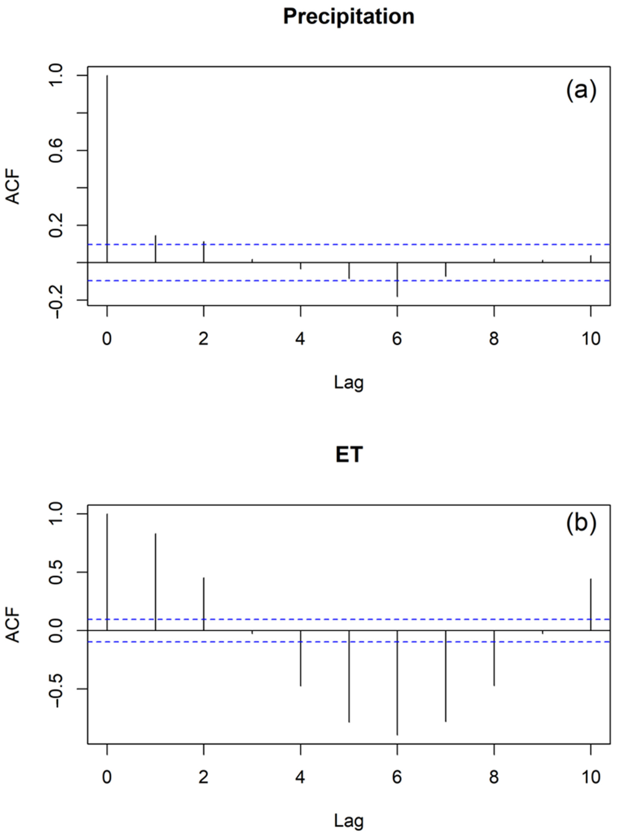
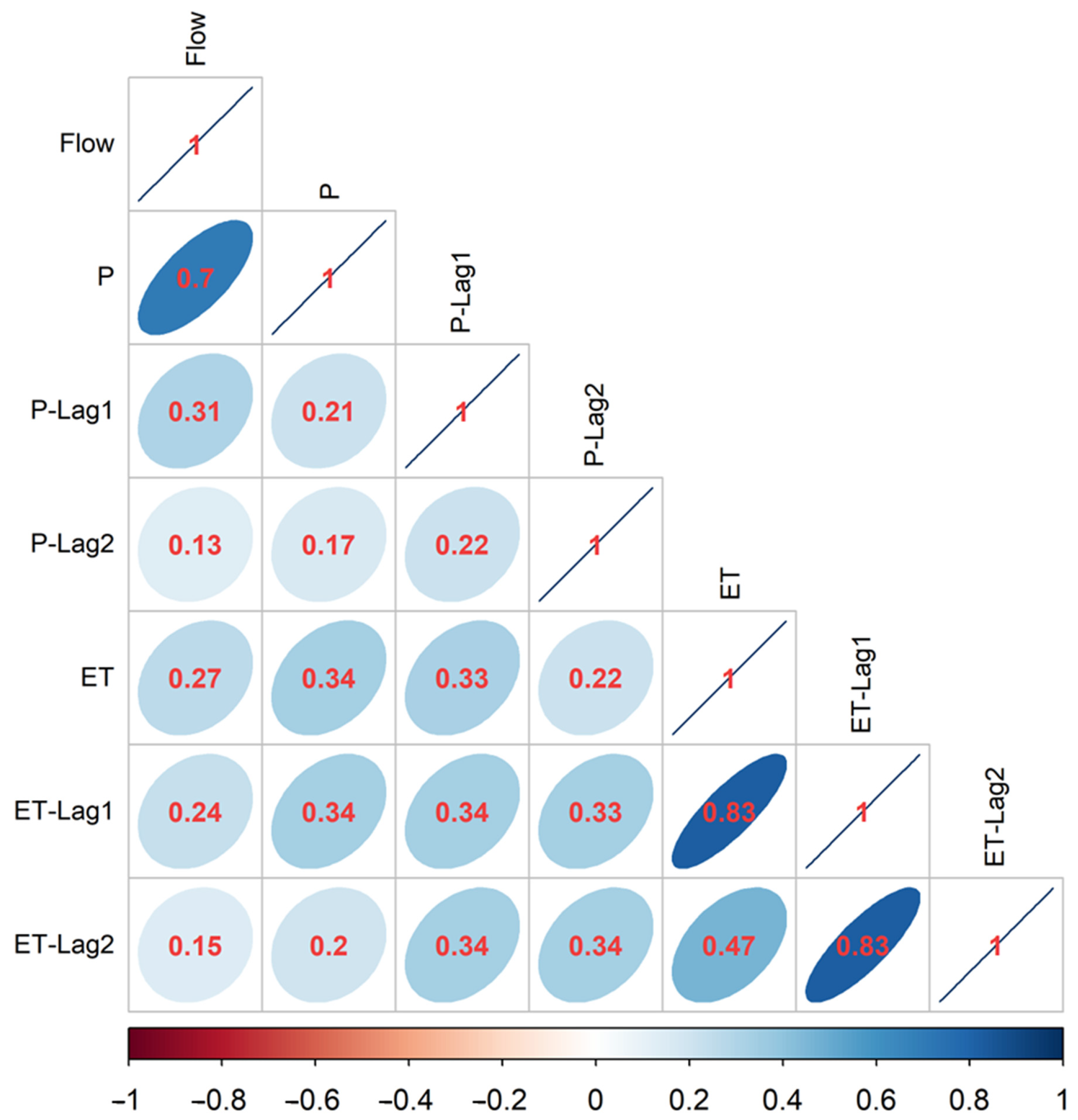
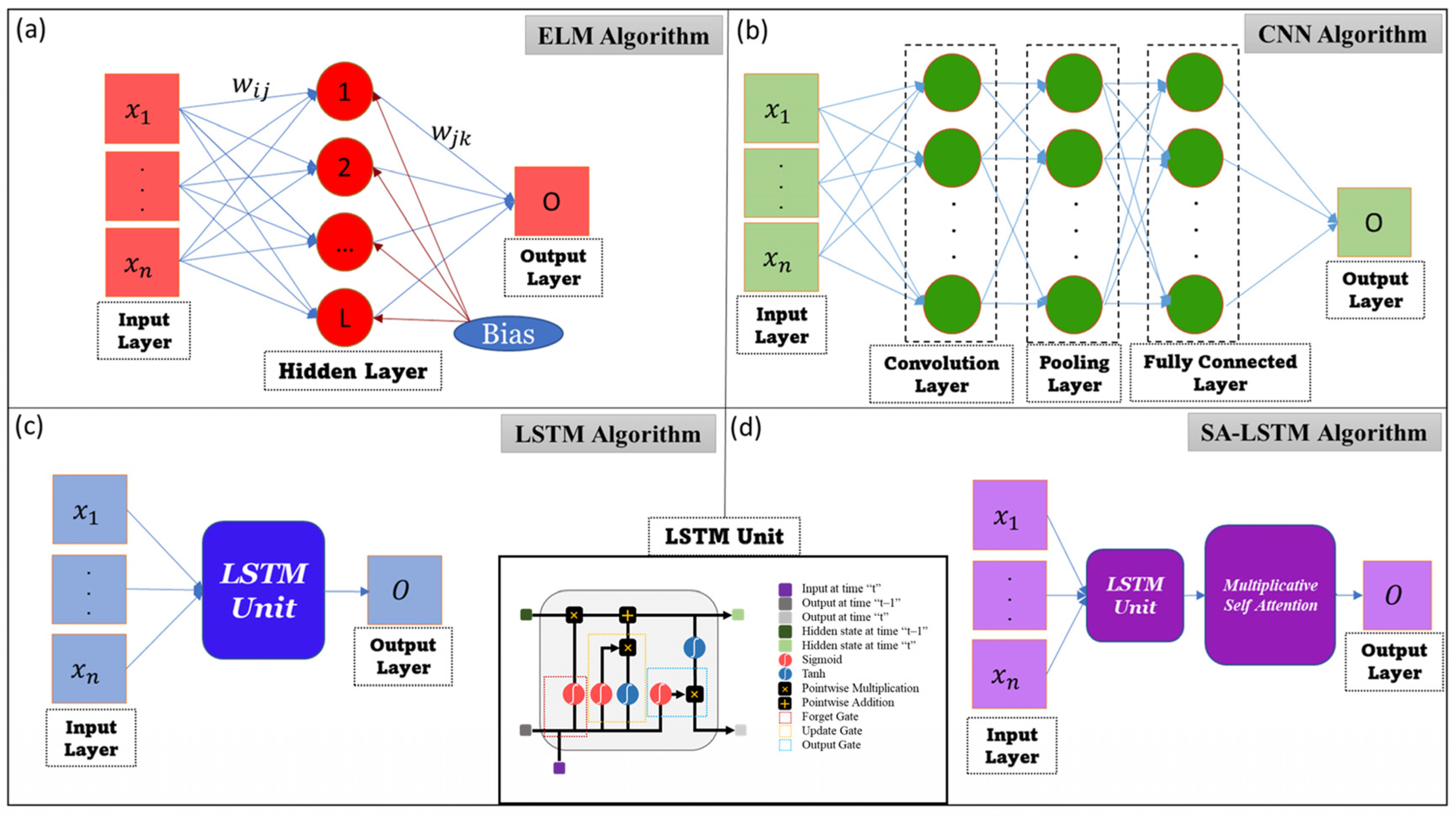
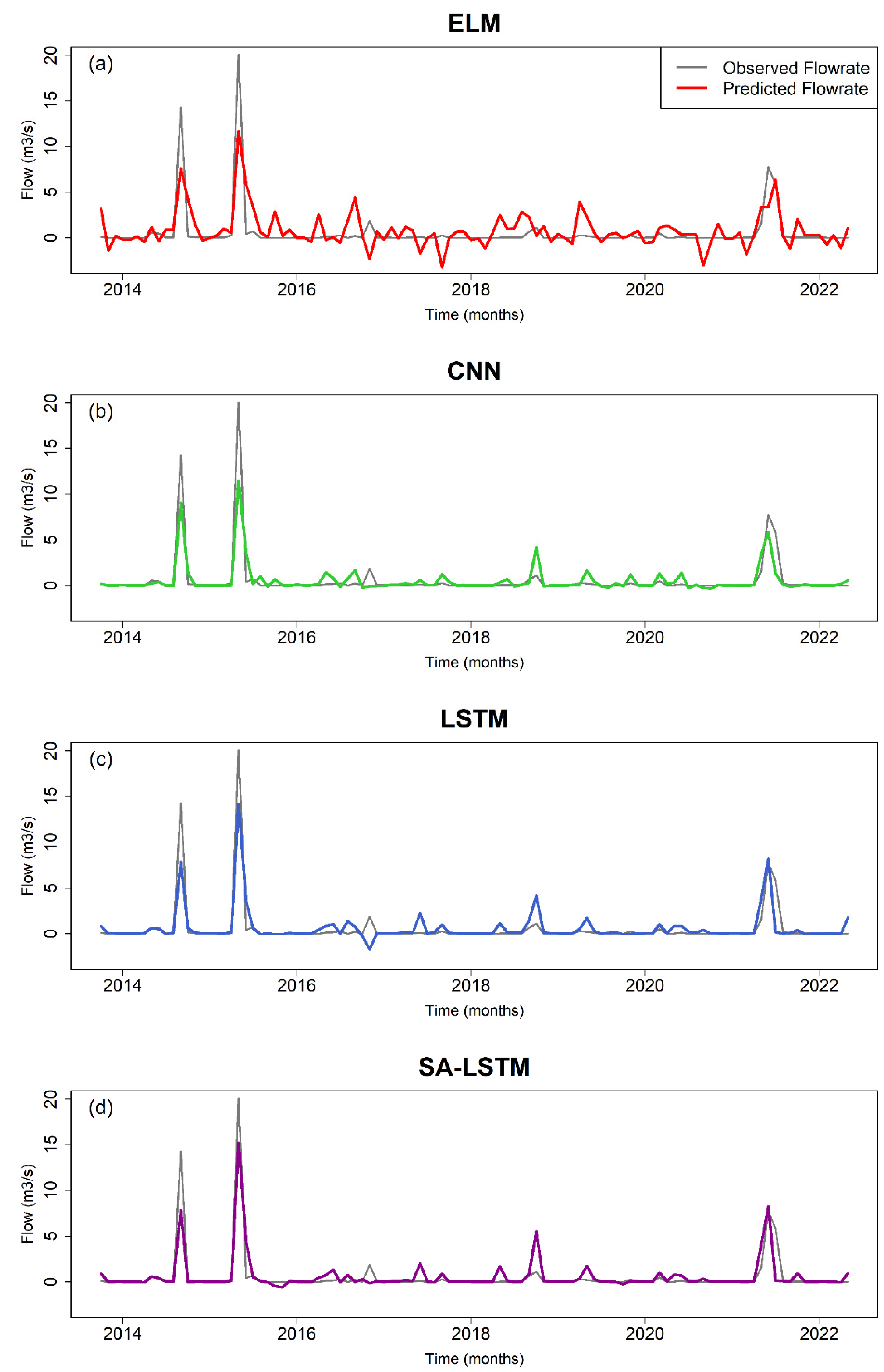
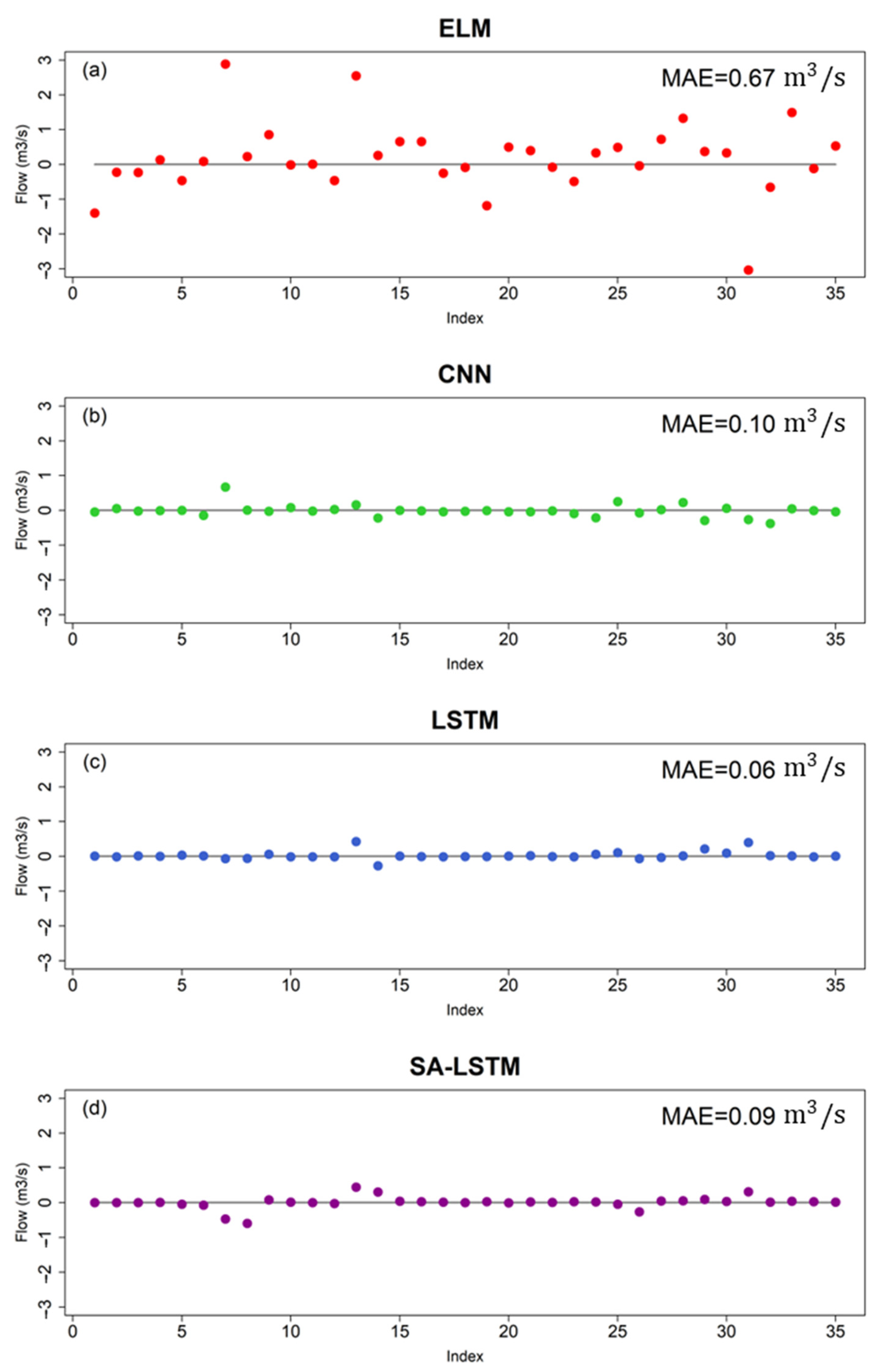
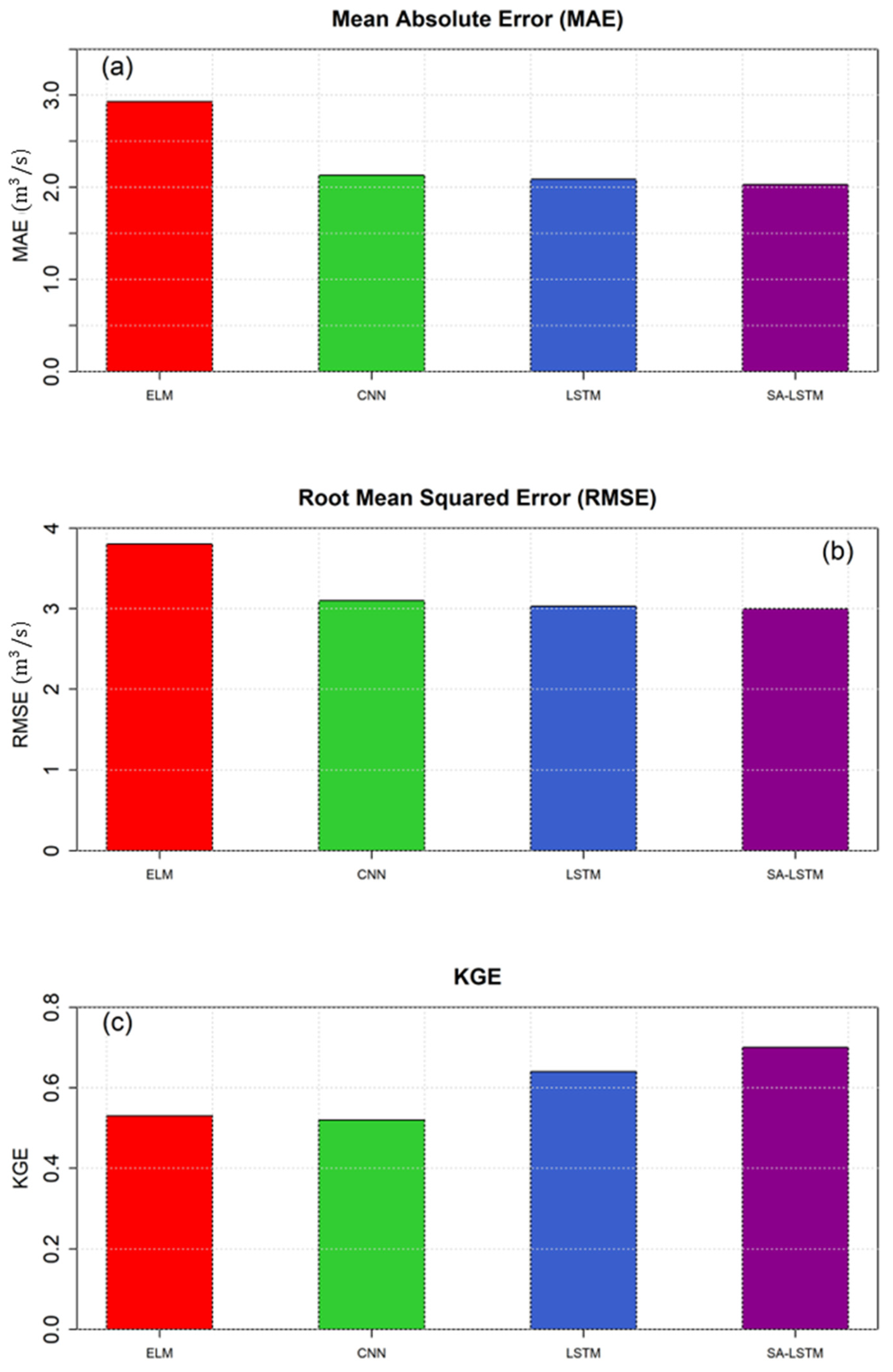
Table 1.
Summary of the hydro-meteorological data used for this study.
| Minimum | Median | Mean | Maximum | |
|---|---|---|---|---|
| Flowrate (m3/s) | 0 | 0.013 | 0.377 | 20.102 |
| Precipitation (mm) | 0 | 29.8 | 42.0 | 251.2 |
| ET (mm) | 2.1 | 64.8 | 80.6 | 221.33 |
Table 2.
Summary of model evaluation metrics during the training period.
| ELM | CNN | LSTM | SA–LSTM | |
|---|---|---|---|---|
| MAE (m3/s) | 0 | 0.02 | 0.04 | 0.04 |
| RMSE (m3/s) | 0 | 0.04 | 0.07 | 0.07 |
| d | 1 | 1 | 1 | 1 |
| r | 1 | 1 | 1 | 1 |
| R2 | 1 | 1 | 0.99 | 0.99 |
| NSE | 1 | 1 | 0.99 | 0.99 |
| KGE | 1 | 0.98 | 0.99 | 0.99 |
Table 3.
Summary of model evaluation metrics during the testing period (the best performing model is highlighted with respect to each metric).
Table 3.
Summary of model evaluation metrics during the testing period (the best performing model is highlighted with respect to each metric).
| ELM | CNN | LSTM | SA–LSTM | |
|---|---|---|---|---|
| MAE (m3/s) | 1.15 | 0.51 | 0.49 | 0.47 |
| RMSE (m3/s) | 1.85 | 1.28 | 1.26 | 1.24 |
| d | 0.81 | 0.9 | 0.92 | 0.92 |
| r | 0.7 | 0.9 | 0.88 | 0.88 |
| R2 | 0.49 | 0.82 | 0.78 | 0.77 |
| NSE | 0.47 | 0.75 | 0.76 | 0.76 |
| KGE | 0.48 | 0.63 | 0.7 | 0.73 |
Table 4.
Summary of the percentage of negative flowrate estimations by each model during the testing period.
Table 4.
Summary of the percentage of negative flowrate estimations by each model during the testing period.
| ELM | CNN | LSTM | SA–LSTM | |
|---|---|---|---|---|
| % of negative flowrates | 36% | 45% | 30% | 21% |
Table 5.
Summary of estimation errors for each model for the three highest flowrates during the testing period.
Table 5.
Summary of estimation errors for each model for the three highest flowrates during the testing period.
| Error in Flood Estimation% | ELM | CNN | LSTM | SA–LSTM |
|---|---|---|---|---|
| September 2014 | −47% | −37% | −39% | −39% |
| May 2015 | −42% | −43% | −29% | −24% |
| June 2021 | −56% | −25% | +6% | +6% |
Publisher’s Note: MDPI stays neutral with regard to jurisdictional claims in published maps and institutional affiliations. |
© 2022 by the authors. Licensee MDPI, Basel, Switzerland. This article is an open access article distributed under the terms and conditions of the Creative Commons Attribution (CC BY) license (https://creativecommons.org/licenses/by/4.0/).
Share and Cite
MDPI and ACS Style
Forghanparast, F.; Mohammadi, G. Using Deep Learning Algorithms for Intermittent Streamflow Prediction in the Headwaters of the Colorado River, Texas. Water 2022, 14, 2972. https://doi.org/10.3390/w14192972
AMA Style
Forghanparast F, Mohammadi G. Using Deep Learning Algorithms for Intermittent Streamflow Prediction in the Headwaters of the Colorado River, Texas. Water. 2022; 14(19):2972. https://doi.org/10.3390/w14192972
Chicago/Turabian StyleForghanparast, Farhang, and Ghazal Mohammadi. 2022. "Using Deep Learning Algorithms for Intermittent Streamflow Prediction in the Headwaters of the Colorado River, Texas" Water 14, no. 19: 2972. https://doi.org/10.3390/w14192972
Note that from the first issue of 2016, this journal uses article numbers instead of page numbers. See further details here.