Elastoplastic Coupled Model of Saturated Soil Consolidation under Effective Stress

 , ,
, ,
Abstract
:1. Introduction
2. Governing Equations
2.1. Equilibrium Equations
2.2. Continuity Equations
2.3. Darcy’s Law
2.4. Boundary Conditions
- (a)
- Pore pressure conditions:
- (b)
- Applied stress to the surface:
- (c)
- Superficial water flow:
- (d)
- Water flow into the soil:
- (e)
- Displacements on the soil boundary:
3. Constitutive Equations
3.1. Phenomenological Case of the Solid in the Soil
3.2. Phenomenological Case of the Flow in the Soil
4. Numerical Examples and Results
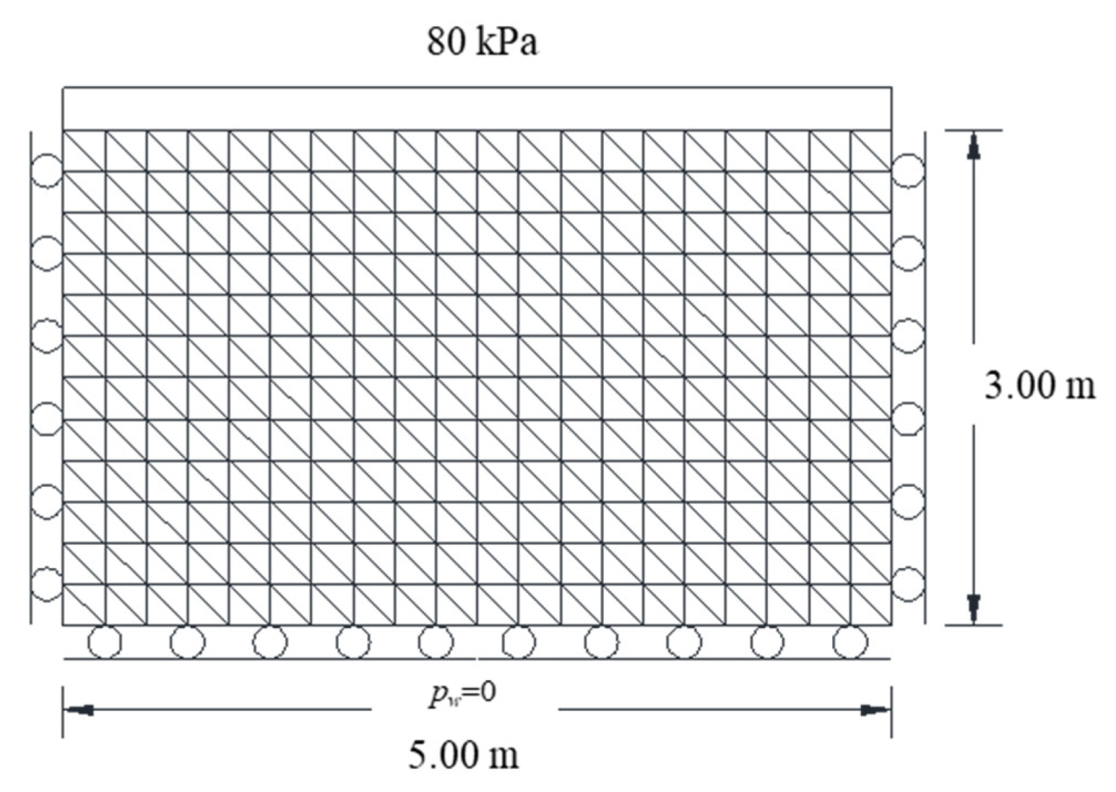
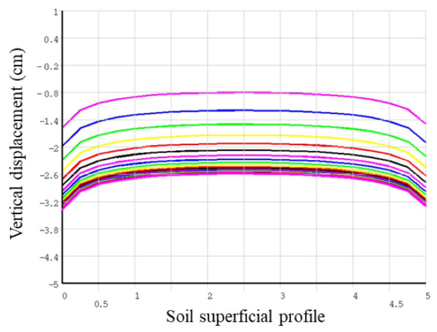
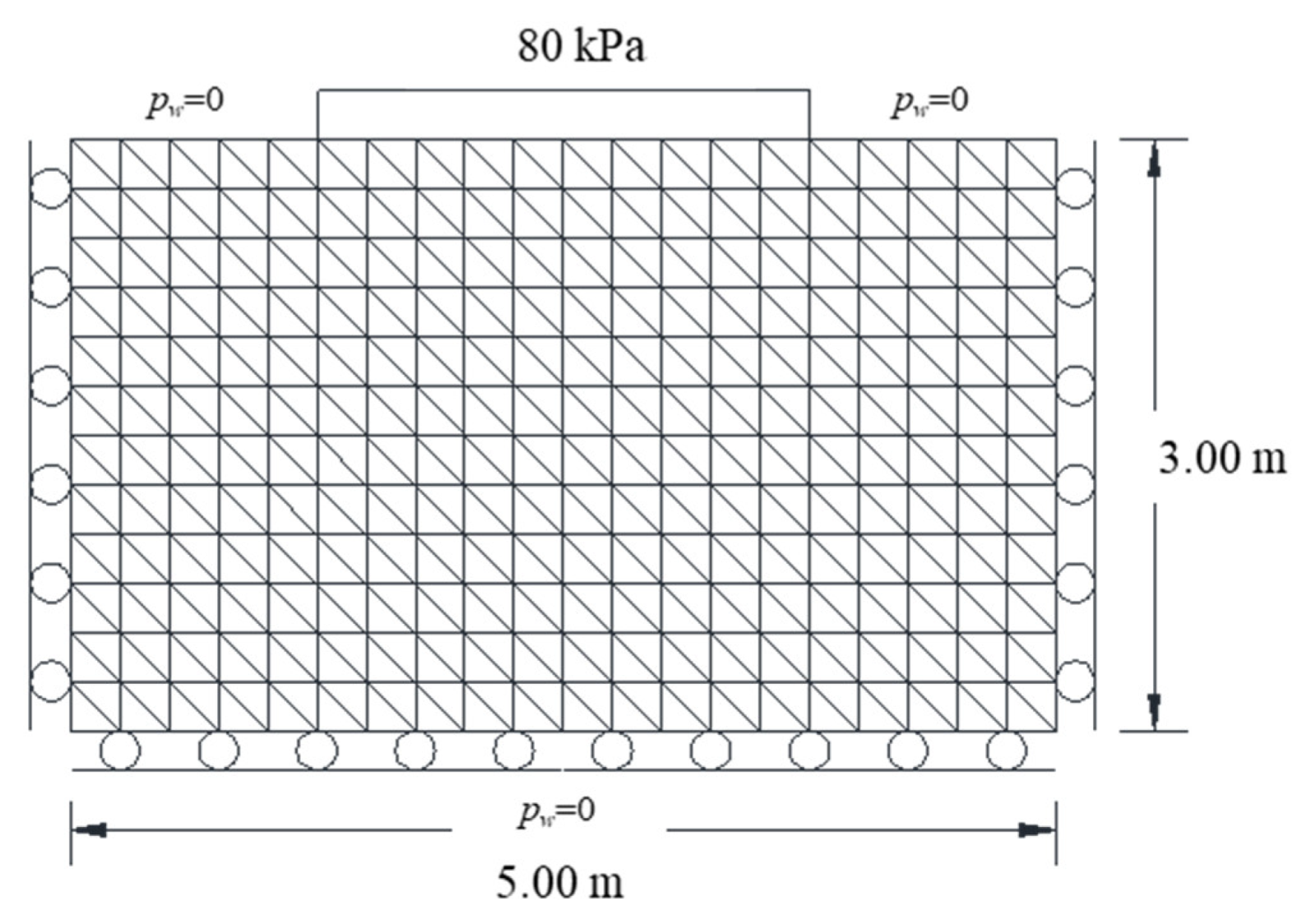
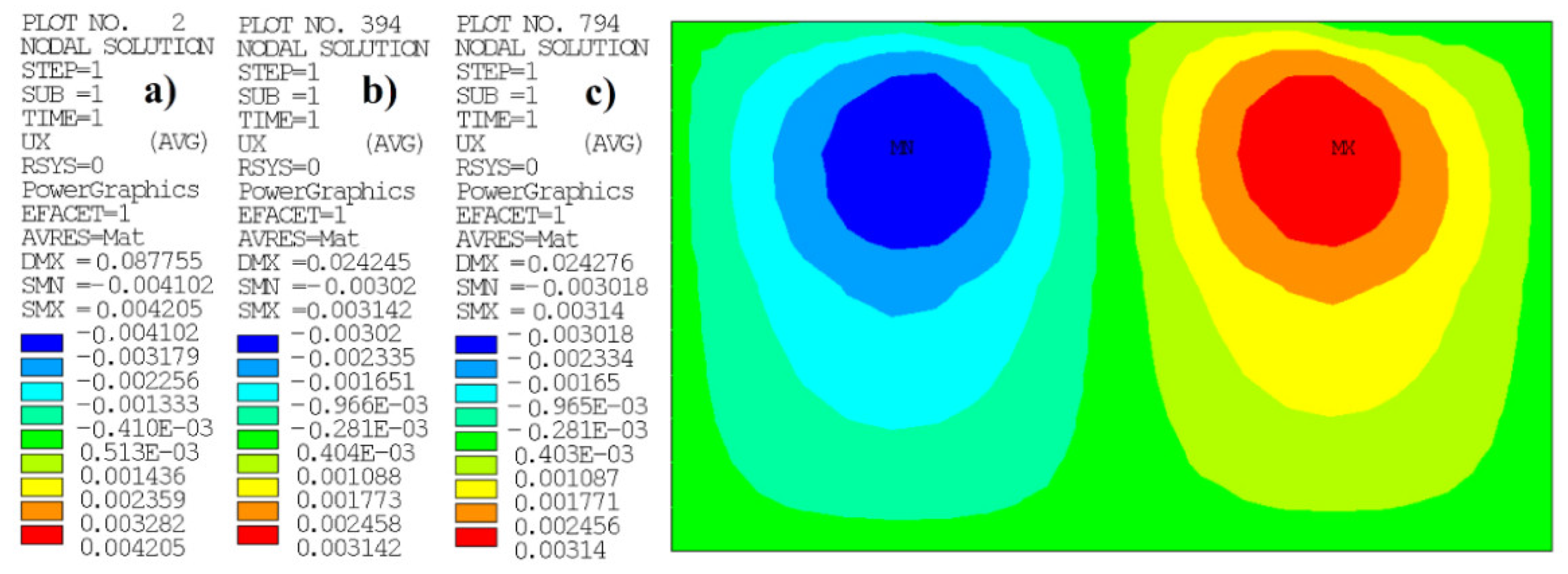
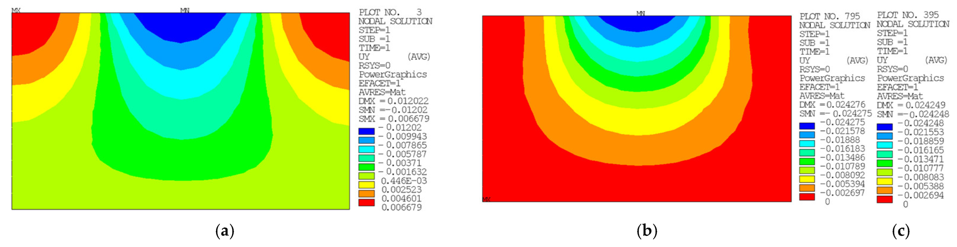
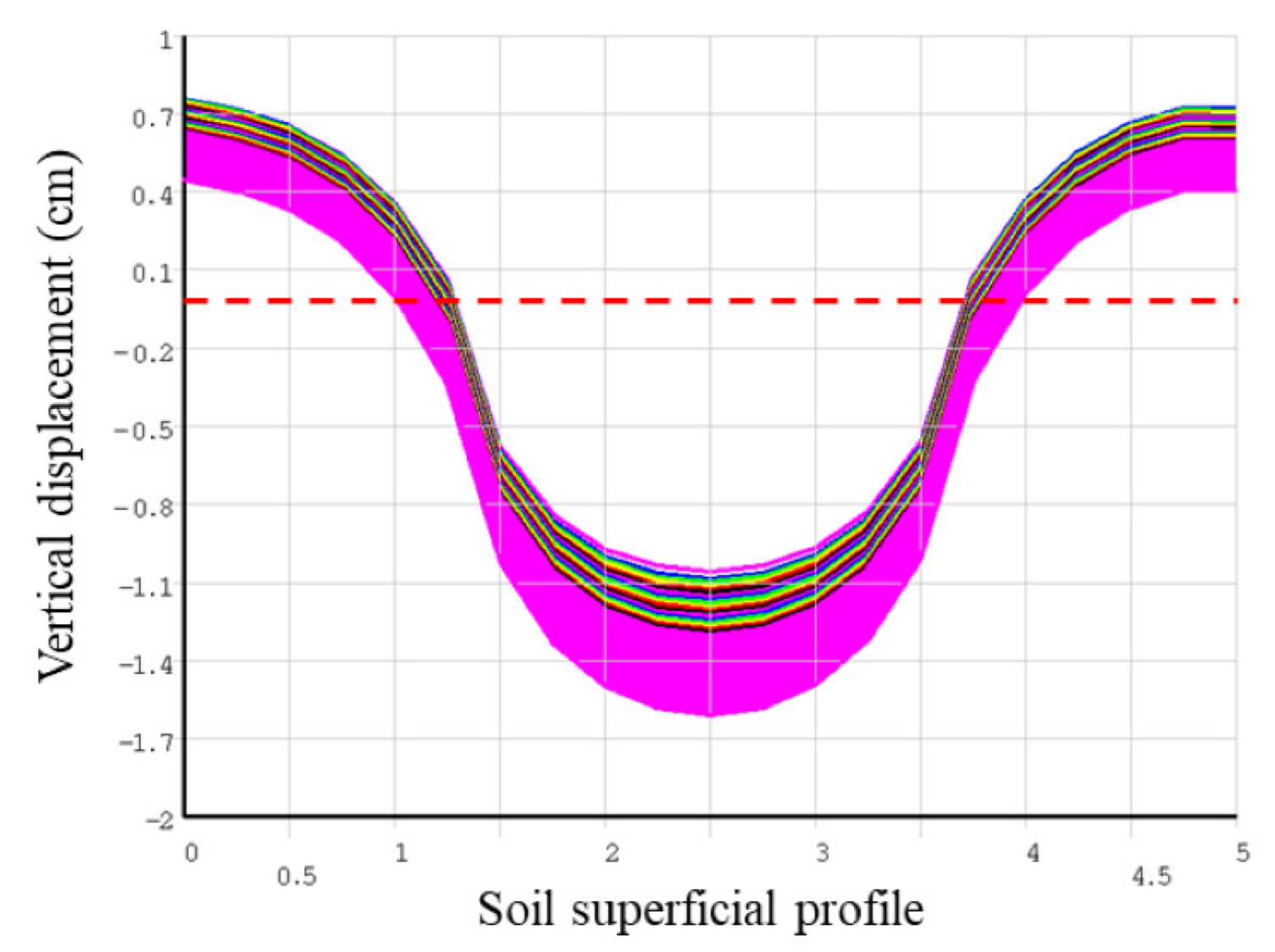
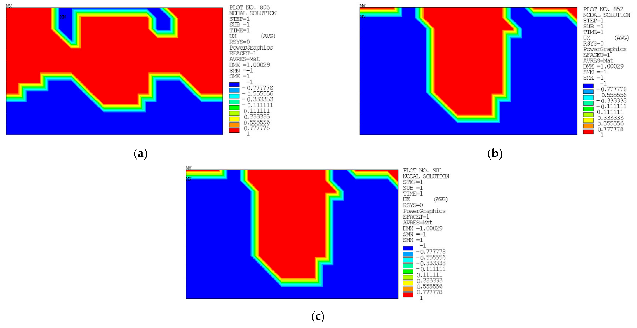
4.1. Case I: Vertical Flow (Bottom Boundary) under Lateral Restrictions
4.2. Case II: Vertical Flow (Top and Bottom Boundary) under Lateral Restrictions
5. Discussion
6. Conclusions
7. Future Work
Author Contributions
Funding
Institutional Review Board Statement
Informed Consent Statement
Data Availability Statement
Acknowledgments
Conflicts of Interest
Appendix A
Elastoplastic Coupled Model Formulation of the Soil Consolidation (Flow–Mechanical–Critical-State)


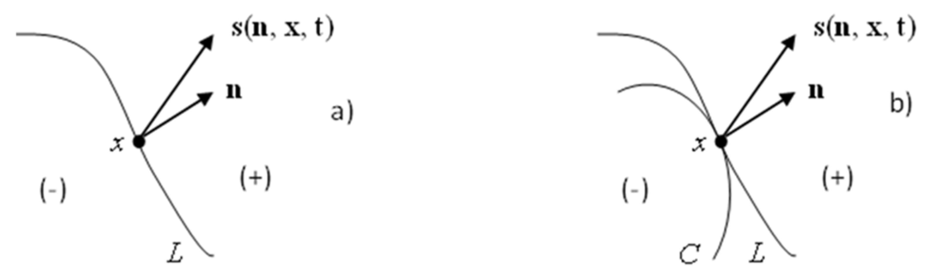
- (a)
- For each unit vector
- (b)
- The tensor is symmetric;
- (c)
- The tensor satisfies the motion equation:
Appendix B
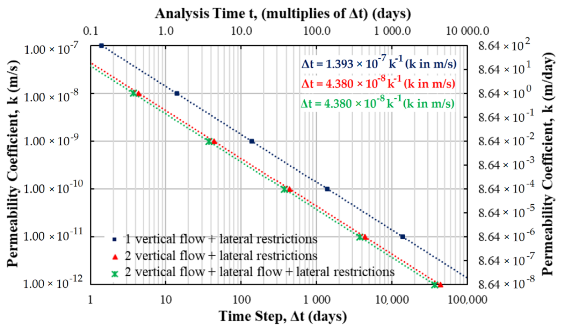
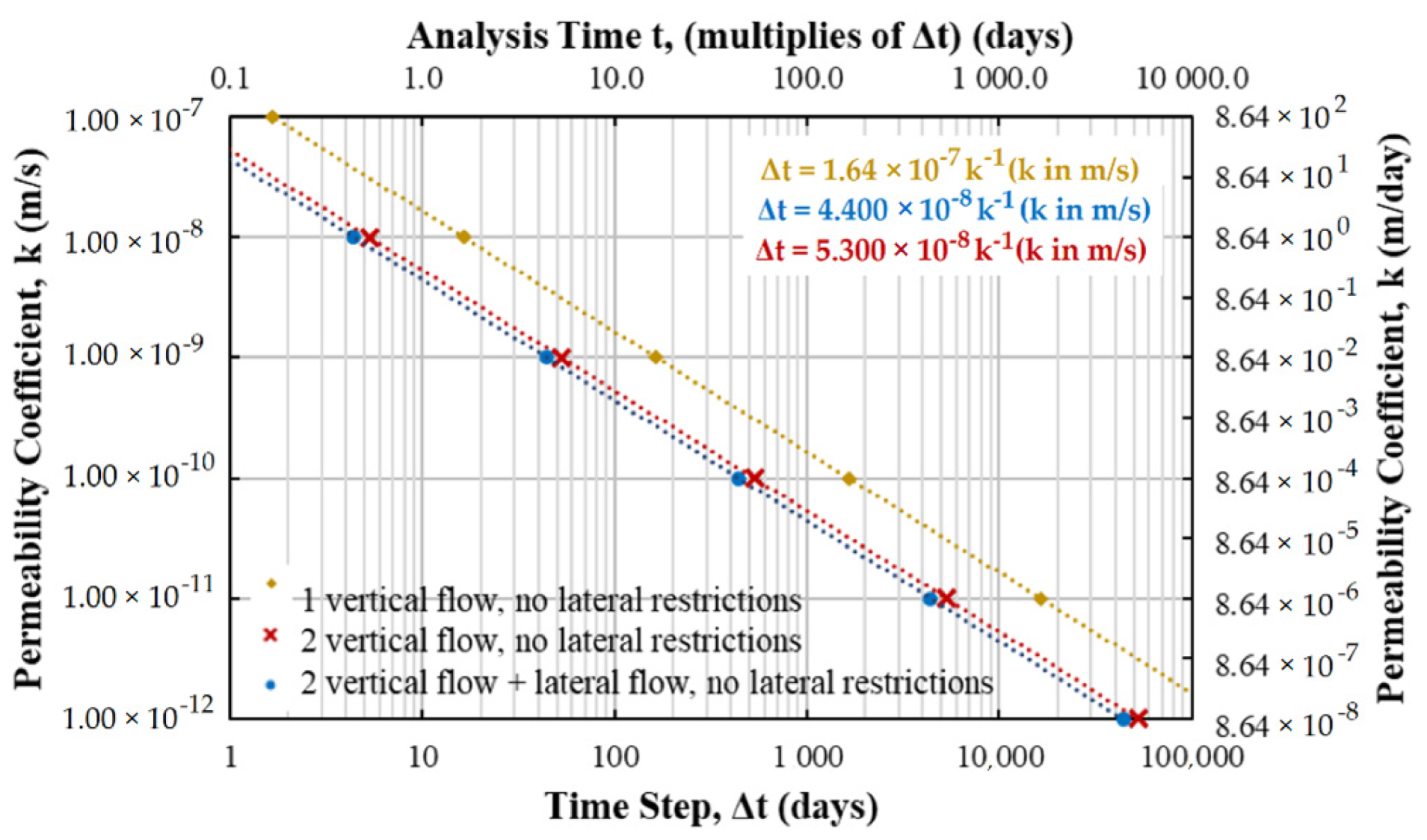
Calibration Curves of the Elastoplastic Coupled Model (Flow–Mechanical–Critical-State)


References
- Ahmad, A.; Sutanto, M.H.; Al-Bared, M.A.M.; Harahap, I.S.H.; Abad, S.V.A.N.K.; Khan, M.A. Physio-Chemical Properties, Consolidation, and Stabilization of Tropical Peat Soil Using Traditional Soil Additives—A State of the Art Literature Review. KSCE J. Civ. Eng. 2021, 25, 3662–3678. [Google Scholar] [CrossRef]
- Qi, S.; Simms, P.; Daliri, F.; Vanapalli, S. Coupling elasto-plastic behaviour of unsaturated soils with piecewise linear large-strain consolidation. Géotechnique 2020, 70, 518–537. [Google Scholar] [CrossRef]
- Xu, Z.; Cao, W.; Cui, P.; Li, H.; Wei, Y. Analysis of One-Dimensional Consolidation Considering Non-Darcian Flow Described by Non-Newtonian Index Incorporating Impeded Drainage Boundaries. Water 2022, 14, 1740. [Google Scholar] [CrossRef]
- Zhou, W.-H.; Zhao, L.-S. One-Dimensional Consolidation of Unsaturated Soil Subjected to Time-Dependent Loading with Various Initial and Boundary Conditions. Int. J. Geomech. 2014, 14, 291–301. [Google Scholar] [CrossRef]
- Ossa, A.; Lerma, C.; Flores, M.; Gaxiola, A. Effect of consolidation on the resilient response of soft soils in Mexico City. Case Stud. Constr. Mater. 2022, 16, e00888. [Google Scholar] [CrossRef]
- Radhika, B.P.; Krishnamoorthy, A.; Rao, A.U. A review on consolidation theories and its application. Int. J. Geotech. Eng. 2020, 14, 9–15. [Google Scholar] [CrossRef]
- Conte, E. Consolidation analysis for unsaturated soils. Can. Geotech. J. 2004, 41, 599–612. [Google Scholar] [CrossRef]
- Darkshanamurthy, V.; Fredlund, D.G.; Rahardjo, H. Coupled Three-dimensional Consolidation Theory of Unsaturated Porous Media. In Proceedings of the Fifth International Conference on Expansive Soils 1984: Preprints of Papers, Barton, Australia, 1 January 1984; pp. 99–103. [Google Scholar]
- Dong, Y.; Lu, N.; Fox Patrick, J. Drying-Induced Consolidation in Soil. J. Geotech. Geoenvironmental Eng. 2020, 146, 04020092. [Google Scholar] [CrossRef]
- Ho, L.; Fatahi, B.; Khabbaz, H. Analytical solution for one-dimensional consolidation of unsaturated soils using eigenfunction expansion method. Int. J. Numer. Anal. Methods Geomech. 2014, 38, 1058–1077. [Google Scholar] [CrossRef]
- Ho, L.; Fatahi, B.; Khabbaz, H. Analytical solution to axisymmetric consolidation in unsaturated soils with linearly depth-dependent initial conditions. Comput. Geotech. 2016, 74, 102–121. [Google Scholar] [CrossRef]
- Shan, Z.; Ling, D.; Ding, H. Exact solutions for one-dimensional consolidation of single-layer unsaturated soil. Int. J. Numer. Anal. Methods Geomech. 2012, 36, 708–722. [Google Scholar] [CrossRef]
- Wan-Huan, Z.; Shuai, T. Unsaturated Consolidation in a Sand Drain Foundation by Differential Quadrature Method. Procedia Earth Planet. Sci. 2012, 5, 52–57. [Google Scholar] [CrossRef]
- Ali, M.M. Identifying and Analyzing Problematic Soils. Geotech. Geol. Eng. 2011, 29, 343–350. [Google Scholar] [CrossRef]
- Al-Shamrani, M.A.; Dhowian, A.W. Experimental study of lateral restraint effects on the potential heave of expansive soils. Eng. Geol. 2003, 69, 63–81. [Google Scholar] [CrossRef]
- Puppala, A.J.; Manosuthikij, T.; Chittoori, B.C.S. Swell and shrinkage characterizations of unsaturated expansive clays from Texas. Eng. Geol. 2013, 164, 187–194. [Google Scholar] [CrossRef]
- Jones, L.D.; Jefferson, I. Expansive soils. In ICE Manual of Geotechnical Engineering; Burland, J., Ed.; ICE Publishing: London, UK, 2012; Volume I, pp. 413–441. [Google Scholar]
- Wang, L.; Sun, J.; Zhang, M.; Yang, L.; Li, L.; Yan, J. Properties and numerical simulation for self-weight consolidation of the dredged material. Eur. J. Environ. Civ. Eng. 2020, 24, 949–964. [Google Scholar] [CrossRef]
- Zhou, W.-H.; Zhao, L.-S.; Li, X.-B. A simple analytical solution to one-dimensional consolidation for unsaturated soils. Int. J. Numer. Anal. Methods Geomech. 2014, 38, 794–810. [Google Scholar] [CrossRef]
- Arroyo, H.; Rojas, E.; de la Luz Pérez-Rea, M.; Horta, J.; Arroyo, J. A porous model to simulate the evolution of the soil–water characteristic curve with volumetric strains. Comptes Rendus Mécanique 2015, 343, 264–274. [Google Scholar] [CrossRef]
- Qin, A.-f.; Chen, G.-j.; Tan, Y.-w.; Sun, D.-a. Analytical solution to one-dimensional consolidation in unsaturated soils. Appl. Math. Mech. 2008, 29, 1329–1340. [Google Scholar] [CrossRef]
- Wang, L.; Zhou, A.; Xu, Y.; Xia, X. Consolidation of partially saturated ground improved by impervious column inclusion: Governing equations and semi-analytical solutions. J. Rock Mech. Geotech. Eng. 2022, 14, 837–850. [Google Scholar] [CrossRef]
- Tang, C.-S.; Cheng, Q.; Gong, X.; Shi, B.; Inyang, H.I. Investigation on microstructure evolution of clayey soils: A review focusing on wetting/drying process. J. Rock Mech. Geotech. Eng. 2022. [Google Scholar] [CrossRef]
- Barman, D.; Dash, S.K. Stabilization of expansive soils using chemical additives: A review. J. Rock Mech. Geotech. Eng. 2022, 14, 1319–1342. [Google Scholar] [CrossRef]
- Chakraborty, S. Numerical Modeling for Long Term Performance of Soil-Bentonite Cut-Off Walls in Unsaturated Soil Zone. Master’s Thesis, Louisiana State University, Baton Rouge, LA, USA, 2009. [Google Scholar]
- Wu, H.; Cheng, S.; Li, Z.; Ke, G.; Liu, H. Study on Soil Water Infiltration Process and Model Applicability of Check Dams. Water 2022, 14, 1814. [Google Scholar] [CrossRef]
- Shaker, A.A.; Dafalla, M.; Al-Mahbashi, A.M.; Al-Shamrani, M.A. Predicting Hydraulic Conductivity for Flexible Wall Conditions Using Rigid Wall Permeameter. Water 2022, 14, 286. [Google Scholar] [CrossRef]
- Yang, G.; Xu, Y.; Huo, L.; Wang, H.; Guo, D. Analysis of Temperature Effect on Saturated Hydraulic Conductivity of the Chinese Loess. Water 2022, 14, 1327. [Google Scholar] [CrossRef]
- Bondì, C.; Castellini, M.; Iovino, M. Compost Amendment Impact on Soil Physical Quality Estimated from Hysteretic Water Retention Curve. Water 2022, 14, 1002. [Google Scholar] [CrossRef]
- Eyo, E.U.; Ng’ambi, S.; Abbey, S.J. An overview of soil–water characteristic curves of stabilised soils and their influential factors. J. King Saud Univ.—Eng. Sci. 2022, 34, 31–45. [Google Scholar] [CrossRef]
- Mady, A.Y.; Shein, E.V. Assessment of pore space changes during drying and wetting cycles in hysteresis of soil water retention curve in Russia using X-ray computed tomography. Geoderma Reg. 2020, 21, e00259. [Google Scholar] [CrossRef]
- Lu, N.; Likos, W.J.; Knovel. Unsaturated Soil Mechanics; Wiley: New York, NY, USA, 2004. [Google Scholar]
- Chen, G.; Wang, F.-T.; Li, D.-Q.; Liu, Y. Dyadic wavelet analysis of bender element signals in determining shear wave velocity. Can. Geotech. J. 2020, 57, 2027–2030. [Google Scholar] [CrossRef]
- Arroyo, H.; Rojas, E. Fully coupled hydromechanical model for compacted soils. Comptes Rendus Mécanique 2019, 347, 1–18. [Google Scholar] [CrossRef]
- Nuth, M.; Laloui, L. Advances in modelling hysteretic water retention curve in deformable soils. Comput. Geotech. 2008, 35, 835–844. [Google Scholar] [CrossRef]
- Oh, S.; Park, K.H.; Kwon, O.K.; Chung, W.J.; Shin, K.J. On the Hypothesis of Effective Stress in Consolidation and Strength for Unsaturated Soils. Appl. Mech. Mater. 2013, 256–259, 108–111. [Google Scholar] [CrossRef]
- Rojas, E. Resistencia Al Esfuerzo Cortante de Los Suelos No Saturados; Editorial Academica Espanola: Madrid, Spain, 2011. [Google Scholar]
- Tsiampousi, A.; Smith, P.G.C.; Potts, D.M. Coupled consolidation in unsaturated soils: From a conceptual model to applications in boundary value problems. Comput. Geotech. 2017, 84, 256–277. [Google Scholar] [CrossRef]
- Giraldo Zapata, V.M.; Botero Jaramillo, E.; Ossa Lopez, A. Implementation of a model of elastoviscoplastic consolidation behavior in Flac 3D. Comput. Geotech. 2018, 98, 132–143. [Google Scholar] [CrossRef]
- Fox, P.J.; Berles, J.D. CS2: A piecewise-linear model for large strain consolidation. Int. J. Numer. Anal. Methods Geomech. 1997, 21, 453–475. [Google Scholar] [CrossRef]
- Gibson, R.E.; England, G.L.; Hussey, M.J.L. The Theory of One-Dimensional Consolidation of Saturated Clays. Géotechnique 1967, 17, 261–273. [Google Scholar] [CrossRef]
- Fox Patrick, J.; Pu, H.-F.; Berles James, D. CS3: Large Strain Consolidation Model for Layered Soils. J. Geotech. Geoenvironmental Eng. 2014, 140, 04014041. [Google Scholar] [CrossRef]
- Fox, P.J. CS4: A large strain consolidation model for accreting soil layers. In Proceedings of the Geotechnics of High Water Content Materials Memphis, Tennessee, TN, USA, 28–29 January 1999; pp. 29–47. [Google Scholar]
- Fox Patrick, J.; Di Nicola, M.; Quigley Donald, W. Piecewise-Linear Model for Large Strain Radial Consolidation. J. Geotech. Geoenviron. Eng. 2003, 129, 940–950. [Google Scholar] [CrossRef]
- Pu, H.-F.; Fox, P.J.; Liu, Y. Model for large strain consolidation under constant rate of strain. Int. J. Numer. Anal. Methods Geomech. 2013, 37, 1574–1590. [Google Scholar] [CrossRef]
- Wissa Anwar, E.Z.; Christian John, T.; Davis Edward, H.; Heiberg, S. Consolidation at Constant Rate of Strain. J. Soil Mech. Found. Div. 1971, 97, 1393–1413. [Google Scholar] [CrossRef]
- Brandenberg Scott, J. iConsol.js: JavaScript Implicit Finite-Difference Code for Nonlinear Consolidation and Secondary Compression. Int. J. Geomech. 2016, 17, 04016149. [Google Scholar] [CrossRef]
- Fox Patrick, J. Coupled Large Strain Consolidation and Solute Transport. II: Model Verification and Simulation Results. J. Geotech. Geoenvironmental Eng. 2007, 133, 16–29. [Google Scholar] [CrossRef]
- Indraratna, B.; Zhong, R.; Fox Patrick, J.; Rujikiatkamjorn, C. Large-Strain Vacuum-Assisted Consolidation with Non-Darcian Radial Flow Incorporating Varying Permeability and Compressibility. J. Geotech. Geoenviron. Eng. 2017, 143, 04016088. [Google Scholar] [CrossRef]
- Wang, L.; Zhou, A.; Xu, Y.; Xia, X. One-dimensional consolidation of unsaturated soils considering self-weight: Semi-analytical solutions. Soils Found. 2021, 61, 1543–1554. [Google Scholar] [CrossRef]
- Blight, G.E. Strength and Consolidation Characteristics of Compacted Soils; Imperial College London: London, UK, 1961. [Google Scholar]
- Liakopoulos, A.C. Darcy’s coefficient of permeability as symmetric tensor of second rank. Int. Assoc. Sci. Hydrol. Bull. 1965, 10, 41–48. [Google Scholar] [CrossRef]
- Fredlund, D.G.; Hasan, J.U. One-dimensional consolidation theory: Unsaturated soils. Can. Geotech. J. 1979, 16, 521–531. [Google Scholar] [CrossRef]
- Dakshanamurthy, V.; Fredlund, D. Moisture and air flow in an unsaturated soil. In Proceedings of the 4th International Conference on Expansive Soils, Denver, CO, USA, 16–18 June 1980; 1980; pp. 514–532. [Google Scholar]
- Arroyo, H.; Rojas, E.; Arroyo, J. An effective stress approach for hydro-mechanical coupling of unsaturated soils. In Proceedings of the 3rd European Conference on Unsaturated Soils—“E-UNSAT 2016”, Web of Conferences, Paris, France, 12–14 September 2016; p. 17006. [Google Scholar]
- Oka, F.; Yashima, A.; Tateishi, A.; Taguchi, Y.; Yamashita, A. A cyclic elasto-plastic constitutive model for sand considering a plastic-strain dependence of the shear modulus. Géotechnique 1999, 49, 661–680. [Google Scholar] [CrossRef]
- Guo, G.; Fall, M. Advances in modelling of hydro-mechanical processes in gas migration within saturated bentonite: A state-of-art review. Eng. Geol. 2021, 287, 106123. [Google Scholar] [CrossRef]
- Bentler, D.J. Finite Element Analysis of Deep Excavations. Ph.D. Thesis, Virginia Polytechnic Institute and State University, Blacksburg, VA, USA, 1998. [Google Scholar]
- Di Rado, H.; Beneyto, P.; Mroginski, J.; Manzolillo, J.; Awruch, A. Análisis Tridimensional De La Consolidación De Suelos Saturados Utilizando El Mef. Mecánica Comput. 2004, 607–618. [Google Scholar]
- Krishnamoorthy, A. Consolidation analysis using finite element method. In Proceedings of the 12th International Conference of International Association for Computer Methods and Advances in Geomechanics (IACMAG), Goa, India, 1–6 October 2008; pp. 1157–1161. [Google Scholar]
- Manzolillo, J.E.; Di Rado, H.A.; Awruch, A.M. Simulación numérica del comportamiento de suelos saturados bajo cargas de fundaciones. In Proceedings of the Reunión de Comunicaciones Científicas y Tecnológicas, Resistencia, Argentina, 9–10 July 2000; pp. 1–4. [Google Scholar]
- Duncan, J.M.; Chang, C.-Y. Nonlinear Analysis of Stress and Strain in Soils. J. Soil Mech. Found. Div. 1970, 96, 1629–1653. [Google Scholar] [CrossRef]
- Gurtin, M.E. An Introduction to Continuum Mechanics; Academic Press: Cambridge, MA, USA, 1982. [Google Scholar]
- Wong, T.T.; Fredlund, D.G.; Krahn, J. A numerical study of coupled consolidation in unsaturated soils. Can. Geotech. J. 1998, 35, 926–937. [Google Scholar] [CrossRef]
- Georgiev, S.G. Variational Calculus on Time Scales; Nova Science Publishers: New York, NY, USA, 2018. [Google Scholar]
- Wood, D.M. Soil Behaviour and Critical State Soil Mechanics; Cambridge University Press: New York, NY, USA, 1990. [Google Scholar]
- Castro Barco, D.A. Terraplén de Prueba Sobre Suelos Blandos. Estudio del Campo de Desplazamientos. Civil Engineering. Bachelor’s Thesis, Universidad de Sevilla, Sevilla, Spain, 2017. [Google Scholar]
- Segerlind, L.J. Applied Finite Element Analysis; John Wiley & Sons: New York, NY, USA, 1991. [Google Scholar]


| Soil Property | Symbol | Magnitude |
|---|---|---|
| Elastic modulus | 20,000 kPa 2000 Ton/m2 | |
| Poisson’s ratio | 0.35 | |
| Coefficient of permeability (x direction) | 1.184 × 10⁻⁴ m/day 1.37 × 10⁻⁹ m/s | |
| Coefficient of permeability (y direction) | 1.184 × 10⁻⁴ m/day 1.37 × 10⁻⁹ m/s | |
| Preconsolidation stress | −120.0 kPa −12.0 Ton/m2 | |
| Internal friction angle | 30° | |
| Lambda | 0.20 | |
| Kappa | 0.02 | |
| Time for analysis | 1379.07 days | |
| Time step | 13.93 days |
| Soil Property | Symbol | Magnitude |
|---|---|---|
| Elastic modulus | 20,000 kPa 2000 Ton/m2 | |
| Poisson’s ratio | 0.35 | |
| Coefficient of permeability (x direction) | 1.184 × 10⁻⁴ m/day 1.37 × 10⁻⁹ m/s | |
| Coefficient of permeability (y direction) | 1.184 × 10⁻⁴ m/day 1.37 × 10⁻⁹ m/s | |
| Preconsolidation stress | −120.0 kPa −12.0 Ton/m2 | |
| Internal friction angle | 30° | |
| Lambda | 0.20 | |
| Kappa | 0.02 | |
| Time for analysis | 877 days | |
| Time step | 4.385 days |
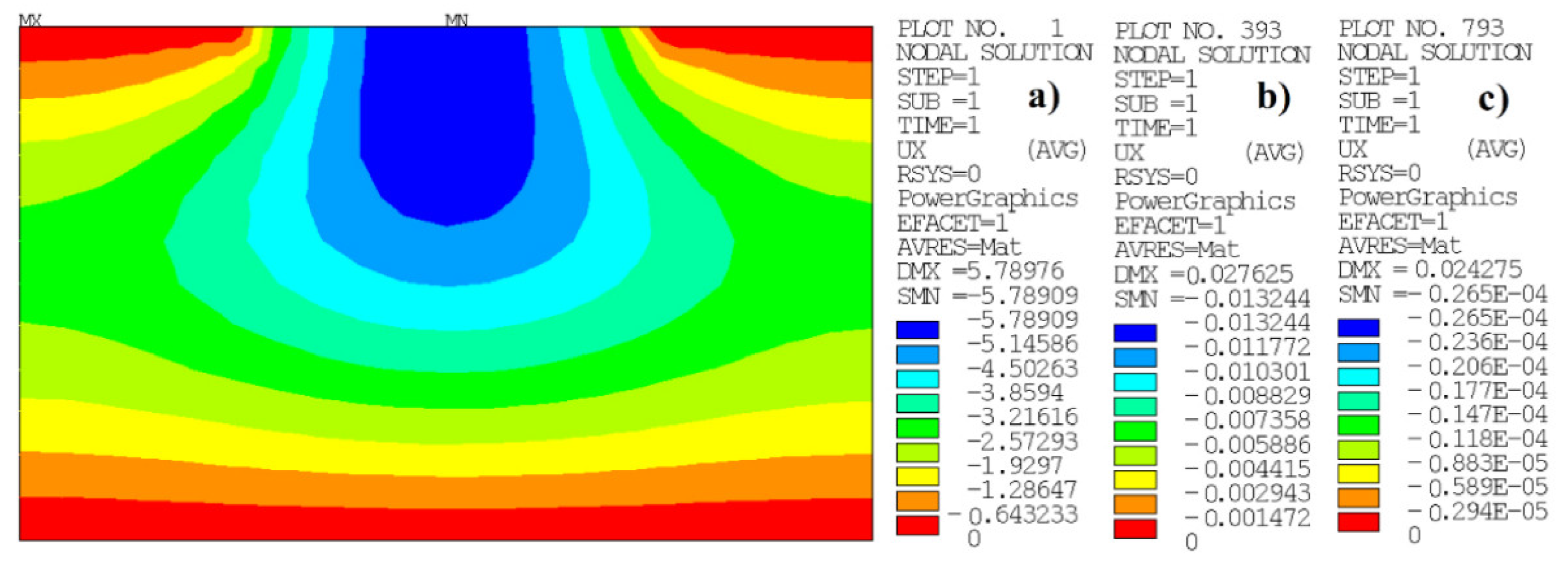
| With Superficial Flow | Without Superficial Flow | ||||
|---|---|---|---|---|---|
| Time Step | Water Pore Pressure | Time Step | Water Pore Pressure | ||
| (Days) | (kPa) | (Ton/m2) | (Days) | (kPa) | (Ton/m2) |
| 4.385 | −57.89 | −5.789090 | 13.93 | −79.87 | −7.987030 |
| 434.115 | −0.132 | −0.013244 | 682.57 | −0.219 | −0.021974 |
| 872.615 | −0.000 | −0.000027 | 1379.07 | −0.000 | −0.000046 |
Publisher’s Note: MDPI stays neutral with regard to jurisdictional claims in published maps and institutional affiliations. |
© 2022 by the authors. Licensee MDPI, Basel, Switzerland. This article is an open access article distributed under the terms and conditions of the Creative Commons Attribution (CC BY) license (https://creativecommons.org/licenses/by/4.0/).
Share and Cite
Galaviz-González, J.R.; Horta-Rangel, J.; Limón-Covarrubias, P.; Avalos-Cueva, D.; Cabello-Suárez, L.Y.; López-Lara, T.; Hernández-Zaragoza, J.B. Elastoplastic Coupled Model of Saturated Soil Consolidation under Effective Stress. Water 2022, 14, 2958. https://doi.org/10.3390/w14192958
Galaviz-González JR, Horta-Rangel J, Limón-Covarrubias P, Avalos-Cueva D, Cabello-Suárez LY, López-Lara T, Hernández-Zaragoza JB. Elastoplastic Coupled Model of Saturated Soil Consolidation under Effective Stress. Water. 2022; 14(19):2958. https://doi.org/10.3390/w14192958
Chicago/Turabian StyleGalaviz-González, José Roberto, Jaime Horta-Rangel, Pedro Limón-Covarrubias, David Avalos-Cueva, Laura Yessenia Cabello-Suárez, Teresa López-Lara, and Juan Bosco Hernández-Zaragoza. 2022. "Elastoplastic Coupled Model of Saturated Soil Consolidation under Effective Stress" Water 14, no. 19: 2958. https://doi.org/10.3390/w14192958