A Novel GRA-NARX Model for Water Level Prediction of Pumping Stations

Abstract

It is necessary but difficult to accurately predict the water levels in front of the pumping stations of an open-channel water transfer project because of the complex interactions among hydraulic structures. In this study, a novel GRA-NARX (gray relation analysis—nonlinear auto-regressive exogenous) model is proposed based on a gray relation analysis (GRA) and nonlinear auto-regressive exogenous (NARX) neural network for 2 h ahead for the prediction of water levels in front of pumping stations, in which an improved algorithm of the NARX neural network is used to obtain the optimal combination of the time delay and the hidden neurons number, and GRA is used to reduce the prediction complexity and improve the prediction accuracy by filtering input factors. Then, the sensitivity to changes of the training algorithm is analyzed, and the prediction performance is compared with that of the NARX and GRA-BP (gray relation analysis back-propagation) models. A case study is performed in the Tundian pumping station of the Miyun project, China, to demonstrate the reliability and accuracy of the proposed model. It is revealed that the GRA-NARX-BR (gray relation analysis—nonlinear auto-regressive exogenous—Bayesian regularization) model has higher accuracy than the model based only on a NARX neural network and the GRA-BP model with a correlation coefficient (R) of 0.9856 and a mean absolute error (MAE) of 0.00984 m. The proposed model is effective in predicting the water levels in front of the pumping stations of a complex open-channel water transfer project.

1. Introduction

Large-scale water transfer projects contribute significantly to mitigating the uneven distribution of water resources in a country. In an open-channel water transfer project consisting of a wide variety of hydraulic structures for different purposes, the water level between two adjacent pumping stations should be kept as constant as possible to avoid possible channel overflow or drying-up of the pumping station forebay. A sharp change in water level may cause water supply disruption and substantial hydraulic oscillation [1]. For this reason, an accurate prediction of water levels in front of pumping stations is of vital importance for the normal operation of these pumping stations.

The water levels of open-channel water transfer projects, natural lakes, or rivers are usually predicted using physically based models or machine learning models. The physically based models are mainly based on hydrodynamic models with Saint Venant equations as the governing equations to simulate one-dimensional channel flow, and the use of these models is somewhat limited because they require complete information about the study area [2,3]. Machine learning models mainly include the relevance vector machine (RVM) model [4], grey model(1,1) (GM (1,1)) model [5], multiple linear regression model [6], and neural network model [7,8,9,10,11,12,13,14,15,16,17,18,19,20]. The first three models are applicable to complex prediction situations, but their prediction accuracy is not sufficiently high. In contrast, neural network models are increasingly used for water-level prediction in recent years. The back-propagation (BP) neural network has a strong nonlinear fitting ability but has no feedback memory nodes [13,14,15]. The long short-term memory (LSTM) network has several memory blocks consisting of an output gate, an input gate, a forget gate, and a memory cell, and it is effective for volatile time series [21]. The Elman neural network (ENN) has a high capacity for learning any dynamic input–output relationship. However, it substitutes less trustworthy learning for streamlined derivative calculations [22]. The nonlinear auto-regressive exogenous (NARX) neural network is a recurrent dynamic network composed of input delay and feedback memory nodes, and it is widely used for complex multi-input and multi-output systems [23]. It also significantly outperforms other artificial neural network (ANN) methods in terms of how quickly it reaches the weights for connections between neurons and input parameters [24] and reduces the number of the parameters to build an efficient model [25]. Previous studies about the NARX models have focused more on extreme values in high-tide prediction, groundwater-level prediction, and drought and flood prediction. For example, Di Nunno et al. [26] established two different NARX-based models for extreme storm tide events that were both more accurate than existing models. Additionally, Di Nunno and Granata [27] discovered that the NARX neural network could precisely forecast the fluctuation of the daily groundwater levels of 76 wells located in Apulia, Italy. Wunsch et al. [28] found that the NARX neural network was stable for predicting groundwater levels of several wells in fractured, porous, and karst aquifers in southwest Germany for up to half a year. Ezzeldin and Hatata [29] revealed that the NARX neural network was better than all other models available in the literature for predicting the flow at the side orifice. Wang et al. [30] demonstrated that the NARX neural network could be successfully used to predict droughts and floods in the Yangtze River basin, China. Fan et al. [31] found that the NARX neural network was better than the BP neural network in predicting the nonlinear and cumulative characteristics of dam deformation time series.

The choice of input variables will have an impact on the prediction accuracy of the neural network model. The input factors should be filtered to reduce the prediction complexity and improve the prediction accuracy. Gray relational analysis (GRA) is a quantitative method to explore the dissimilarity and similarity among factors, and it has no strict requirement on the distribution and number of the dataset. In recent years, many prediction models have been proposed by combining GRA with neural networks. When predicting the fertilization of forests, Chen et al. [32] discovered that the gray relation analysis—particle swarm optimization—back-propagation (GRA-PSO-BP) model was more reliable than the BP and BP-PSO models. Chen and Lin [33] found that the GRA-LSTM model was robust in the short-term forecasting of PV power plants. Chen et al. [34] developed the GRA-NARX model to forecast changes of dissolved oxygen mass concentration in surface water; however, the model’s accuracy tends to decline with time.

It is worth noting that few GRA-NARX models are available for predicting water levels in front of pumping stations. Moreover, in previous NARX models, the time delay and the hidden neurons number are selected based on experience [35,36], and there is a need to determine the optimal combination of the time delay and the hidden neurons number to obtain the most accurate prediction. In addition, Levenberg–Marquardt (LM) is the most frequently used training algorithm in current NARX neural networks and other algorithms are seldom used. The primary goal of this study is to investigate the reliability and accuracy of the novel GRA-NARX model for the water-level prediction of a pumping station forebay in an open-channel water transfer project, as well as the sensitivity to changes in the training algorithm. Our major contributions are threefold:

• A novel water-level prediction model is proposed based on gray relation analysis (GRA) and NARX neural network with the optimal combination of the time delay and the hidden neurons number for prediction of water levels in front of the pumping stations of a water transfer project.
• The sensitivity to changes of the training algorithm is analyzed.
• The case study is performed in the Tundian pumping station of the Miyun project, China, and the results show that our model outperforms the NARX and GRA-BP models.

The remainder of this paper is structured as follows. Section 2 describes the study area and methods used in this work. The experimental results are presented in Section 3. The discussion is presented in Section 4. Section 5 contains the conclusions and recommendations for future work.

2. Study Area and Methods

2.1. Study Area

The Miyun project (Figure 1) was put into operation in May 2015 to supply water to Beijing, the capital city of China. The hydrodynamic characteristics, such as water levels in front of pumping stations, gate opening, and flow rates, were available under different operating and weather conditions. Six pumping stations (P1–P6) were built at the Tundian gate, Liulin inverted siphon, Jingtou inverted siphon, Xingshou inverted siphon, Lishishan control gate, and Xitai plunge control gate to pump water from the Jingmi water diversion canal to the Huairou Reservoir, and there is no storage reservoir along the route. Three pumping stations (P7–P9) were built from Guojiawu to Xiwongzhuang with a total length of 31 km, including 8 km of the original Jingmi water diversion canal, 22 km of single prestressed concrete cylinder pipe (PCCP) (2.6 m in diameter), and 800 m of steel pipeline. For the last three pressurized pumping stations, the flow rate is about 10 m³/s.

The Tundian pumping station located on the north side of the Tundian control gate of the Jingmi water diversion canal in Haidian District was selected for the case study. This pumping station is used in cooperation with the Tundian control gate for water lifting with a design head of 1.71 m. It is 8.1 km away from the upstream control node at the Tuancheng Lake north gate, and the main hydraulic structures along the route include the Anhe Yang gate, Nongda diversion gate, Donggan diversion gate, Beigan diversion gate, Huimin Cemetery Yanglui gate, Wuyi diversion gate, Hanjiachuan Yang gate, and Cuijiayao diversion gate. It is 9.5 km away from the downstream control node at the former Liulin pumping station, and the main hydraulic structures along the route include the Lengquan Bridge floodgate, Tai Zhouwu floodgate, Samsung Zhuang floodgate, Hot Spring inverted siphon, Bei’an River floodgate, and former Liulin inverted siphon. The water-flow conditions are rather complex, making it difficult for water-level prediction.

2.2. Methods

2.2.1. Cleaning and Interpolation of Water-Level Data

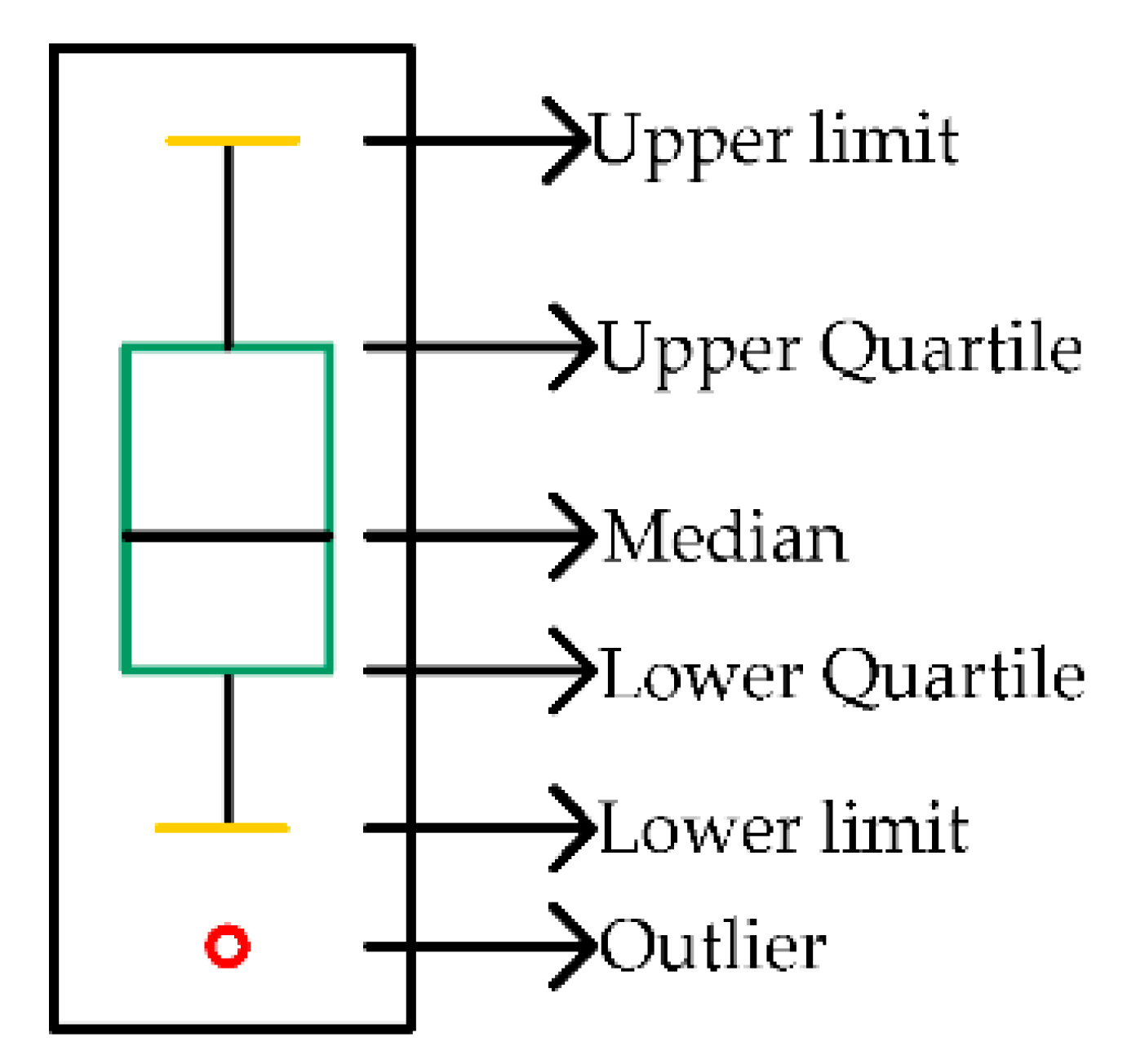
As outliers are frequently present in water-level data because of various factors, such as equipment failure, human activities, and climate change, the original water-level data needs to be cleaned to ensure the accuracy of the prediction. The box plot method is often used to detect possible outliers in a dataset, and, unlike the z-score method or the Grubbs method, it does not require the data to follow a normal distribution [37]. The box plot contains five statistical points: lower quartile $S_1$, median $S_2$, upper quartile $S_3$, lower limit, and upper limit. The distance between upper and lower quartiles is the inter-quartile distance IQR, and the upper and lower limit are expressed as $S_3+1.5IQR$ and $S_1-1.5IQR$, respectively, as shown in Figure 2. A value smaller than the lower limit or larger than the upper limit is identified as an outlier. Finally, all outliers are rejected and interpolated.

2.2.2. Selection of the Main Influencing Factors of Water-Level Information

The current water level in front of a pumping station can be influenced by a number of factors, such as the water level at the previous moment, or an earlier flow rate of the pumping station, or the flow-rate difference between the downstream and upstream of the pumping station. However, only the main influencing factors are considered to reduce the prediction complexity and improve the prediction accuracy. GRA is a statistical technique to explore the dissimilarity and similarity among influencing factors and it has no strict requirement on the number and distribution of the dataset. The specific steps are as follows:

Step 1: Determine the comparison and reference sequences. The current water level in front of the pumping station is taken as the reference sequence ($x_0=\{x_0(k)\left|k=1,2,3,\dots ,n\right.\}$), and the influencing factors are taken as the comparison sequences ($x_i=\{x_i(k)\left|k=1,2,3,\dots ,n\right.\}, i=1,2,3,\dots m$). There are m comparison sequences and n evaluation indexes.

Step 2: Dimensionless processing of comparison and reference sequences.

Step 3: Calculate the gray relational coefficient between reference and comparison sequences, which is defined as follows:

$${\xi }_i(k)=\frac{\underset{i}{\min }(\underset{k}{\min }\left|x_0(k)-x_i(k)\right|)+\rho \underset{i}{\max }(\underset{k}{\max }\left|x_0(k)-x_i(k)\right|)}{\left|x_0(k)-x_i(k)\right|+\rho \underset{i}{\max }(\underset{k}{\max }\left|x_0(k)-x_i(k)\right|)}$$

(1)

where $\rho$ is the resolution coefficient, which is in the range of $(0,1)$, and the larger the resolution coefficient, the larger the resolution will be. The best resolution is $\rho =0.5463$, and it is usually taken to be $\rho =0.5$.

Step 4: Calculate the gray relation between reference and comparison sequences:

$$r_i=\frac{1}{n}{\displaystyle \sum _{k=1}^n{\xi }_i}(k),i=1,2,3,\dots ,m$$

(2)

Step 5: Sort the gray relation according to the size. The closer the $r_i$ value is to 1, the higher the influence of the comparison sequence on the reference sequence will be. If the gray relation is less than 0.6, the two sequences are considered to be not correlated, while if the gray relation is greater than 0.8, the two sequences are considered to be highly correlated.

2.2.3. NARX Neural Network Model for Pumping Station Forebay

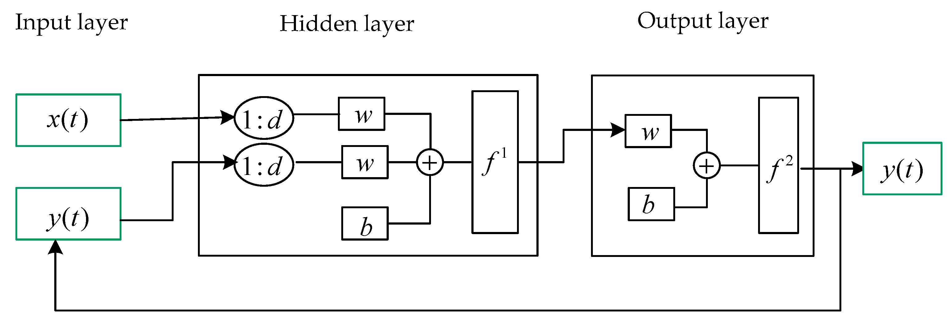
The NARX neural network is made up of interconnected nodes that stand in for synthetic neurons that receive one or more inputs and elaborate them to produce an output. These sums go through a nonlinear activation function. There are three layers in the network: the input, hidden, and output layers (Figure 3). The input layer contains the input parameters of the neural network, the hidden layer between input and output layers has several hidden neurons, the output layer gives the predicted value y(t), and then the output is fed back to the input. If one of the following conditions is fulfilled, the NARX process is terminated: the maximum number of epochs; the training algorithm adjustment parameter; or the error gradient below a minimal value. The NARX model is implemented in MATLAB^®2020.

The NARX model can be expressed as:

$$y(t)=f(x(t-1),x(t-2),\dots x(t-d),y(t-1),y(t-2),\dots y(t-d))$$

(3)

where f is a nonlinear function; x(t) is the input value representing the influencing factors of the current water level in front of the pumping station; y(t) is the output value representing the current water level in front of the pumping station; and d is the time delay evaluated by the optimal combination of the time delay and the hidden neurons number. y(t) can be obtained from the previous values of x(t) and y(t) by nonlinear mapping. The network inputs are $x_1,x_2,\dots ,x_n$, and the output of each layer is calculated as:

$$H_j=f({\displaystyle \sum _{i=1}^n{w}_{ij}}{x}_i-b_j)$$

(4)

where $w_{ij}$ is the weight; $b_j$ is the bias; and $f(f=f^{1}or$$f=f^2)$ is the activation function. The sigmoid activation function $f^1$ is used for the hidden layer, while the linear activation function $f^2$ with only one neuron, n, is used for the output layer. The weight $w_{ij}$ and bias $b_j$ of the NARX model are optimized based on the training algorithm. More details can be found in [38].

2.2.4. Training Algorithms

Three training algorithms including Levenberg–Marquardt (LM), Bayesian regularization (BR), and scaled conjugate gradient (SCG) are used and compared in this study. LM converges fast with a stable convergence rate and it is regularly employed for the time-series prediction of neural networks; BR performs well in difficult problems and is a Gauss–Newton approximation to the Hessian matrix; SCG is an iterative algorithm for large linear systems with a convergence speed between the first two of the inputs [10].

2.2.5. Evaluation Metrics

The correlation coefficient (R), mean square error (MSE), root mean square error (RMSE), and mean absolute error (MAE) are used to assess the performance of the GRA-NARX, NARX, and GRA-BP models. R denotes the relationship between the observed and predicted values and it is in the range of 0–1, where 1 denotes perfect agreement between the observed and predicted values and 0 denotes no relationship. RMSE, MSE, and MAE indicate the magnitude of the disparity between the predicted and observed values, and the smaller the RMSE, MSE, and MAE values are, the better the prediction will be.

$$MAE=\frac{{\displaystyle \sum _{i=1}^m\left|f_i-y_i\right|}}{m}$$

(5)

$$MSE=\frac{{\displaystyle \sum _{i=1}^m{(f_i-y_i)}^2}}{m}$$

(6)

$$R=\frac{\left|{\displaystyle \sum _{i=1}^m(y_i}-\overline{y_i})(f_i-\overline{f_i})\right|}{\sqrt{{({\displaystyle \sum _{i=1}^m{y}_i-\overline{y_i}})}^2{({\displaystyle \sum _{i=1}^m{f}_i-\overline{f_i}})}^2}}$$

(7)

$$RMSE=\sqrt{\frac{{\displaystyle \sum _{i=1}^m{(f_i-y_i)}^2}}{m}}$$

(8)

where m is the total number of observed data; $f_i$ is the predicted value of the $i$ th data; $y_i$ is the observed value of the $i$ th data; and $\overline{y_i}$ and $\overline{f_i}$ are the average of the observed data and the predicted data.

2.2.6. Evaluation of the Time Delay and the Hidden Neurons Number

In the existing literature, the selection of the time delay and the hidden neurons number is dependent entirely on the experience. To verify the accuracy of the GRA-NARX model, different MSE values are obtained under different combinations of the time delay and the hidden neurons number, and the minimal MSE indicates the optimal combination. The improved algorithm of the NARX model is shown in

Table 1. Improved algorithm of the NARX model.

Algorithm 1 NARX Model Improved Algorithm

1. nDelays = 1:n; 2. Hidden neurons = 1:m; 3. bestPerformance = 1; 4. bestDeylay = 0; 5. bestHidden neurons = 0; 6. performanceMap = zeros(length(nDelays), length(hidden neurons)); 7. for nd = 1:length(nDelays) 8.  nDelay = nDelays(nd); 9.  inputDelays = 1:nDelay; 10.  feedbackDelays = 1:nDelay; 11.  for hs = 1:length(hidden neurons) 12.   hidden neurons = hidden neurons(hs); 13.   net = narxnet(inputDelays, feedbackDelays, hidden neurons); 14. performanceMap(nd, hs) = performance; 15.   if performance < bestPerformance 16.    disp([‘best performance:’, num2str(performance)]); 17.    disp([‘bset delay:’, num2str(nDelay)]); 18.    disp([‘best hidden neurons: ’, num2str(hidden neurons)]); 19.    bestPerformance = performance; 20.    bestDeylay = nDelay; 21.    besthidden neurons = hidden neurons; 22.    bestNet = net; 23.   end 24.   end 25.  end

.

2.2.7. GRA-NARX Neural Network Model for Pumping Station Forebay

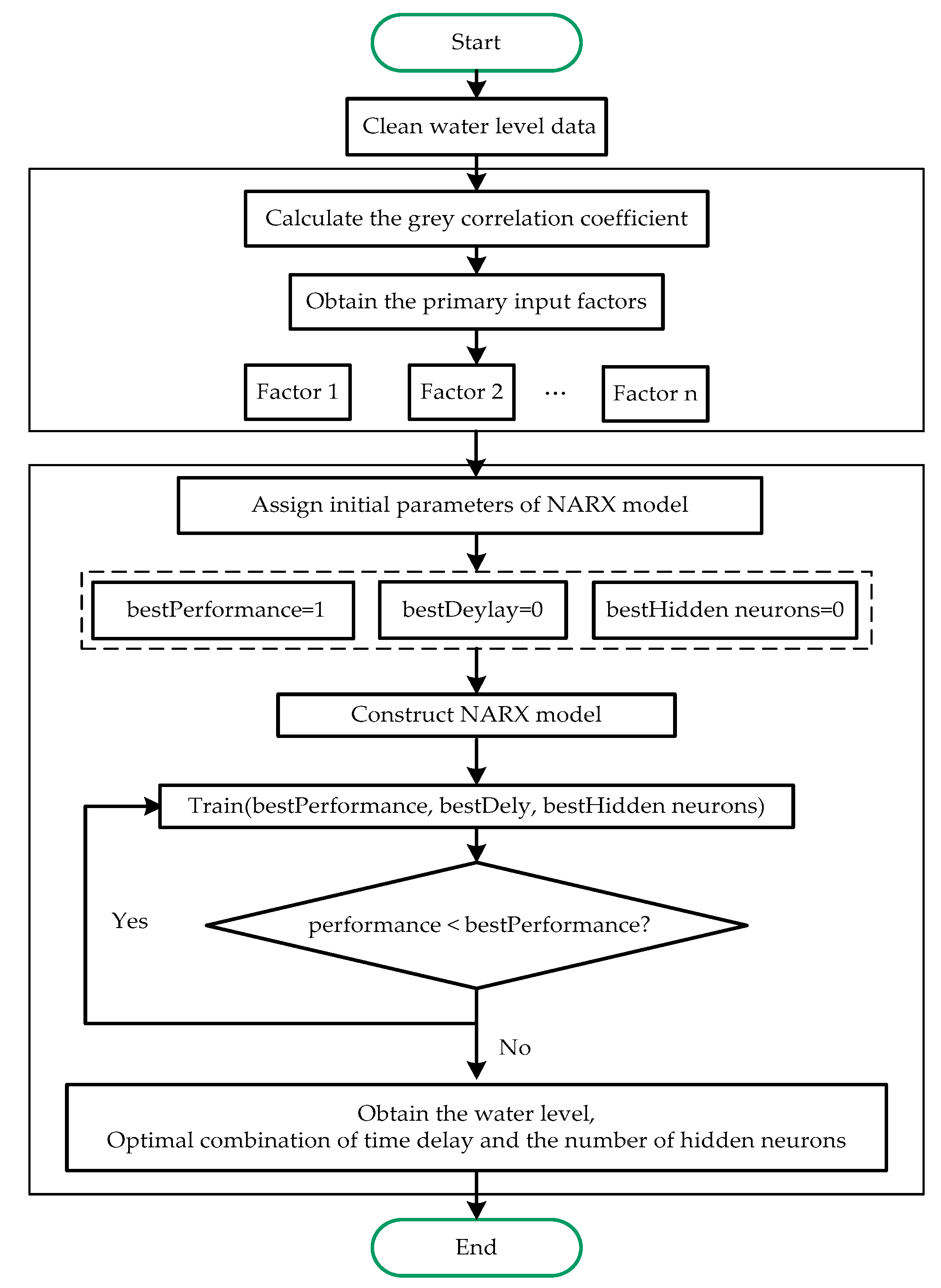
The GRA-NARX neural network model is constructed as follows. First, the water-level data is cleaned using the box plot method and interpolated using the mean fill method. Then, the main influencing factors of the current water level are identified by GRA and then input into the NARX neural network. The training algorithm, the time delay, and the number of neurons in the hidden layer are determined. The flowchart of the water-level prediction model based on the GRA-NARX neural network is shown in Figure 4.

3. Results

3.1. Cleaning of Water-Level Data

A total of 2868 water levels were recorded at intervals of 2 h in front of the Tundian pumping station from 11 March 2016 to 10 November 2016. The data were cleaned using the box plot method as described in Section 2.2.1, in which the upper quartile was 49.2, the lower quartile was 49.07, the upper limit was 49.395, and the lower limit was 48.875. The values higher than the upper limit and lower than the lower limit were identified as outliers. A total of 20 outliers were identified, as shown in

Table 2. Outliers in the monitoring data.

Time	Water Level/m	Time	Water Level/m
20 July 20:00:00	49.52	17 September 14:00:00	48.85
20 July 22:00:00	49.59	7 October 22:00:00	48.87
20 July 00:00:00	49.59	9 October 04:00:00	48.86
20 July 02:00:00	49.45	10 October 12:00:00	48.86
17 September 00:00:00	48.87	14 October 04:00:00	48.87
17 September 02:00:00	48.77	15 October 08:00:00	48.87
17 September 04:00:00	48.75	26 October 02:00:00	48.86
17 September 06:00:00	48.86	3 November 04:00:00	48.87
17 September 10:00:00	48.87	3 November 06:00:00	48.86
17 September 12:00:00	48.80	6 November 16:00:00	48.87

, and then these values and the original null values were interpolated using the mean fill method.

3.2. Selection of the Main Influencing Factors of Water-Level Information

The current water level in front of the pumping station may be affected by a wide variety of factors, mainly including the flow rate, water level before and after the pumping station, and water level of the last station before and after the gate at the previous moment. The current water level in front of the Tundian pumping station is used as the reference sequence, and the five influencing factors at the previous moment (two hours ago) are taken as the comparison sequences, where r₁ is the previous moment flow rate in front of the Tundian pumping station, r₂ is the previous moment water level in front of the Tundian pumping station, r₃ is the previous moment water level after the Tundian pumping station, r₄ is the previous moment water level in front of the end of Tuan Cheng Lake, and r₅ is the previous moment water level after Tuan Cheng Lake. The 2868 pieces of cleaned data were converted into dimensionless values to eliminate the difference in scale and unit, and the gray relational coefficients were calculated as described in Section 2.2.2. The gray correlation between each influencing factor and the current water level in front of the pumping station is shown in

Table 3. Grey correlation between each influencing factor and the current water level in front of the pumping station.

No.	Factor	Correlation
1	r1	0.6512
2	r2	0.9456
3	r3	0.8669
4	r4	0.6401
5	r5	0.6417

.

Therefore, the next-moment water level in front of the Tundian pumping station (two hours later) is predicted using r₂ and r₃ as the inputs of the neural network model and the current water level in front of the Tundian pumping station as the output of the GRA-NARX neural network model.

3.3. Construction of Prediction Model

3.3.1. GRA-NARX Model

Considering the GRA results, the previous-moment water levels in front of and after the Tundian pumping station were used as the input factors of the neural network model, and the current water level in front of the Tundian pumping station was used as the output factor. Then, the NARX neural network model was used to train and test the dataset. Respectively, 70%, 15%, and 15% of the 2868 pieces of water-level data were randomly selected for training, verification, and testing, according to experience and the trial-and-error method; “tansig” and “purelin” were the transfer functions of the hidden layer and the output layer, respectively. The maximum iteration number was 1000, the learning rate was 10⁻³, and the error gradient was 10⁻⁷. The range of the time delay and the hidden neurons number was 1–14 and 1–20, respectively, and their optimal combination was obtained as described in Section 2.2.6. Other parameters were set to default values.

3.3.2. GRA-BP Model

When using the same input, various neural networks can be compared for how they affect it. The input and output factors, the ratio of input data division, the number of neurons in the hidden layer, and the transfer functions of the hidden and output layers of the GRA-BP neural network were the same as those of the GRA-NARX neural network, but the output of the GRA-NARX neural network was fed back to the input at the next moment.

3.3.3. NARX Model

The input factors of the NARX model included the previous-moment flow of the Tundian pumping station, the previous-moment water level in front of the Tundian pumping station, the previous-moment water level after the Tundian pumping station, the previous-moment water level before the gate at the end of Tuancheng Lake, and the previous-moment water level after the gate at the end of Tuancheng Lake, and the output factor was the current water level in front of the Tundian pumping station. Other network training parameters were the same as those of the GRA-NARX neural network.

3.4. Results and Analysis of GRA-NARX Model

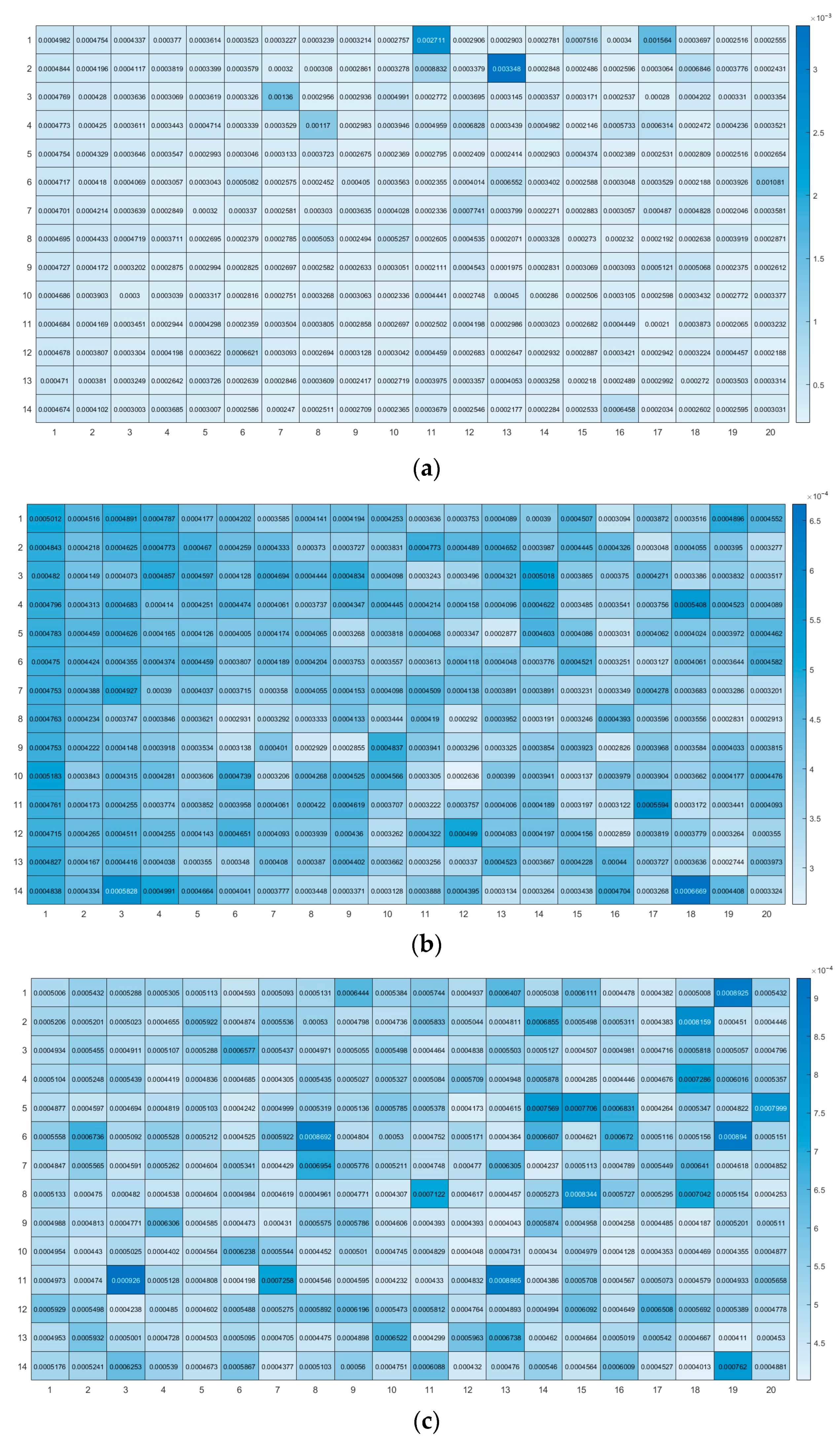
According to Section 2.2.6 and Section 3.3.1, the range of the time delay is set to 1–14 and that of the hidden neurons number is set to 1–20. The MSE values for the GRA-NARX model under different combinations of the time delay and the hidden neurons number are shown in Figure 5, where a lighter color indicates a smaller MSE value. Figure 5a reveals that when BR is used as the training algorithm, the MSE value reaches a minimum of 0.0001975 when the time delay is 9 and the hidden neurons number is 13. Figure 5b reveals that when LM is used as the training algorithm, the MSE value reaches a minimum of 0.0002636 when the time delay is 10 and the hidden neurons number is 12. Figure 5c reveals that when SCG is used as the training algorithm, the MSE value reaches a minimum of 0.0004013 when the time delay is 14 and the hidden neurons number is 18. Therefore, it is concluded that the use of BR as the training algorithm yields the best prediction results.

3.5. Comparison with Other Models

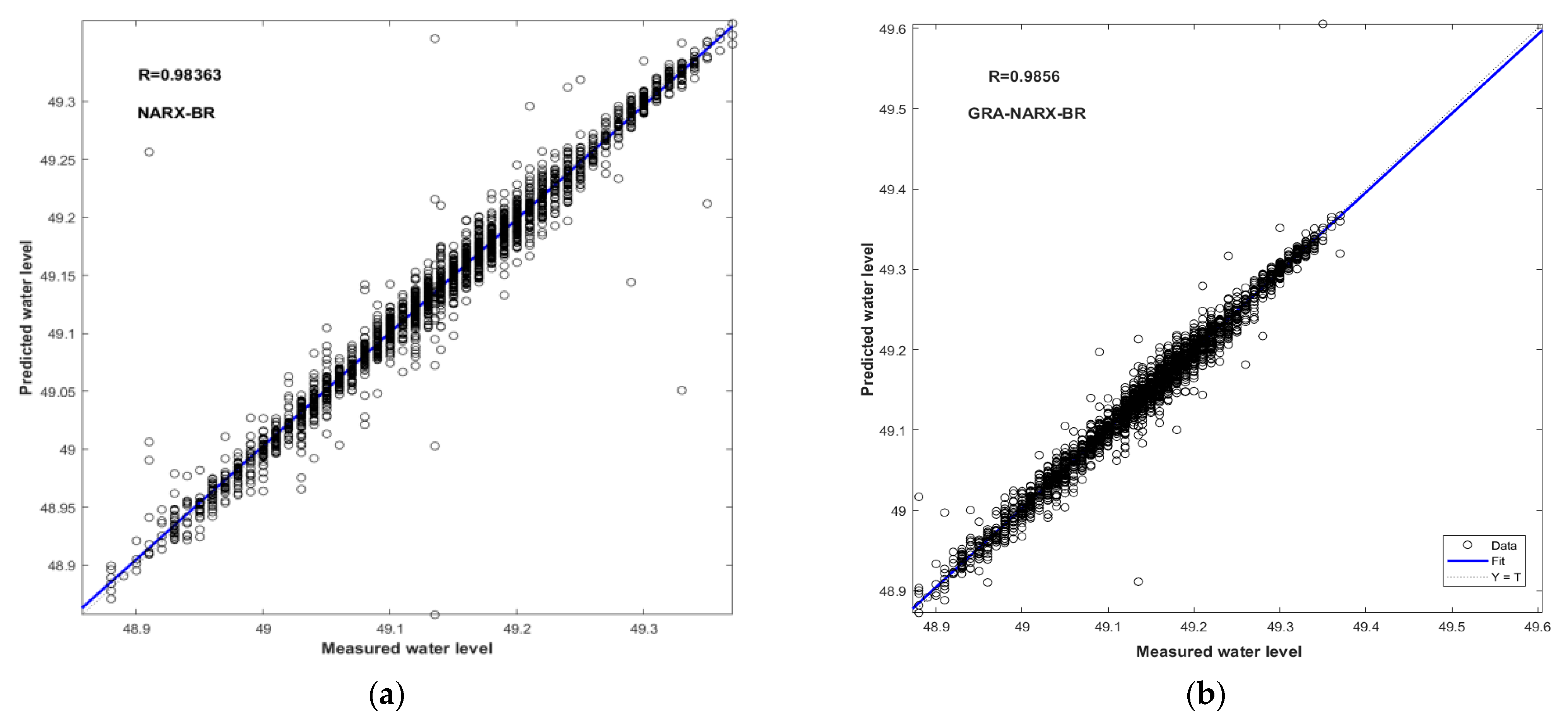
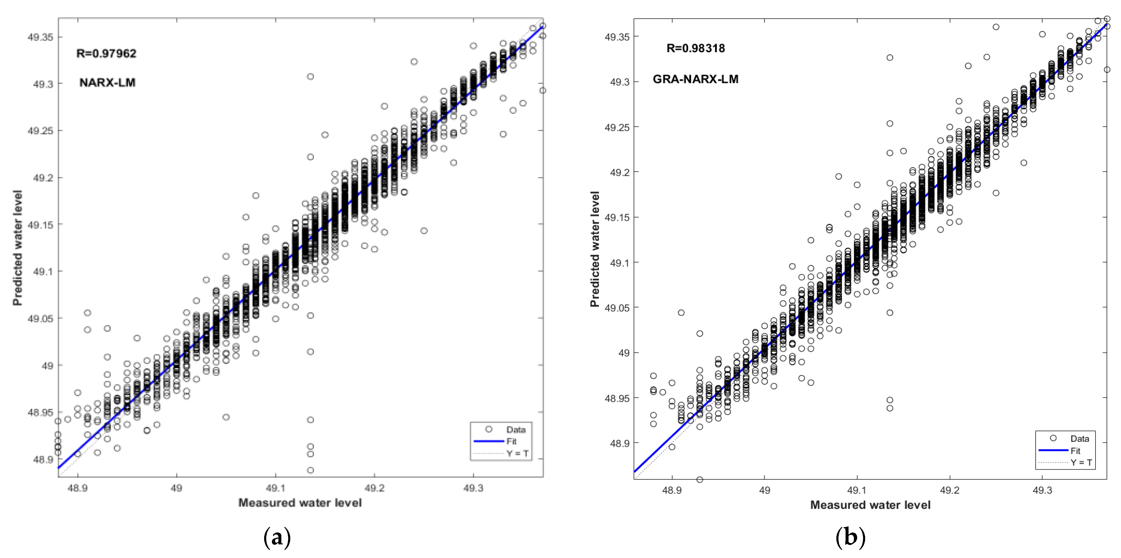
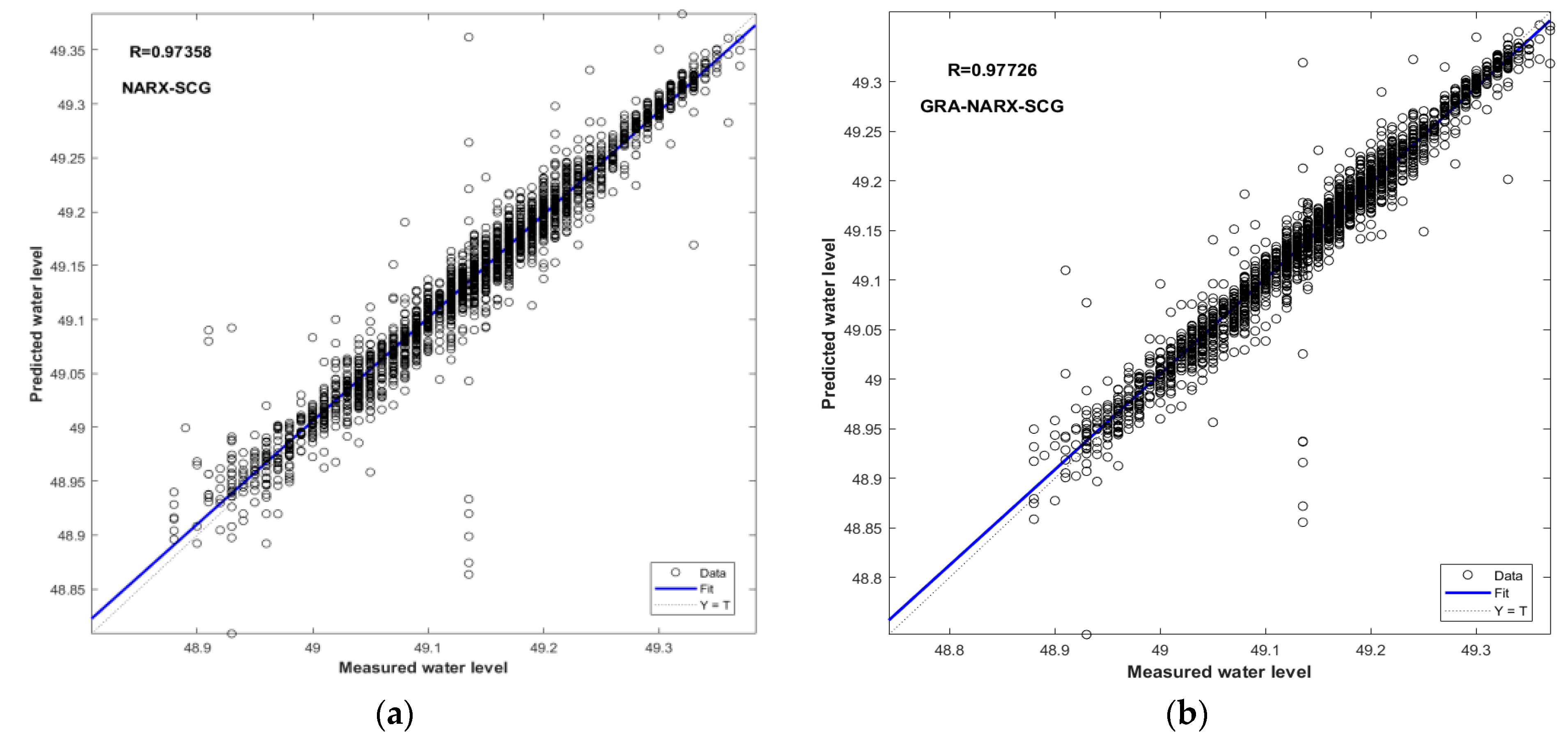
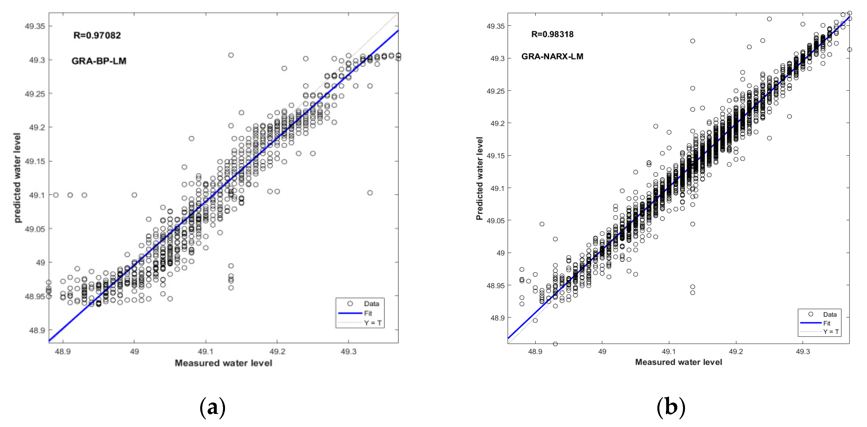
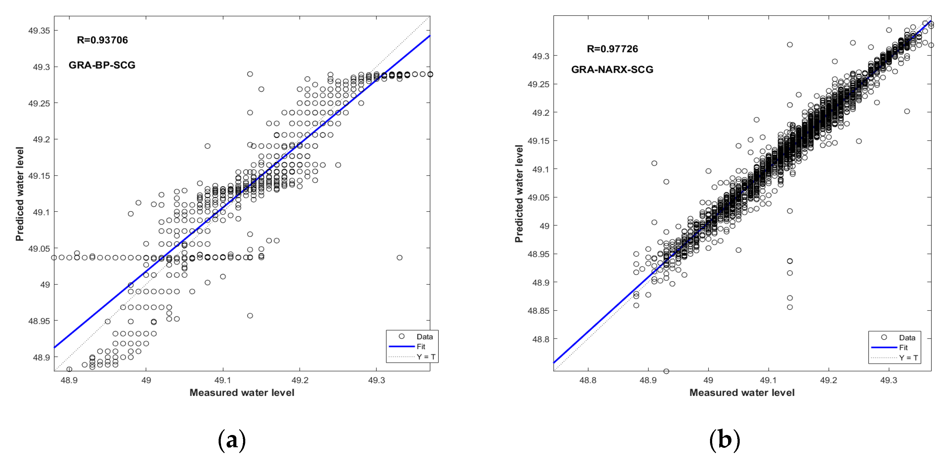
As seen in Figure 6, Figure 7 and Figure 8, the index R serves as a summary and evaluation of the NARX and GRA–NARX models’ performances. In comparison to the NARX model, it is discovered that the GRA-NARX model is more reliable irrespective of the training algorithm used. Under the optimal combination of the time delay and the hidden neurons number, the R values are 0.9856 and 0.98363 for the GRA-NARX and NARX models using BR as the training algorithm, 0.98318 and 0.97962 for that using LM as the training algorithm, and 0.97726 and 0.97358 for that using SCG as the training algorithm, respectively.

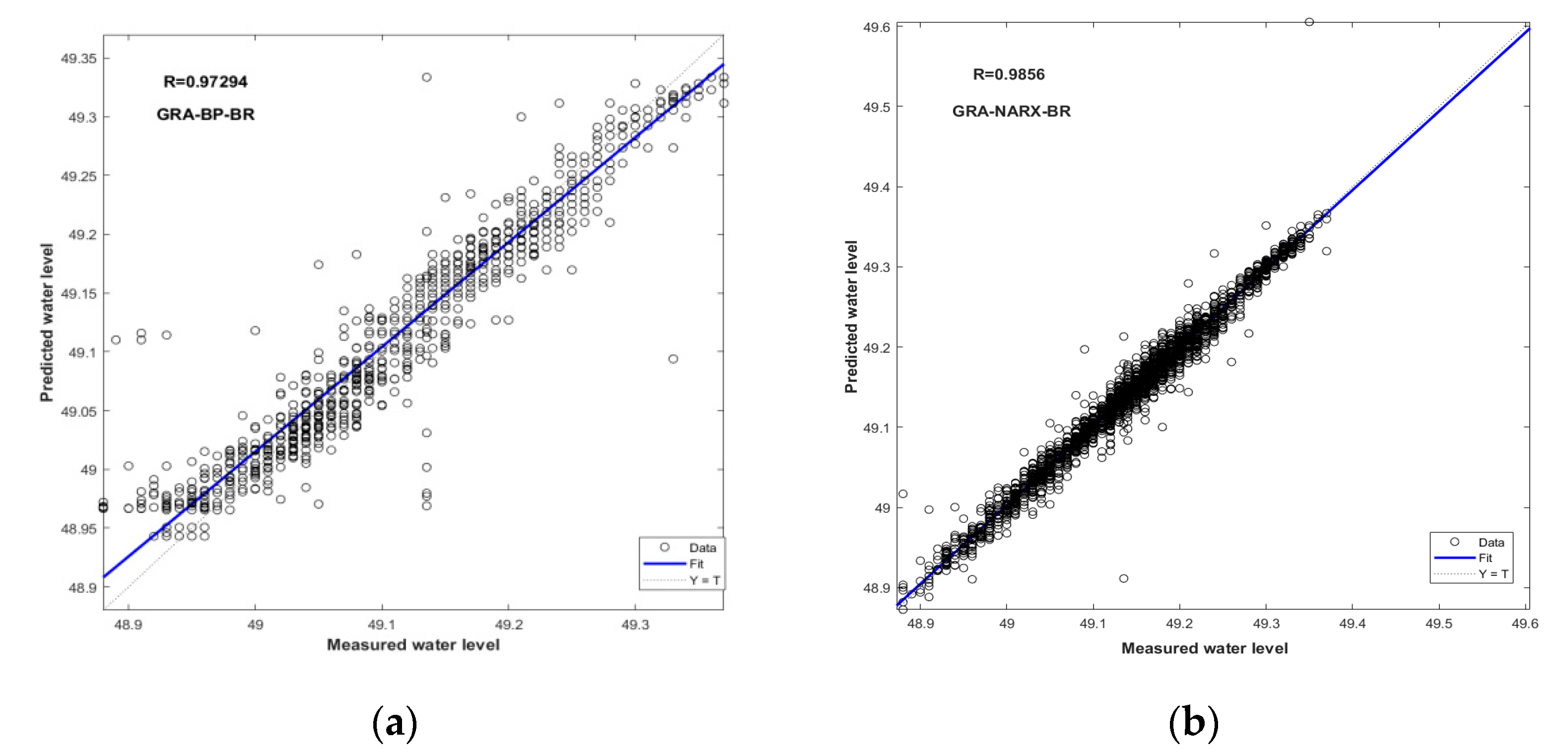
The comparison of the performance between the GRA-BP and GRA-NARX models using BR, LM, and SCG as the training algorithms is illustrated in Figure 9, Figure 10 and Figure 11, respectively. Again, the GRA-NARX model is more accurate than the GRA-BP model irrespective of the training algorithm used. Under the optimal combination of the time delay and the hidden neurons number, the R values are 0.9856 and 0.97294 for the GRA-NARX and GRA-BP models using BR as the training algorithm, 0.98318 and 0.97082 for that using LM as the training algorithm, and 0.97726 and 0.93706 for that using SCG as the training algorithm, respectively.

Table 4. The MSE and MAE values for the three models with different training algorithms.

Training Algorithm	GRA-NARX		GRA-BP		NARX
	MSE	MAE	MSE	MAE	MSE	MAE
BR LM SCG	2.3104 × 10−4 2.9929 × 10−4 4.7089 × 10−4	0.00984 0.01216 0.01288	5.7121 × 10−4 7.1824 × 10−4 9.8596 × 10−4	0.01754 0.02080 0.02559	2.3716 × 10−4 4.5796 × 10−4 4.7961 × 10−4	0.01042 0.01289 0.01324

shows the MSE and MAE values for the GRA-NARX, GRA-BP, and NARX models with different training algorithms under the optimal combination of the time delay and the hidden neurons number. When BR is used as the training algorithm, the MSE is 2.3104 × 10⁻⁴, 5.7121 × 10⁻⁴, and 2.3716 × 10⁻⁴ with MAE of 0.00984, 0.01754, and 0.01042 for the GRA-NARX, GRA-BP, and NARX models, respectively; when LM is used as the training algorithm, the MSE is 2.9929 × 10⁻⁴, 7.1824 × 10⁻⁴, and4.5796 × 10⁻⁴ with MAE of 0.01216, 0.02080, and 0.01289 for the GRA-NARX, GRA-BP and NARX models, respectively; and when SCG is used as the training algorithm, the MSE is 4.7089 × 10⁻⁴, 9.8596 × 10⁻⁴, and 4.7961 × 10⁻⁴ with MAE of 0.01288, 0.02559, and 0.01324 for the GRA-NARX, GRA-BP, and NARX models, respectively.

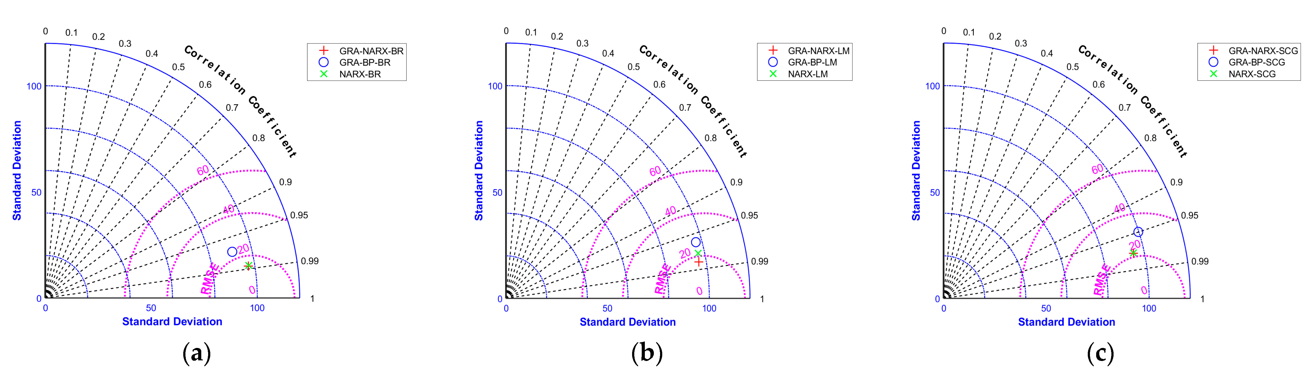
In addition, Taylor diagrams [39] are used to assess the three models’ performances (Figure 12). Figure 12 exhibits the higher performance of the GRA-NARX model, with both the lowest RMSE value and the best correlation coefficient. The GRA-NARX-BR model can be regarded as the best model for the water-level prediction of a pumping station forebay.

The performances of the three models with different training algorithms are further compared by means of MSE and MAE in the training, validation, and test periods (

Table 5. The MSE and MAE values for the three models with different training algorithms in the training, validation, and test periods.

Samples	Training Algorithm	GRA-NARX		GRA-BP		NARX
		MSE	MAE	MSE	MAE	MSE	MAE
Training	BR LM SCG	1.5449 × 10−4 1.9321 × 10−4 2.6244 × 10−4	0.0092 0.0096 0.0110	3.2041 × 10−4 5.1076 × 10−4 5.4289 × 10−4	0.0135 0.0216 0.0186	1.6129 × 10−4 2.4649 × 10−4 2.9929 × 10−4	0.0096 0.0107 0.0115
Validation	BR LM SCG	1.4884 × 10−4 1.7689 × 10−4 2.2500 × 10−4	0.0094 0.0093 0.0113	4.7961 × 10−4 8.2369 × 10−4 8.5884 × 10−4	0.0193 0.0227 0.0232	1.801 × 10−4 2.4964 × 10−4 4.621 × 10−4	0.0091 0.0107 0.0123
Test	BR LM SCG	4.2436 × 10−4 9.0000 × 10−4 1.6892 × 10−3	0.0111 0.0167 0.0250	1.6241 × 10−3 1.4516 × 10−3 3.2149 × 10−3	0.0259 0.0267 0.0413	7.3441 × 10−4 4.7961 × 10−3 1.5445 × 10−3	0.0121 0.0233 0.0250

). Under the optimal combination of the time delay and the hidden neurons number, we can see from Table 5 that the GRA-NARX model is more accurate than other models. For instance, it can be demonstrated that over the training period the GRA-NARX-BR model has the smallest MSE (1.5449 × 10⁻⁴) and MAE (0.0092). The results from the GRA-BP-BR model are, respectively, an MSE of 3.2041 × 10⁻⁴ and an MAE of 0.0135, and from the NARX-BR model, an MSE of 1.6129 × 10⁻⁴ and an MAE of 0.0096.

4. Discussion

The results demonstrate that the novel GRA-NARX model is effective for predicting the water levels in front of the Tundian pumping station.

Figure 6, Figure 7, Figure 8, Figure 9, Figure 10 and Figure 11 depict that the correlation of the GRA-NARX model is further improved. From the MSE and MAE values for the three models (Table 4), we find that GRA-NARX model has the smallest MSE and MAE values. Bedsides, the more comparable representation of the model performance is shown by the Taylor diagram (Figure 12). The GRA-NARX model is closest to the observed site, whereas the GRA-BP model was situated the farthest away. At the same time, we give the estimation results of the three models in the training, validation, and test periods (Table 5). The GRA-NARX model has smaller MSE and MAE values than the GRA-BP model and the NARX model, which reveals that the GRA-NARX model has a good generalization ability. The novel GRA-NARX model can also be utilized to solve other prediction problems because of its distinctive structural features and the improved algorithm of the NARX neural network. It will perform better than many other models.

In comparison to earlier studies, our results are favorable. A classification—nonlinear auto-regressive exogenous (C-NARX) model based on runoff classification and NARX was used to predict the Linyi watershed’s runoff in the Huaihe River’s northeastern section. With two input variables, one hidden layer, ten hidden neurons, and five-time delay based on experience, the NARX model’s ideal architecture was established. The minimum of MSE was 4.12 × 10⁻² [36]. In our study, the optimal combination of the time delay and the hidden neurons number was obtained by the improved algorithm and the minimum of MSE was 1.975 × 10⁻⁴. The results are satisfactory, and the proposed model is interpretable.

Although good results are obtained for water level prediction using the GRA-NARX model in the study area, there are still some limitations. For example, Chen et al. [40,41] evaluated the performance of the ANN approach with hydrodynamic models, they got some promising results. While in our investigation, the GRA-NARX model was only compared with ANN models.

5. Conclusions

The GRA-NARX model is proposed in this study based on GRA and the NARX neural network for a 2 h ahead prediction of water levels in front of pumping stations, and an improved algorithm is used to obtain the optimal combination of the time delay and the hidden neurons number. The sensitivity to changes of the training algorithm is analyzed, and the prediction performance is compared with that of the NARX and GRA-BP models. A case study is performed in the Tundian pumping station of the Miyun Reservoir project to demonstrate the reliability and accuracy of the proposed model. The main conclusions are as follows:

(1)

The optimal combination of the time delay and the hidden neurons number is obtained by the GRA-NARX model with different training algorithms to minimize the MSE.

(2)

The novel GRA-NARX neural network can reduce the prediction complexity and improve the prediction accuracy. The model is applicable to the water-level prediction of the water transfer project with the correlation coefficient of up to 0.98662 and the minimum MAE of 0.00984 m.

(3)

The GRA-NARX neural network using BR as the training algorithm (the GRA-NARX-BR model) shows the highest R and the smallest MSE in the prediction of the water level in front of the Tundian pumping station. It is more accurate than the NARX and GRA-BP models and has less run time than the NARX model.

There are still some issues that warrant future research: (1) the novel GRA-NARX model will be compared with a numerical model; (2) since there are numerous variables influencing the water levels in front of a pumping station, it is important to further evaluate the complexity and variety of the model; and (3) it is possible to create additional possibilities by using a wider range of the time delay and the number of hidden neurons.

References

- Wei, X.; Chen, C. Optimization of operation strategies for an inter basin water diversion system using an aggregation model and improved NSGA-II algorithm. J. Irrig. Drain. Eng. 2020, 146, 04020006. [Google Scholar] [CrossRef]
- Munar, A.M.; Cavalcanti, J.R.; Bravo, J.M.; Fan, F.M.; Motta-Marques, D.D.; Fragoso, C.R. Coupling large-scale hydrological and hydrodynamic modeling: Toward a better comprehension of watershed-shallow lake processes. J. Hydrol. 2018, 564, 424–441. [Google Scholar] [CrossRef]
- Lei, X.; Tian, Y.; Zhang, Z.; Wang, L.; Xiang, X.; Wang, H. Correction of pumping station parameters in a one-dimensional hydrodynamic model using the Ensemble Kalman filter. J. Hydrol. 2019, 568, 108–118. [Google Scholar] [CrossRef]
- Tao, H.; Al-Bedyry, N.K.; Khedher, K.M.; Shahid, S. River water level prediction in coastal catchment using hybridized relevance vector machine model with improved grasshopper optimization. J. Hydrol. 2021, 598, 126477. [Google Scholar] [CrossRef]
- Lin, Y.H.; Chiu, C.C.; Lin, Y.J.; Lee, P.C. Rainfall prediction using innovative grey model with the dynamic index. J. Mar. Sci. Tech. 2013, 21, 9. [Google Scholar] [CrossRef]
- Sahoo, S.; Jha, M.K. Groundwater-level prediction using multiple linear regression and artificial neural network techniques: A comparative assessment. Hydrogeol. J. 2013, 21, 1865–1881. [Google Scholar] [CrossRef]
- Liu, Y.; Wang, H.; Feng, W.; Huang, H. Short term real-time rolling forecast of urban river water levels based on lSTM: A case study in fuzhou city, China. Int. J. Environ. Res. Public Health 2021, 18, 9287. [Google Scholar] [CrossRef]
- Tang, M.; Lei, X.H.; Long, Y. Water level forecasting in middle route of the south-to-north water diversion project Based on Long Short-term Memory. China Rur. Wat. Hydrop. 2020, 10, 189–193. [Google Scholar]
- Páliz Larrea, P.; Zapata-Ríos, X.; Campozano Parra, L. Application of neural network models and ANFIS for water level forecasting of the Salve Faccha Dam in the Andean Zone in Northern Ecuador. Water 2021, 13, 2011. [Google Scholar] [CrossRef]
- Alsumaiei, A.A. A nonlinear autoregressive modeling approach for forecasting groundwater level fluctuation in urban aquifers. Water 2020, 12, 820. [Google Scholar] [CrossRef]
- Reitz, M.; Sanford, W.E. Estimating quick-flow runoff at the monthly timescale for the conterminous United States. J. Hydrol. 2019, 573, 841–854. [Google Scholar] [CrossRef]
- Tu, Z.J.; Gao, X.G.; Xu, J.; Sun, W.; Sun, Y.; Su, D. A novel method for regional short-term forecasting of water level. Water 2021, 13, 820. [Google Scholar] [CrossRef]
- Barzegar, R.; Aalami, M.T.; Adamowski, J. Coupling a hybrid CNN-LSTM deep learning model with a Boundary Corrected Maximal Overlap Discrete Wavelet Transform for multiscale Lake water level forecasting. J. Hydrol. 2021, 598, 126196. [Google Scholar] [CrossRef]
- Ren, T.; Liu, X.F.; Niu, J.W.; Lei, X.H.; Zhangm, Z. Real-time water level prediction of cascaded channels based on multilayer perception and recurrent neural network. J. Hydrol. 2020, 585, 124783. [Google Scholar] [CrossRef]
- Pandey, K.; Kumar, S.; Malik, A.; Kuriqi, A. Artificial neural network optimized with a genetic algorithm for seasonal groundwater table depth prediction in Uttar Pradesh, India. Sustainability 2020, 12, 8932. [Google Scholar] [CrossRef]
- Xiong, B.; Li, R.P.; Ren, D.; Liu, H.; Xu, T.; Huang, Y. Prediction of flooding in the downstream of the Three Gorges Reservoir based on a back propagation neural network optimized using the AdaBoost algorithm. Nat. Hazards 2021, 107, 1559–1575. [Google Scholar] [CrossRef]
- Tian, Y.; Xu, Y.P.; Yang, Z.; Wang, G.; Zhu, Q. Integration of a parsimonious hydrological model with recurrent neural networks for improved stream flow forecasting. Water 2018, 10, 1655. [Google Scholar] [CrossRef]
- Zhang, J.F.; Zhu, Y.; Zhang, X.P.; Ye, M.; Yang, J. Developing a Long Short-Term Memory(LSTM) based model for predicting water table depth in agricultural areas. J. Hydrol. 2018, 561, 918–929. [Google Scholar] [CrossRef]
- Baek, S.S.; Pyo, J.C.; Chun, J.A. Prediction of water level and water quality using a CNN-LSTM combined deep learning approach. Water 2020, 12, 3399. [Google Scholar] [CrossRef]
- Wu, M.L.; Yang, K.; Zhang, C.C. Application of KG-BP neural network in flood forecasting of Qinhuai River. Water Resour. Powerpoint 2019, 37, 74–77. [Google Scholar]
- Li, P.; Zhang, J.; Krebs, P. Prediction of Flow Based on a CNN-LSTM Combined Deep Learning Approach. Water 2022, 14, 993. [Google Scholar] [CrossRef]
- Li, C.; Zhu, L.; He, Z.; Gao, H.; Yang, Y.; Yao, D.; Qu, X. Runoff prediction method based on adaptive Elman neural network. Water 2019, 11, 1113. [Google Scholar] [CrossRef] [Green Version]
- Chen, S.; BilliIngs, S.A. Non-linear system identification using neural networks. Int. J. Control 1990, 51, 1191–1214. [Google Scholar] [CrossRef]
- Desouky, M.A.; Abdelkhalik, O. Wave prediction using wave rider position measurements and NARX network in wave energy conversion. Appl. Ocean Res. 2019, 82, 10–21. [Google Scholar] [CrossRef]
- Guzman, S.M.; Paz, J.O.; Tagert, M.L.M. The use of NARX neural networks to forecast daily groundwater levels. Water Resour. Manag. 2017, 31, 1591–1603. [Google Scholar] [CrossRef]
- Di Nunno, F.; Granata, F.; Gargano, R. Forecasting of Extreme Storm Tide Events Using NARX Neural Network-Based Models. Atmosphere 2021, 12, 512. [Google Scholar] [CrossRef]
- Di Nunno, F.; Granata, F. Groundwater level prediction in Apulia region (Southern Italy) using NARX neural network. Environ. Res. 2020, 190, 110062. [Google Scholar] [CrossRef]
- Wunsch, A.; Liesch, T.; Broda, S. Forecasting groundwater levels using nonlinear autoregressive networks with exogenous input (NARX). J. Hydrol. 2018, 567, 743–758. [Google Scholar] [CrossRef]
- Ezzeldin, R.; Hatata, L. Application of NARX neural network model for discharge prediction through lateral orifices. Alex. Eng. J. 2018, 57, 2991–2998. [Google Scholar] [CrossRef]
- Wang, J.L.; Chen, Y. Using NARX neural network to forecast droughts and floods over Yangtze River Basin. Nat. Hazards 2022, 110, 225–246. [Google Scholar] [CrossRef]
- Fan, Z.N.; Liu, X.S. Application of NARX neural network in dam deformation prediction. J. Yellow River 2022, 44, 125–128. [Google Scholar] [CrossRef]
- Chen, Z.X.; Wang, D. A prediction model of forest preliminary precision fertilization based on improved GRA-PSO-BP neural network. Math. Probl. Eng. 2020, 2020, 1356096. [Google Scholar] [CrossRef]
- Chen, B.; Lin, P.; Lin, Y.; Lai, Y.; Cheng, S.; Chen, Z.; Wu, L. Hour-ahead photovoltaic power forecast using a hybrid GRA-LSTM model based on multivariate meteorological factors and historical power datasets. Conf. Ser. Earth Environ. Sci. 2020, 431, 012059. [Google Scholar] [CrossRef]
- Zhou, T.Y.; Xu, Q.; Liu, Z.Z. Time-series dissolved oxygen prediction based on optimized NARX neural network. J. Donghua Univ. 2021, 48, 16710444. [Google Scholar]
- Di Nunno, F.; De Marinis, G.; Gargano, R.; Granata, F. Tide prediction in the Venice Lagoon using nonlinear autoregressive exogenous (NARX) neural network. Water 2021, 13, 1173. [Google Scholar] [CrossRef]
- Shao, Y.; Zhao, J.; Xu, J.; Fu, A.; Li, M. Application of rainfall-runoff simulation based on the NARX dynamic neural network model. Water 2022, 14, 2082. [Google Scholar] [CrossRef]
- Smiti, A. A critical overview of outlier detection methods. Comput Sci. Rev. 2020, 38, 100306. [Google Scholar] [CrossRef]
- Di Nunno, F.; Granata, F.; Gargano, R.; de Marinis, G. Prediction of spring flows using nonlinear autoregressive exogenous (NARX) neural network models. Environ. Monit. Assess. 2021, 193, 350. [Google Scholar] [CrossRef]
- Elbeltagi, A.; Di Nunno, F.; Kushwaha, N.L.; De Marinis, G. River flow rate prediction in the Des Moines watershed (Iowa, USA): A machine learning approach. Stoch. Env. Res. Risk A. 2022, 1–21. [Google Scholar] [CrossRef]
- Liu, W.C.; Chen, W.B. Prediction of water temperature in a subtropical subalpine lake using an artificial neural network and three-dimensional circulation models. Comput. Geosci. 2012, 45, 13–25. [Google Scholar] [CrossRef]
- Chen, W.B.; Liu, W.C.; Hsu, M.H. Comparison of ANN approach with 2D and 3D hydrodynamic models for simulating estuary water stage. Adv. Eng. Softw. 2012, 45, 69–79. [Google Scholar] [CrossRef]
Figure 1.
A schematic diagram of the Miyun Reservoir project.
Figure 2.
A schematic diagram of the box plot.
Figure 3.
The structure of the NARX neural network.
Figure 4.
The flowchart of the GRA-NARX model.
Figure 5.
Thermal diagram of the mean square errors obtained by different training algorithms under different combinations of the time delay and the hidden neurons number: (a) use of BR as the training algorithm, (b) use of LM as the training algorithm, and (c) use of SCG as the training algorithm.
Figure 6.
Scatter plots of measured and predicted water levels for the GRA-NARX and NARX models using BR as the training algorithm: (a) NARX-BR, (b) GRA-NARX-BR.
Figure 7.
Scatter plots of measured and predicted water levels for the GRA-NARX and NARX models using LM as the training algorithm: (a) NARX-LM, (b) GRA-NARX-LM.
Figure 8.
Scatter plots of measured and predicted water levels for the GRA-NARX and NARX models using SCG as the training algorithm: (a) NARX-SCG, (b) GRA-NARX-SCG.
Figure 9.
Scatter plots of measured and predicted water levels for the GRA-NARX and GRA-BP models using BR as the training algorithm: (a) GRA-BP-BR, (b) GRA-NARX-BR.
Figure 10.
Scatter plots of measured and predicted water levels for the GRA-NARX and GRA-BP models using LM as the training algorithm: (a) GRA-BP-LM, (b) GRA-NARX-LM.
Figure 11.
Scatter plots of measured and predicted water levels for the GRA-NARX and GRA-BP models using SCG as the training algorithm: (a) GRA-BP-SCG, (b) GRA-NARX-SCG.
Figure 12.
Taylor plots of measured and predicted water levels: (a) use of BR as the training algorithm, (b) use of BR as the training algorithm, and (c) use of BR as the training algorithm.