1. Introduction
Resources must be used in such a way that the balance between their use and sustainability is maintained. As water is a necessary component for the continuation of all forms of life on Earth, any effort to achieve this balance is important. In the management of reservoirs, this means increasing the benefits for the population, such as access to services of drinking water, electricity and the development of economic and recreational activities. Nonetheless, external factors such as climatic change increase the occurrence of hurricanes and tropical storms, bringing unusual rainfall or lengthy droughts that affect the functioning of reservoirs, leading to spills and deficiency situations, flooding downstream, damage to reservoir systems, loss of human and animal life, crop damage, disease, water pollution and scarcity of water.
In general, optimizing techniques and quicker computing equipment have been beneficial in reservoir management. The combination of both tools helps in integrating the physical constraints of the system, penalizations for spillage and water scarcity, resource maximization, more accurate models and forecasting and obtaining solutions quickly.
One such technique is dynamic programming (DP), developed by [
1] and applied in a variety of fields, including the optimization of single and multi-reservoir systems. Examples of studies on this subject in other parts of the world include: [
2] (China); [
3] (Iran); [
4] (Taiwan); [
5], (India); [
6] (Sri Lanka); [
7] (Australia); [
8] (USA); [
9] (Germany); [
10] (Korea); [
11] (Spain); [
12] (Africa: Zambezi river basin); [
13] (Iraq); [
14] (Norway).
However, since DP is an iterative method, there is a risk of not finding unique solutions and thus becoming trapped in eternal cycles that only find solutions when the number of iterations is reached and, because it is also an algorithm that requires great computational resources, it is critical to properly establish the stopping mechanism. With this in mind, the present study examines two stopping trials in optimizing operational rules, in a reservoir cascade system, using the DP algorithm in its stochastic variation (SDP).
We identified studies on in a literature review, including [
2,
15,
16,
17,
18,
19,
20,
21,
22,
23]. These works helped us to establish the two trials described in this study. The literature review and several recent works carried out at the UNAM Engineering Institute revealed the importance of the convergence criterion used when seeking optimum solutions for multi-reservoir systems with a large storage capacity. In this study, two trials are analysed in order to achieve convergence that guarantees stability of the solution and to reduce computational time.
The study is divided thus:
Section 2 presents the general features of DP and the two stopping strategies defined to obtain the operation rule.
Section 3 describes the study site and explains the process conditions to optimize and simulate the reservoir system. In
Section 4 the results obtained are presented, then in
Section 5 conclusions are given.
2. Methodology
2.1. Background and Theoretical Framework
The works of [
24,
25], which have studied a multi-reservoir system by determining optimal policies, using as a convergence criterion that the absolute value of the differences between two consecutive iterations is less than a given tolerance value, will be taken as a starting point. Both studies use the dynamic programming methodology, a technique developed by [
26] that can be used if and only if the solutions of the problem to be solved constitute a series of decisions. The calculations are carried out in a recursive manner [
27,
28]. The details of the theory for both the deterministic and stochastic cases are widely discussed in the literature [
26,
29,
30,
31,
32].
To obtain the operation policies the following considerations were taken:
The goal was to maximize the expected annual energy generation from the system and avoid spills and events where the demands are not met (called deficit events)
where
E denotes expectation,
T number of periods within the annual cycle (stages),
EG energy generation (GWh),
C penalization coefficient,
OE occurred event (spill or deficit), and
nr number of reservoirs.
- (b)
Constraints.
- b.1
Storage
where
Smin minimum storage of reservoir,
Smax maximum storage of reservoir, and S reservoir storage.
- b.2
Release
where
Rmin = minimum release from the reservoir,
Rmax maximum release from the reservoir,
R release from the reservoir
- (c)
State transformation equations.
The equations are obtained according to the principle of continuity [
32]
where
Se is storage at the end of the stage,
Sb storage at the beginning of the stage,
I inflow to reservoir
i,
r release from reservoir
i, and
O losses (principally evaporation). It should be taken into account that, when the system operates in cascade, the downstream reservoir will have as additional income the volumes spilled by that which precedes it.
- (d)
Recursive equations for a multi-reservoir system [
25,
32]
where
k is the storage state space;
l decision space; p inflow state space during period
j;
q inflow state space during period
j + 1;
accumulated expected energy generation by optimal operation of the system over the last n stages; B benefit for energy generation when system changes from state
ki to state
li when inflow class is
pi in period
j;
JP joint transition probabilities of inflows.
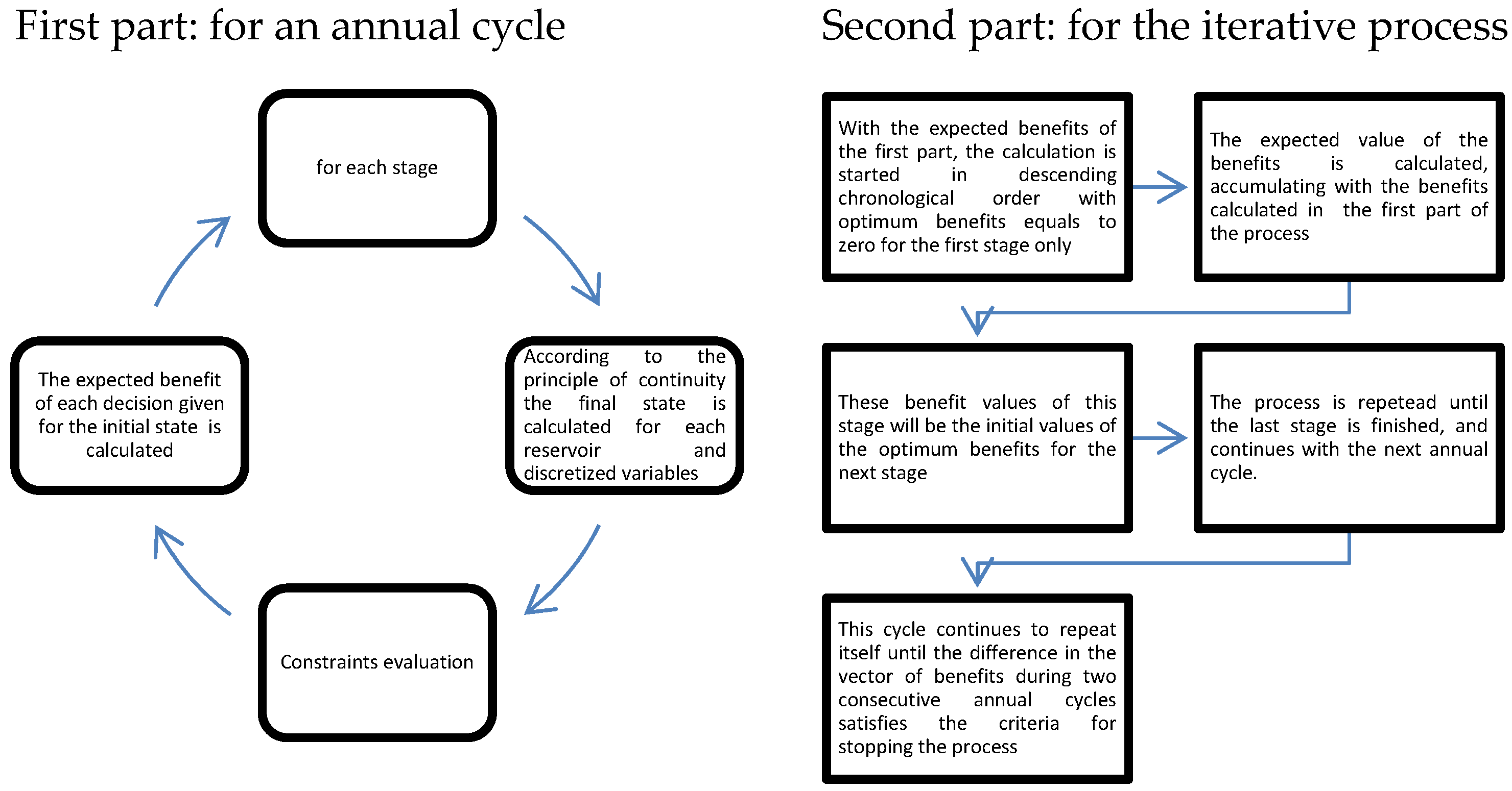
The disadvantage of DP is the high cost of computational resources it demands; to avoid this, the technique used in II UNAM splits the solution procedure into two parts: only the expected benefit is calculated for each stage (first term of Equation (5)), which is repeated from one year to another, in the first part; the accumulated benefit up to the considered stage and its optimum value are determined, for which a very large number of years is proposed (which may correspond to the normal life of the system), in the second part (second term of Equation (5)). In the initial stage, values of zero are assigned to the optimum benefits, the stages are started in the opposite direction to time and the equations are solved by iterating until the differences between two consecutive years meet an established tolerance that guarantees convergence and stability for the solution. Once this is achieved, the optimal release policy for each dam is stored, along with its respective benefit [
24].This process is illustrated in
Figure 1:
2.2. Convergence Criterion
According to the literature, an incremental solution strategy based on an iterative method will be effective if, and only if, the selection of the convergence criterion is adequate for the completion of the iteration process. It is recommended to keep in mind that not complying with the convergence criterion may lead to not quite accurate results, a very strict tolerance criterion will have an increased computation time and the solution may not need such thoroughness.
In this study, two convergence criteria were formulated to identify the optimal operation policies for a multi-reservoir system, which consists of four reservoirs. The recursion equations of the stochastic dynamic programming method are applied until the criterion is met or the number of iterations corresponding to the normal life of the system is reached.
From [
24,
25,
28] the convergence criterion used was
where
t is time (one full year, in this case);
V(
Xt) denotes value function and µ is tolerance.
The value of μ chosen was fixed at 10
−3. However, according to the literature, adding a discount factor that is a real number between 0 and 1 is recommended. Then, a typical convergence criterion is [
18,
33]
where
β is a discount factor.
Using Equation (7) we define two trials to analyse how different are the optimized values for the policy, the spent time and the behaviour of the chosen system during the simulation using the historic record of inflows. The trials are defined as follows:
Trial 1: The first stopping strategy involves adding the absolute value of the differences between two subsequent values, for all possible states, then taking the average and comparing it to the convergence criterion at the end of two cycles
where
D is a vector in which the differences of two consecutive cycles are accumulated,
T is the total number of groups of months in which the year was divided, and
tns is the total number of states, considering the two reservoirs.
- 2
Trial 2: Instead of taking the absolute value, the second strategy was to square the differences
The iterative process is carried out until one of the defined conditions is met: by reaching the maximum number of iterations, or by meeting the convergence criterion. The results of the two trials are shown in
Section 4.
3. Case Study
3.1. Multi-Reservoir System
The reservoir system examined is on the Grijalva River in southeast Mexico (
Figure 2). The river begins in Guatemala and flows through the state of Chiapas in Mexico, then a for a further 480 km to its mouth in the Gulf of Mexico [
34]. The administrative bounds of the basin include the states of Tabasco, Chiapas and small portions of Campeche, covering a total area of 52,348 km
2, part of the “Grijalva-Usumacinta” hydrological region 30.
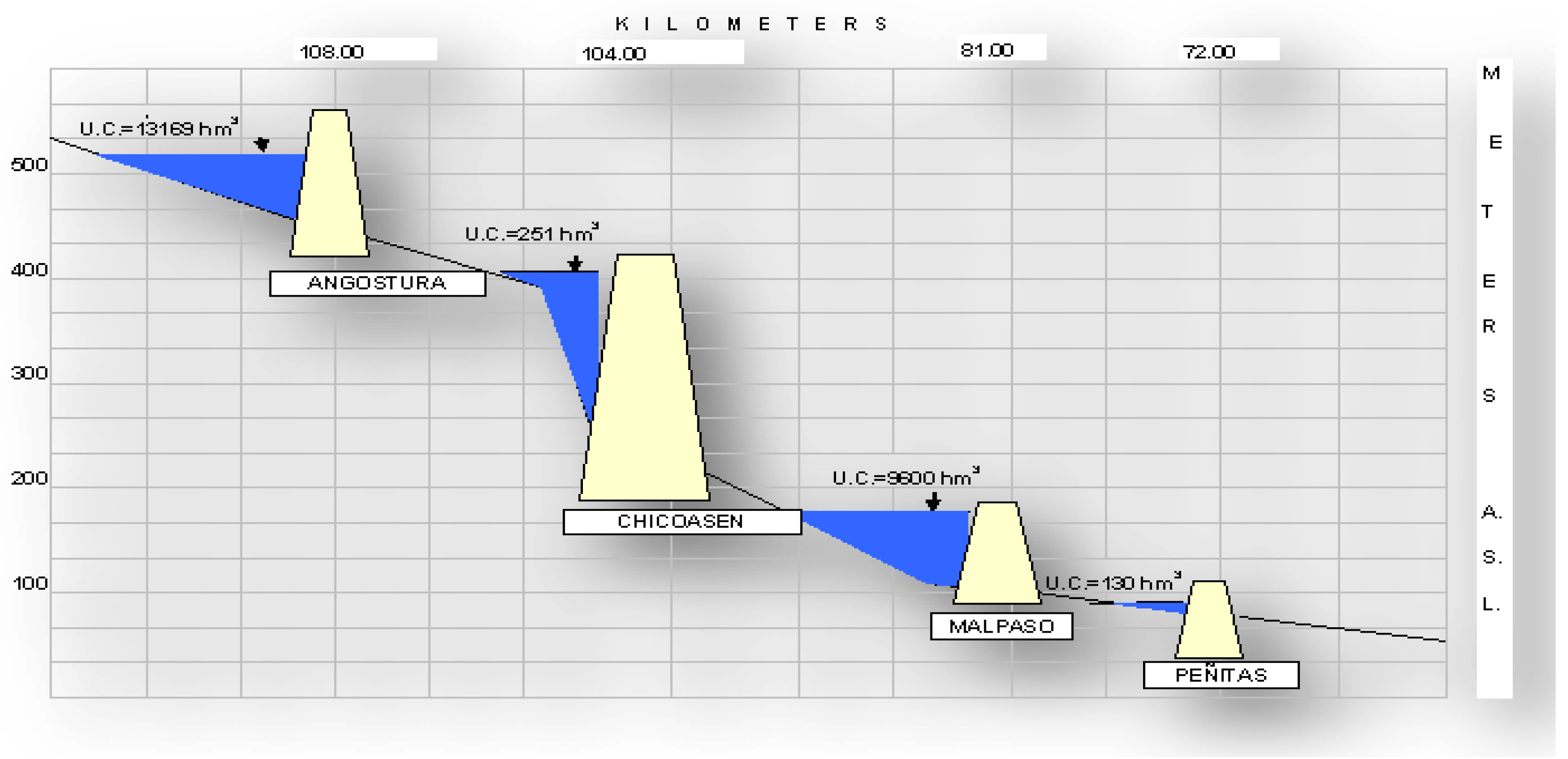
Between 1959 and 1987, four dams were built on the river Grijalva.
Figure 3 shows the layout of the dams that make up the system and their storage capacities.
- (a)
La Angostura was built between 1969 and 1975. Its main uses are flood control, hydroelectric power generation, agricultural irrigation and domestic water supply, fishing and tourism.
- (b)
Chicoasén was built between 1977 and 1983. Its main uses are hydroelectric power generation, agricultural irrigation and domestic water supply, fishing, national and international tourism and water sports.
- (c)
Malpaso was built between 1959 and 1964. Its main uses are electricity generation and flood control.
- (d)
Peñitas is located in the municipality of Ostuacán, Chiapas. It was completed in 1987. The production of electricity is its primary function.
With normal storage capacities of 13,169 and 9600 hm
3, respectively, La Angostura and Malpaso dams are the largest of the complex [
25]. In terms of electricity generation, the installed capacity of the system (3907 MW) represents 40.3% of the national hydroelectric capacity and 52% of the energy generated by Mexican hydroelectric plants [
36].
3.2. Optimization and Simulation Processes
The optimization process uses a series of assumptions in order to obtain the operation policies of the dams. It is important to simplify the management of the four-dam system of the Grijalva River, to optimize the two main dams. There is a great difference in the storage capacities of La Angostura and Malpaso and of Chicoasén and Peñitas; if we take this into account, then the smaller dams should be considered as diversion dams only, and their operation policy will consist of releasing the volumes that pass through them, taking into account physical restrictions. The volumes of water entering Chicoasén are added to those of Malpaso (which is downstream) and the energy generated by Chicoasén and Peñitas is considered by adding their hydraulic heads to La Angostura and Malpaso, respectively. This simplification significantly reduces the complexity of the system but maintains the actual operating conditions of the four reservoirs.
Once the policies are obtained, the operation of the multi-reservoir system is simulated using them, the physical characteristics of the system and the record of historic inflows.
The conditions for the optimization and simulation processes are described in [
24,
25,
28], and the most important are listed in summaries 2 and 3.
Summary 2. Optimization process
Six stages were defined to group the 12 months of the year (
Table 1)
A value of 600 hm3 (ΔV) was selected to discretize the state variables, thus, the number of states in which the normal storage capacity of La Angostura was discretized was 22, with 16 for Malpaso.
The months of each stage and the maximum and minimum releases are shown in
Table 1. These last values were determined as follows: the drinking water supply is a minimum release of 200 m
3/s for La Angostura, and 300 m
3/s for Malpaso. The maximum is determined by taking the maximum monthly turbine discharge, in this case, 2825 hm
3 for La Angostura and 3732 hm
3 for Malpaso. As example for stage 1 and La Angostura dam, the minimum and maximum releases are as follows: 200 m
3/s must be expressed in hm
3/month and then in volume discretization units to obtain the minimum release per month, i.e.,
Stage 1 has 2 months: Nov and Dec, therefore the minimum release will be
The same procedure is applied to obtain the maximum release, but taking the maximum monthly turbine discharge now, i.e.,
Then for 2 months, the maximum release will be
In the case of Malpaso, to obtain the minimum and maximum releases for a stage that has, for example, a single month
Following this process, the values shown in
Table 1 are obtained.
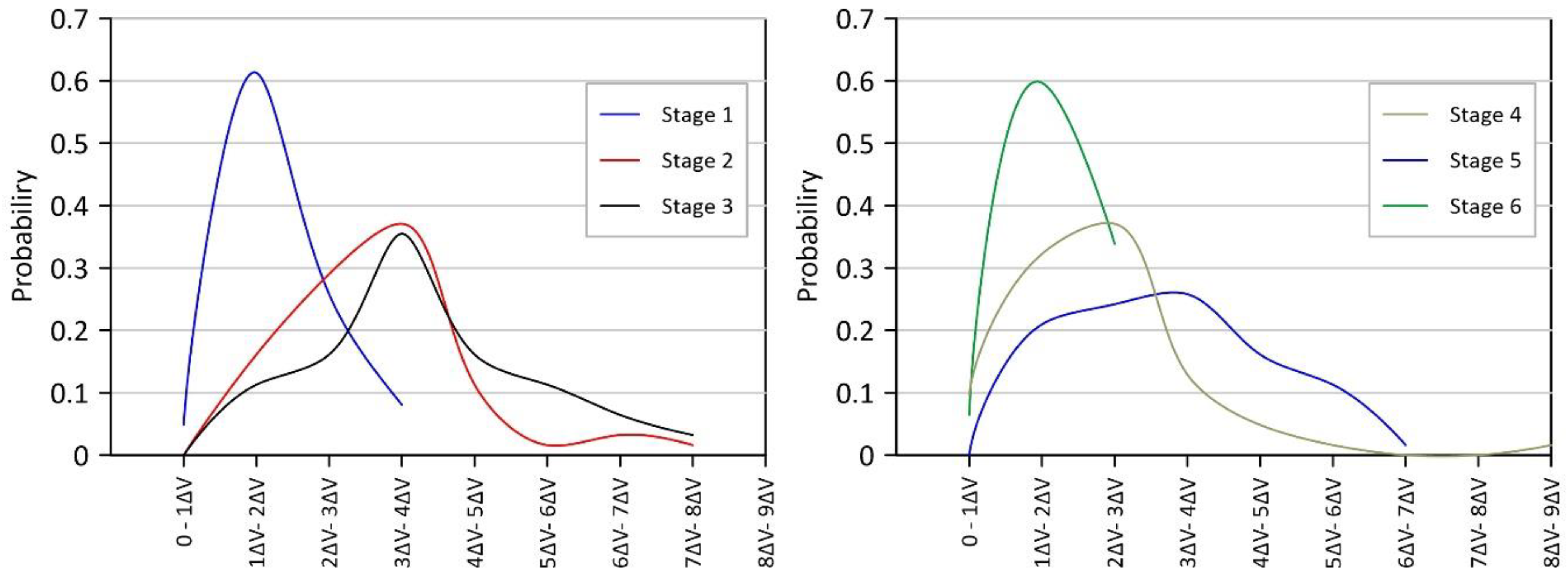
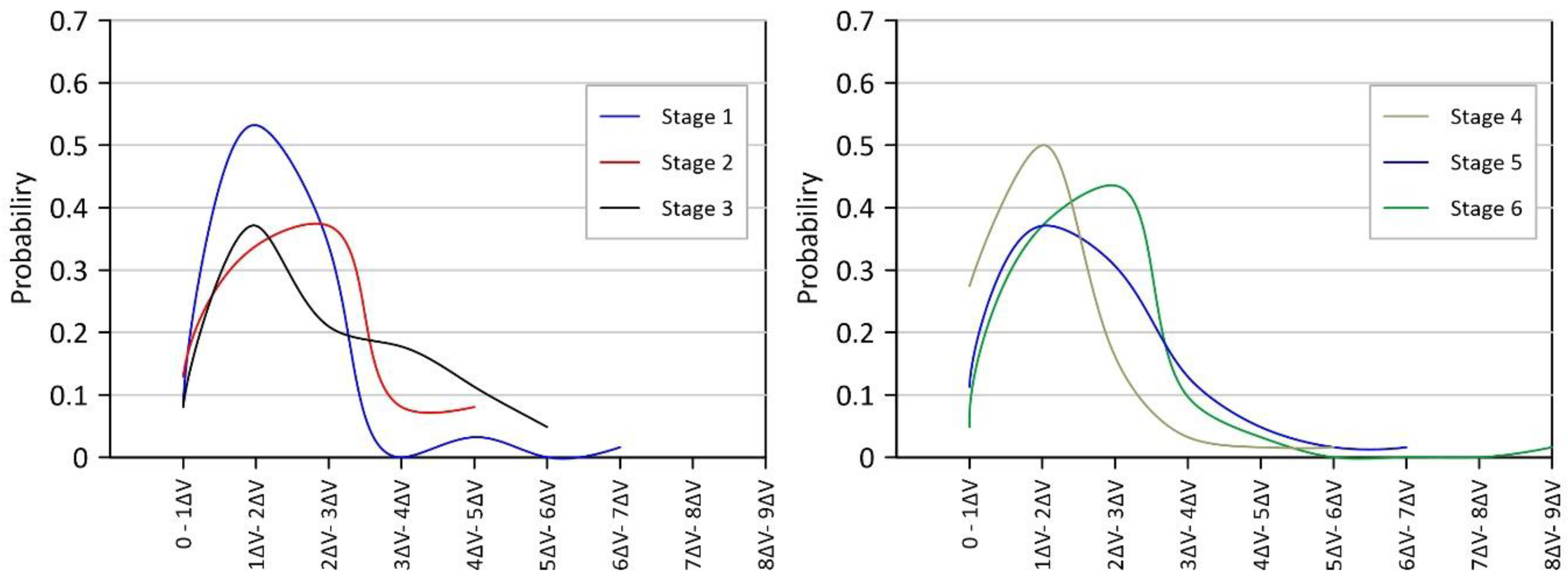
- 4
To take into account the randomness of the inflows, they are defined by a probability density function. In
Figure 4 and
Figure 5 the probabilities (JP in Equation (5)) associated with the historic inflows are given for each stage and each dam.
- 5
For both trials, the discount factor was fixed at 0.5.
- 6
The maximum number of iterations is 100.
- 7
To obtain the solution vectors, i.e., the optimum releases for each stage and each dam, the time was quantified.
Summary 3. Simulation assumptions
Year 1 (1959) has the dams full, with 10,000 hm3 at La Angostura and 7500 hm3 at Malpaso.
The simulation process begins in January, ending in December.
Using the initial storage, the corresponding time, and the file with the optimal release for each time and for each storage level of the reservoirs, the release is obtained.
The operation of the system is based on the principle of continuity, i.e., the new filling level is calculated by adding the inflows and subtracting the releases and other outflows (mainly evaporation) from the initial storage for each time interval.
The storage constraints are evaluated and it is determined whether the system is in a no-spill, spill, or deficit condition with the new storage value.
The process continues until the number of years analysed is reached.
The initial storage, spillage, deficit volumes and average energy generated were analysed. These variables were the evaluation parameters of the optimal policy.
4. Results
4.1. Evaluating the Convergence Criterion
The two trials were performed on a computer with an Intel (R), with a 2.20 GHz processor, 16 GB RAM, and a 64-bit operating system.
Trial 1
- (a)
The optimal policy was obtained when the number of iterations reached its limit (100 in this case); the computation time was 34 s without achieving the convergence criterion (fixed at 0.5 × 10⁻⁴).
- (b)
The differences between each iteration decrease rapidly, but the values oscillate between 10
−2 and 10
−3 from the fifth iteration onwards, thereafter the convergence process is trapped in a loop that repeats values until the maximum number of iterations is reached (
Figure 6).
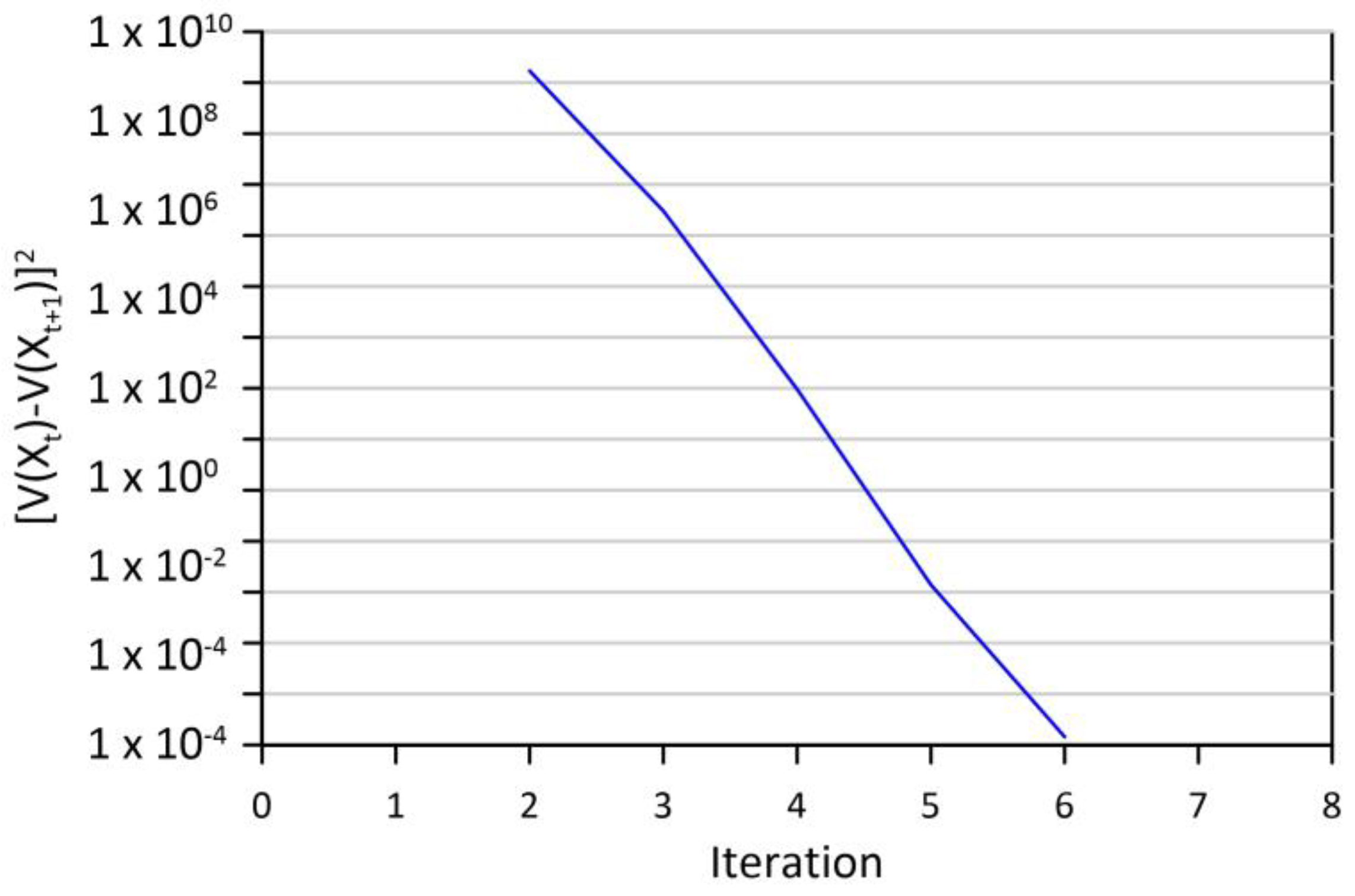
Trial 2
- (a)
The optimal policy was obtained in 5 s, meeting the convergence criterion in the sixth iteration.
Figure 7 shows the details of the iteration cycle.
- (b)
The difference between the first two iterations is significant at the beginning, but it decreases rapidly, and each iteration maintains a negative gradient that leads to finding the optimal policy and concluding the iterative process by meeting the convergence criterion.
Analysing the differences of the solution vectors that give rise to
Figure 6 and
Figure 7, the following can be observed:
- (a)
In both trials the differences are gradually being reduced, towards a solution. However, in trial 1 this trend is seen only until iteration 9; from there, the method falls into a cycle that repeats values systematically, i.e., it reaches a point where it is not possible to improve the solution and the differences between two consecutive iterations do not satisfy the tolerance, without reaching the maximum number of iterations.
- (b)
In trial 2, taking the squared differences amplifies the larger differences between the values of one iteration and the next. However, as these are always decreasing, they are better than those of trial 1, as they are increasingly smaller and thus reach one of the ways of stopping the algorithm, complying with the established tolerance value.
- (c)
The minimum values that trial 1 manages remain in the range of thousandths, while the tolerance was set at a value in the range of ten thousandths. Therefore, here it is worth noting that if the tolerance is relaxed a little, trial 1 would manage to reach this, although trial 2 would be better, as the computational time is less.
A quick trial was designed with new conditions in the optimization process to see what the times would be for the two trials: seven stages were defined, aΔV of 200 hm3 was considered (with this we go from having 22 states in La Angostura to 65 and in Malpaso from 16 to 46), the values for minimum releases were from 3ΔV to 12ΔV in La Angostura= and from 4ΔV to 18ΔV in Malpaso, and maximum releases were 64ΔV for La Angostura and 84ΔV for Malpaso. New data files were prepared and it was found that trial 1 ran for 1 h 12 min 26 s, without managing to meet the tolerance, while trial 2 arrived at a solution in 7 min 40 s, meeting the tolerance at iteration 11.
This trail shows that, if any changes to the system conditions are required to adjust the operating rule, the way the calculation of the differences in the solution vector is set up is extremely important. This quick trial was not carried out as a simulation in this work, but is only given as a reference on how the computational resource demands and execution time grow as the value for discretising the state variables that the dynamic programming algorithm occupies becomes finer and how the criterion for calculating the differences in the solution vector in two consecutive iterations impacts on it.
4.2. Evaluating the System Operation with the Optimal Policy
The optimal policy obtained for each trial was analysed and some differences were found between them, shown in
Figure 8. The results are presented as a state-release matrix for each stage. Each matrix was compared and, if the release was different, then the cell was given a logical value of false (F).
Figure 8 shows that there are only different release values in stages 4 (states 10 in La Angostura and 7 for Malpaso), 5 (states 10 and 6; 11 and 4; 12 and 6; 13 and 5), and 6 (state 20 in La Angostura and from 1 to 16 in Malpaso).
To see if the operating policies of the trials produce significant changes in the behaviour of the system, the historical record of income volumes from 1959 to 2020 was used for the two policies. In general, the simulation process showed:
Similarities between trial 1 and trial 2:
- (a)
The average release per fortnight was 390 hm3 in La Angostura, and 709 hm3 in Malpaso. In both dams, there were events when it was necessary to use the maximum capacity of the turbines, 11 times in La Angostura and only once in Malpaso.
- (b)
In the 62 years simulated, the minimum release at La Angostura dam was 150 hm3, recorded eight times and always occurring in the second half of July. At Malpaso, the minimum release was 300 hm3, occurring 13 times in total: eight times in the first half of November, once in the second half of July, once in the first half of June, once in the second half of June and twice in the second half of May.
- (c)
There are no periods in which the minimum required volume was not satisfied.
- (d)
In only one year, 2010, there was a spill event, occurring at the Malpaso dam. The spill occurred twice: in the last half of September and the first half of October.
- (e)
Both dams maintain average storage levels of a little over half their useful capacity.
Differences between trial 1 and trial 2:
- (a)
For the 62 simulated years, the volumes released in La Angostura were 580,310 hm3 in trial 1, and 580,309 hm3 in trial 2, while in Malpaso these volumes were 1,043,924 hm3 and 1,043,917 hm3, respectively.
- (b)
The only spill event occurred in September/October 2010 at the Malpaso dam, showing only a 2 hm3 difference, 155 hm3 in trial 1, 157 hm3 in trial 2.
- (c)
The average storage volumes for Malpaso dam showed a slight difference: 4991 hm3 in trial 1, and 4997 hm3 in trial 2.
The 4 main variables were evaluated: the minimum value of the initial storage, spillage and deficit volumes, and the average energy. The results are given in
Table 2.
- (a)
The average energy and deficit volume variables remain unchanged in the trials.
- (b)
The minimum storage value reached in each dam is practically the same, with approximately 68 hm3 more in Malpaso between trials 2 and 1; however, this difference is minimal in showing a notable change in the performance of the other variables.
- (c)
In general, the results of the simulation of the operation of the system with the two policies are similar.
4.3. Discussion of Results
The dynamic programming algorithm has been proven to be a robust methodology for application in the study of operating rules for large-capacity storage systems. The case analysed here is of great complexity, as the four reservoirs of the Grijalva river hydroelectric system operate in cascade. In addition, its operation is of great importance nationally, as it is one of the biggest contributors to the generation of electricity. However, the storage levels must be kept within ranges that mean operation is as safe as possible and that extreme weather events do give rise to overflows that cause flooding in downstream populations. It is therefore vital to have tools that allow the testing of different operating conditions, where results are obtained as quickly as possible, to facilitate better management.
From previous works it was seen that the optimization process, in order to obtain the operation rule, often entered a cyclic series, repeating values without achieving satisfaction of the tolerance criterion and always arriving at the maximum number of iterations to stop the process. This led us to focus on how to calculate the differences of the solution vector between two consecutive iterations. A trial was proposed to make this calculation, taking the squared differences (instead of the absolute value), thus magnifying the larger differences, but also flattening the process more rapidly when the differences were small.
With the two trials defined it was seen that the optimal policy of each has few changes and the operation of the system with both is practically the same in the simulation of the system behaviour over the 62 years of historical records used. However, the condition chosen to stabilize the process and achieve convergence has a great impact on the computation time, mainly in the optimization process.
If smaller values are used to discretize the state variables, this will increase the computation time required to find the solution, therefore the choice of the stopping condition is more important, as seen in the results of the quick trial carried out with a finer discretisation interval (aΔV of 200 hm3 instead of 600 hm3), defining one more stage and recalculating the variables involved in the optimisation process by making these changes.
It seems that accumulating the squared differences during a complete cycle (one year) is much better than taking only their absolute value. For the case analyzed, the convergence criterion was met in only six iterations by taking the squared differences, thus avoiding the loop of the first trial. However, it is necessary to test cases that imply a greater demand for computational resources to see if the iterative process is completed by meeting the convergence criterion proposed in this study, and thus avoid the eternal loops inherent in recursive methods.
5. Conclusions
In this paper, two ways to obtain the differences in the solution vector were analysed. They were compared against a defined criterion to achieve convergence and stop the iterative process of the Bellman equations for dynamic stochastic programming. It was seen that taking the squared differences, instead of the absolute value, significantly reduces computation times and the convergence condition is accurately reached.
In future work, we hope to explore the effect of relaxing the tolerance value with the discount factor and to see if this shortens the solution times in more computationally demanding cases. It is also hoped to see if it is still possible to stop the process by satisfying the tolerance criterion, calculating the differences in the solution vector of two consecutive iterations with the square of them.
An advantage of the application reported in this study is that the software does not require large, expensive computer hardware, making it accessible to the federal agencies in charge of managing water storage systems in Mexico.
With the results presented, numerical modelling under similar conditions can be carried out more efficiently, allowing resources to be invested in more comprehensive analyses.
Author Contributions
Conceptualization, R.M.-R.; methodology, R.M.-R.; formal analysis, R.M.-R.; resources, R.S., R.D.-M. and E.C.-E.; data curation, R.M.-R. and R.S.; writing-original draft preparation, R.M.-R. and R.S.; writing-review and editing, R.M.-R., R.S., R.D.-M., E.C.-E. and E.J.-D.; visualization, R.M.-R., R.S., R.D.-M., E.J.-D. and E.C.-E.; supervision, R.M.-R., R.S. and R.D.-M.; funding acquisition, R.D.-M. and E.C.-E. All authors have read and agreed to the published version of the manuscript.
Funding
This research received no external funding.
Data Availability Statement
Not applicable.
Conflicts of Interest
The authors declare no conflict of interest.
References
- Bellman, R.; Kalaba, R. Dynamic programming and statistical communication theory. Proc. Natl. Acad. Sci. USA 1957, 43, 749–751. [Google Scholar] [CrossRef] [PubMed]
- Wu, X.; Cheng, C.; Lund, J.R.; Niu, W.; Miao, S. Stochastic dynamic programming for hydropower reservoir operations with multiple local optima. J. Hydrol. 2018, 564, 712–722. [Google Scholar] [CrossRef]
- Mousavi, S.J.; Ponnambalam, K.; Karray, F. Reservoir Operation Using a Dynamic Programming Fuzzy Rule–Based Approach. Water Resour. Manag. 2005, 19, 655–672. [Google Scholar] [CrossRef]
- Chang, F.-J.; Hui, S.-C.; Chen, Y.-C. Reservoir operation using grey fuzzy stochastic dynamic programming. Hydrol. Process 2002, 16, 2395–2408. [Google Scholar] [CrossRef]
- Raman, H.; Chandramouli, V. Optimal operation of multi-reservoir system using dynamic programming and neural network. WIT Trans. Inf. Commun. Technol. 1996, 16, 11. [Google Scholar]
- Kularathna, M.D.U.P. Application of Dynamic Programming for the Analysis of Complex Water Resources Systems: A Case Study on the Mahaweli River Basin Development in Sri Lanka; Wageningen University and Research: Wageningen, The Netherlands, 1992. [Google Scholar]
- Alaouze, C.M. The Optimality of Capacity Sharing in Stochastic Dynamic Programming Problemas of Shared Reservoir Operation 1. JAWRA J. Am. Water Resour. Assoc. 1991, 27, 381–386. [Google Scholar] [CrossRef]
- de los Reyes, A.G. Improved Stochastic Dynamic Programming for Optimal Reservoir Operation Based on the Asymptotic Convergence of Benefit Differences; University of Arizona: Tucson, AZ, USA, 1974. [Google Scholar]
- Brass, C. Optimising Operations of Reservoir Systems with Stochastic Dynamic Programming (SDP) under Consideration of Changing Objectives and Constraints; Ruhr Universitaet Bochum: Bochum, Germany, 2006. [Google Scholar]
- Lim, D.-G.; Kim, J.-H.; Kim, S.-K. A Stochastic Dynamic Programming Model to Derive Monthly Operating Policy of a Multi-Reservoir System. Korean Manag. Sci. Rev. 2012, 29, 1–14. [Google Scholar] [CrossRef]
- Macián Sorribes, H. Design of Optimal Reservoir Operating Rules in Large Water Resources Systems Combining Stochastic Programming, Fuzzy Logic and Expert Criteria; Universitat Politècnica de València: Valencia, Spain, 2017. [Google Scholar]
- Rougé, C.; Tilmant, A. Using stochastic dual dynamic programming in problems with multiple near-optimal solutions. Water Resour. Res. 2016, 52, 4151–4163. [Google Scholar] [CrossRef]
- Al-MohseenA, K.; Tawfiiq, A. Stochastic Dynamic Programming Model for Single Reservoir. AL-Rafidain Eng. J. (AREJ) 2014, 22, 1–14. [Google Scholar]
- Gjerden, K.S.; Helseth, A.; Mo, B.; Warland, G. Hydrothermal scheduling in Norway using stochastic dual dynamic programming; a large-scale case study. In Proceedings of the 2015 IEEE Eindhoven PowerTech, Eindhoven, The Netherlands, 29 June–2 July 2015; pp. 1–6. [Google Scholar]
- Leclère, V.; Carpentier, P.; Chancelier, J.-P.; Lenoir, A.; Pacaud, F. Exact Converging Bounds for Stochastic Dual Dynamic Programming via Fenchel Duality. SIAM J. Optim. 2020, 30, 1223–1250. [Google Scholar] [CrossRef]
- Khan, K.; Goodridge, W. Stochastic Dynamic Programming in DASH. Int. J. Adv. Netw. Appl. 2019, 11, 4263–4269. [Google Scholar] [CrossRef]
- Brandi, R.B.S.; Marcato, A.L.M.; Dias, B.H.; Ramos, T.P.; Junior, I.C.d.S. A Convergence Criterion for Stochastic Dual Dynamic Programming: Application to the Long-Term Operation Planning Problem. IEEE Trans. Power Syst. 2018, 33, 3678–3690. [Google Scholar] [CrossRef]
- Marescot, L.; Chapron, G.; Chadès, I.; Fackler, P.L.; Duchamp, C.; Marboutin, E.; Gimenez, O. Complex decisions made simple: A primer on stochastic dynamic programming. Methods Ecol. Evol. 2013, 4, 872–884. [Google Scholar] [CrossRef]
- Stedinger, J.R.; Sule, B.F.; Loucks, D.P. Stochastic dynamic programming models for reservoir operation optimization. Water Resour. Res. 1984, 20, 1499–1505. [Google Scholar] [CrossRef]
- Langen, H.-J. Convergence of Dynamic Programming Models. Math. Oper. Res. 1981, 6, 493–512. [Google Scholar] [CrossRef]
- Homem-de-Mello, T.; de Matos, V.L.; Finardi, E.C. Sampling strategies and stopping criteria for stochastic dual dynamic programming: A case study in long-term hydrothermal scheduling. Energy Syst. 2011, 2, 1–31. [Google Scholar] [CrossRef]
- Jaakkola, T.; Jordan, M.; Singh, S. Convergence of stochastic iterative dynamic programming algorithms. Adv. Neural Inf. Processing Syst. 1993, 6, 703–710. [Google Scholar]
- Hooshyar, M.; Mousavi, S.J.; Mahootchi, M.; Ponnambalam, K. Aggregation–Decomposition-Based Multi-Agent Reinforcement Learning for Multi-Reservoir Operations Optimization. Water 2020, 12, 2688. [Google Scholar] [CrossRef]
- Mendoza, R.; Arganis, M.; Domínguez, R. Políticas de operación con variación temporal en los coeficientes de castigo de las curvas guía en un sistema multiembalse. In Proceedings of the XXV Congreso Nacional de Hidráulica, Mexico City, México, 5–9 November 2018. [Google Scholar]
- Mendoza, R.; Domínguez, R.; Arganis, M. Influencia de curvas guía en las políticas de operación para el manejo de un sistema hidroeléctrico. In Proceedings of the XXV Congreso Latinoamericano de Hidráulica, San José, Costa Rica, 9–12 September 2012. [Google Scholar]
- Bellman, R. Dynamic Programming; Princeton University Press: Princeton, NJ, USA, 1957. [Google Scholar]
- Mamani, A.A.L. Un Método Recursivo Para el Problema de la Programación Lineal Dinámica; Universidad Nacional San Agustin de Arequipa: Arequipa, Perú, 2018. [Google Scholar]
- Mendoza, R.; Domínguez, R.; Arganis, M. Políticas de operación del sistema hidroeléctrico del río Grijalva considerando el efecto de la correlación en los volúmenes de ingreso. In Proceedings of the XXIII Congreso Nacional de Hidráulica, Puerto Vallarta, Jalisco, México, 15–17 October 2014. [Google Scholar]
- Alayo, H. Introducción a la Programación Dinámica Estocástica. Available online: https://hansroom17.files.wordpress.com/2016/12/dp.pdf (accessed on 1 June 2022).
- Domínguez-Mora, R. Metodología de Selección de Una Política de Operación Conjunta de Una Presa y Su Vertedor; Universidad Nacional Autónoma de México: Mexico City, Mexico, 1989. [Google Scholar]
- Larson, R.E.; Casti, J.L. Principles of Dynamic Programming: Advanced Theory and Applications; Marcel Dekker, Inc.: New York, NY, USA, 1982. [Google Scholar]
- Nandalal, K.; Bogardi, J.J. Dynamic Programming Based Operation of Reservoirs: Applicability and Limits; Cambridge University Press: Cambridge, UK, 2007. [Google Scholar]
- Boutilier, C.; Dearden, R.; Goldszmidt, M. Stochastic dynamic programming with factored representations. Artif. Intell. 2000, 121, 49–107. [Google Scholar] [CrossRef] [Green Version]
- OMM/GWP. Gestión Integrada de Crecientes. Caso de Estudio México: Río Grijalva. Programa Asociado de Gestión de Crecientes. Unidad de Apoyo Técnico. Available online: http://www.floodmanagement.info/publications/casestudies/cs_mexico_full.pdf (accessed on 28 June 2022).
- Juan, E. Elaboración de Mapas Para la Cuenca del Rio Grijalva. Informe Interno. Internal Report. Restricted Circulation.; Instituto de Ingeniería, UNAM: Mexico City, Mexico, 2022. [Google Scholar]
- INECC. La Cuenca de Los Ríos Grijalva y Usumacinta. Available online: http://www2.inecc.gob.mx/publicaciones2/libros/402/cuencas.html (accessed on 28 June 2022).
| Publisher’s Note: MDPI stays neutral with regard to jurisdictional claims in published maps and institutional affiliations. |
© 2022 by the authors. Licensee MDPI, Basel, Switzerland. This article is an open access article distributed under the terms and conditions of the Creative Commons Attribution (CC BY) license (https://creativecommons.org/licenses/by/4.0/).

 ,
, 


