
Unsupervised Representation Learning of GRACE Improves Groundwater Predictions

Lexington High School, 251 Waltham St, Lexington, MA 02421, USA
Water 2022, 14(19), 2947; https://doi.org/10.3390/w14192947
Submission received: 25 August 2022
/
Revised: 16 September 2022
/
Accepted: 16 September 2022
/
Published: 20 September 2022
(This article belongs to the Special Issue AI and Deep Learning Applications for Water Management)
Abstract
:Groundwater is a crucial source of the world’s drinking and irrigation water. Nonetheless, it is being rapidly depleted in many parts of the world. To enact policy decisions to preserve this precious resource, policymakers need real-time data on the groundwater levels in their local area. However, groundwater monitoring wells are costly and scarce in supply. The use of satellite imagery is a promising alternative with its ability to provide continuous information over a large area. Machine learning has also emerged as an alternative to computationally intensive physics-based models. However, advancements in machine learning such as unsupervised learning methods have never been translated to groundwater modeling. Thus, in this paper, learned representations were generated for the GRACE satellite for the first time. When used as an input to groundwater prediction models, the learned representations reduce the root mean square error (RMSE) by up to 19% and improve the Nash–Sutcliffe efficiency (NSE) by up to 8x compared to traditional satellite data inputs at three different spatial scales: national, state, and county. The learned representations are able to discern fine-grained patterns from the coarse satellite data, globally downscaling the GRACE satellite. Crucially, the globally trained representations have the potential to improve the performance of virtually every machine learning-based groundwater prediction model. With accurate measurements, local officials are empowered to make proactive decisions to ensure the stability of their region’s water.
1. Introduction
Groundwater management is crucial for maintaining the world’s water resources. Fifty percent of the world relies on groundwater for drinking, and forty-three percent relies on groundwater for irrigation [1]. Factors such as over-pumping, climate change, and poor management are placing increasing stress on groundwater resources [2,3]. Policy decisions to preserve this precious resource require timely up-to-date information on the current status of groundwater [4]. Without continuous information, local officials can be unaware of changes in groundwater, leading to potentially significant damages to the resource [5].
However, current groundwater monitoring networks are not able to provide this crucial information. Dedicated monitoring wells are necessary for high-quality groundwater information, but they are expensive. Building high-quality monitoring wells can cost between $100,000 and $200,000 per well [6]. Thus, these wells are few and far between. The need for a scalable groundwater modeling framework to augment physical monitoring wells is evident. Remote sensing, with its ability to extract detailed global information in real time, is a low-cost alternative that has shown promise in the literature.
The leading satellites for measuring global trends in water storage are Gravity Recovery and Climate Experiment (GRACE) and its successor, Gravity Recovery and Climate Experiment Follow-On. However, the GRACE satellites have a coarse spatial resolution of 200,000 km2, making them sensitive only to large-scale changes in water mass. Because the GRACE data only provides a singular terrestrial water storage value for an entire 1 × 1 region, it does not capture the variability in groundwater that occurs at the local level. GRACE fails to provide groundwater indicators at a local scale, which is the level at which water management information is the most needed [7]. In order to prevent groundwater stress, management agencies need to know the groundwater trends in their specific watershed so they can be proactive in their policies. If groundwater stress is identified, policies such as managed aquifer recharge (MAR) can be implemented to increase groundwater levels. MAR policies range from implementing infiltration ponds to stream bed channel modifications [8]. However, MAR can only be implemented when there is sufficient information on the current state of groundwater locally.
A prominent focus of the literature is the use of both physical and statistical modeling to predict groundwater metrics using GRACE.
Physics-based modeling has been used for large-scale prediction models. Dynamic models, when forced with meteorological data, can provide approximate representations of interactions between climatic variables and their effects on groundwater. However, physical models pose certain drawbacks as they are computationally intensive [9], and they sometimes do not account for anthropogenic influence. Two prominent examples are Schumacher et al. [10] and Li et al. [11]. The former assimilates GRACE data into the WaterGAP Global Hydrology Model to simulate groundwater storage in the Murray–Darling Basin. They find that parameter calibration and assimilation with GRACE data lead to increased model accuracy. Li et al. use GRACE data as an input to the Catchment Land Surface Model (CLSM), which simulates changes in groundwater levels. Although the predictions are global, the model fails to take into account changes in groundwater levels due to irrigation as CLSM does not simulate this. However, overpumping of groundwater due to irrigation is one of the largest sources of variability in groundwater levels. Specifically, over 20 of the world’s aquifers are being overexploited due to pumping [12]. These drawbacks of physics-based modeling have led the literature to largely focus on machine learning techniques.
These machine learning techniques tend to be small-scale and/or require 10–12 years of time series data in order to generate accurate monthly predictions [13]. For example, Ali et al. [14] use the extreme gradient boosting model to downscale GRACE to a resolution of 0.25 × 0.25 in the Indus Basin Irrigation System. GRACE data, meteorological data such as temperature and precipitation, and elevation data were fed into the downscaling model and validated on ground truth data. While the model achieves strong performance, it is limited to only a singular basin. Thus, acquiring predictions for multiple basins would require retraining the model with data from each basin. This method does not generalize to areas where there are limited monitoring data [15]. Studies have also downscaled GRACE using time-series data. Gorugantula and Kambhammettu [16] use a long short-term memory network to spatially downscale GRACE data in the Krishna River basin. Similar to other downscaling studies, they augment GRACE data with meteorological variables and face drawbacks due to their limited area of study. In addition, the quality of downscaling is directly dependent on the amount of time-series data available. Applying this framework to the many regions with limited availability of time-series data would result in a poor downscaling of GRACE.
Ultimately, while the methods described above achieve acceptable performance in groundwater prediction, there is significant room for improvement [17]. Despite the abundance of downscaling studies, the main drawback remains the coarse resolution of GRACE. This has yet to be solved on a large scale.
Previous work is able to downscale GRACE through supervised learning. However, the novelty of this paper is that it uses unsupervised representation learning to downscale GRACE. Unsupervised learning does not require ground-truth well values. Thus, it is possible to generate informative representations of the GRACE satellite that are globally applicable.
In addition, it is to be noted that this method is not at odds with any of the methods discussed above. Any machine learning model can use the representations as input instead of raw satellite data, leading to an immediate performance boost. Because the representations are globally applicable, they are downscaling GRACE on a large scale.
An unsupervised learning method was developed by taking inspiration from the field of natural language processing (NLP). The Word2Vec [18] model has proven to be enormously useful for NLP prediction tasks [19]. This model learns a vector representation of a word via an unsupervised learning task to predict the word given its surrounding words. This vector represents the rich, semantic meaning of the word. Semantically similar words’ corresponding vectors have a small Euclidean distance, for example.
This paper applies a similar methodology to learn informative representations of the GRACE satellite. Similar to how Word2Vec capitalizes on the semantic meaning of words, the inherent spatiotemporal correlation of satellite data can also be capitalized on. The representation learning model learns to extract these correlations and translate them to a vector. This vector thus captures the important patterns better than the raw data itself, leading to improved performance on downstream tasks.
Previous implementations of unsupervised representation learning in remote sensing have been limited despite the significant gains provided in other fields. One of the only examples is Agastya et al. [20], who use the SimCLR framework to generate learned representations for Sentinel 2 satellite data. The model takes in an image and passes it through a convolutional neural network and then a multilayer perceptron. The objective ensures that the output of the perceptron is similar for random crops from the same image and different if the crops are from different images. The learned representations were found to significantly increase accuracy for downstream tasks, specifically, 9x precision and 90% better recall on irrigation detection.
Unsupervised representation learning is uniquely poised to address groundwater modeling’s biggest problem: the low resolution of GRACE. To implement unsupervised representation learning for GRACE satellite data, a neural network model was trained on GRACE and other meteorological satellites. The model is able to use the other meteorological measurements to learn a spatiotemporal representation of the GRACE data, essentially “downscaling” GRACE. By learning the underlying correlations between the satellite data, the resulting learned representation vector can better represent groundwater indicators at a specific location. When these representations are used as an input to a machine learning groundwater prediction model, they reduce error by up to 19% compared to raw satellite data. The globally trained representation learning model provides learned representations that can be used for virtually every machine learning groundwater prediction task. By increasing the accuracy of groundwater predictions, local officials are provided with the detailed information necessary to manage groundwater resources.
2. Materials and Methods
2.1. Model Framework
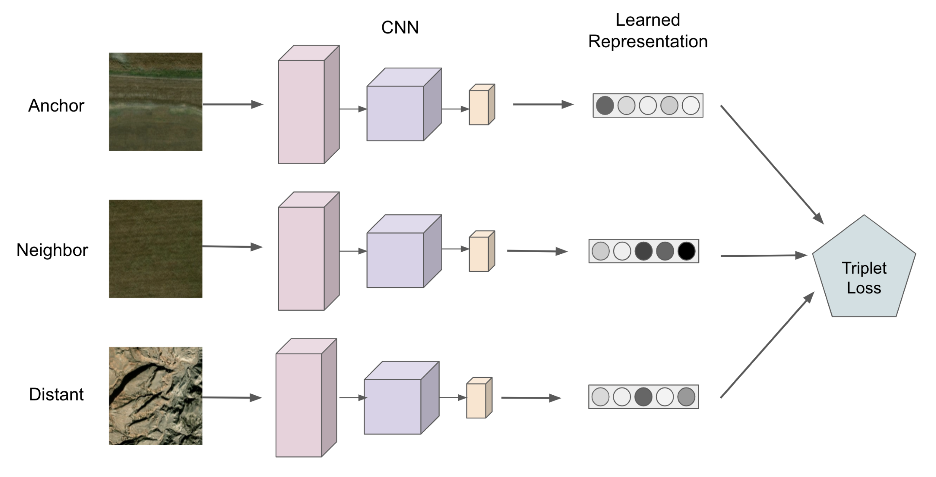
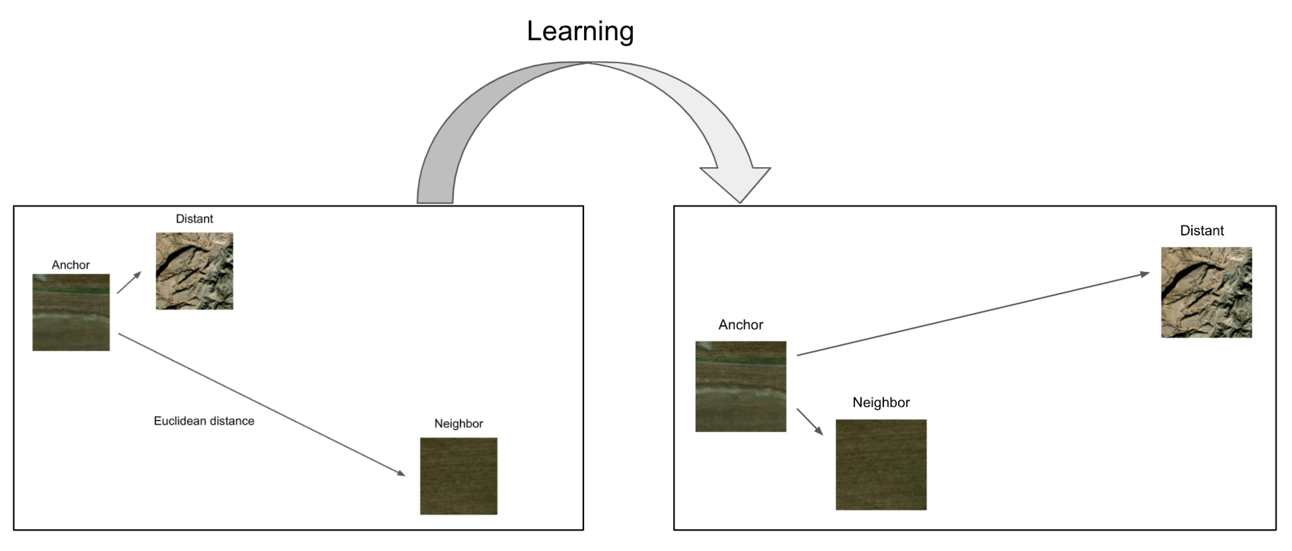
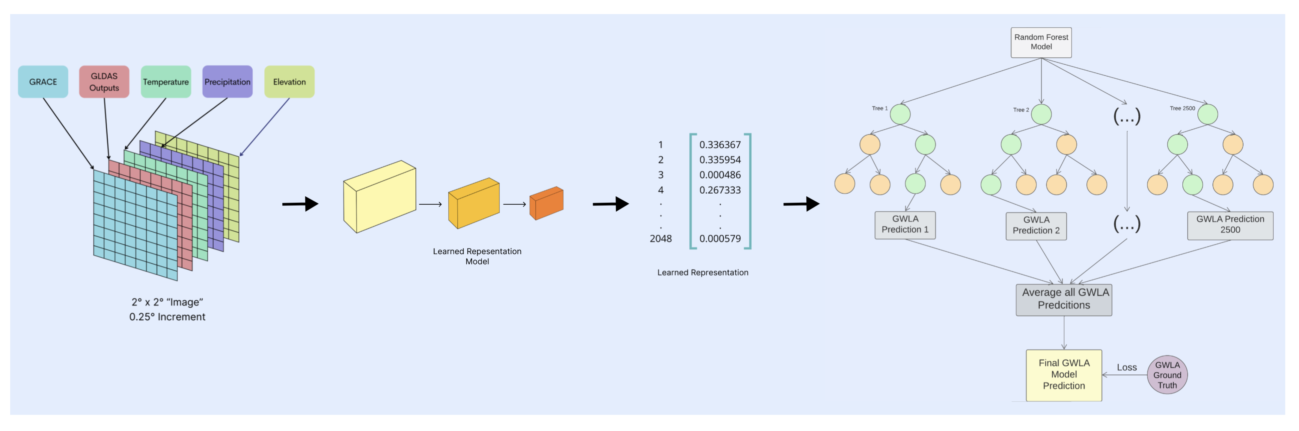
The Tile2Vec model [21] is used to develop representations of the satellite data. The Tile2Vec model uses a state-of-the-art convolutional neural network (CNN) for unsupervised representation learning of spatially distributed data. CNNs are used because of their success in image classification tasks. CNNs can quickly extract “features” from the image using convolutional filters. Thus, the CNN is well suited to extract spatial correlations in the satellite data. This process is depicted in Figure 1. The CNN is fed three satellite data images. The first image is an anchor image. The second image is a neighbor image that is spatially adjacent to the anchor image. The third image is a distant image that is spatially distant to the anchor image. Through unsupervised triplet loss, the CNN is trained to minimize the Euclidean distance between the learned representations of the anchor image and the neighbor image and maximize the Euclidean distance between the learned representations of the anchor image and distant image, as shown below in Figure 2. By capitalizing on spatial correlations, the model is able to learn meaningful representations of the satellite data across space and time. In addition, an L2 weight regularization term is added to the loss. A margin term in the loss prevents the model from continually pushing apart distant images; a Euclidean distance greater than the margin will not decrease the loss. The output of the model is a 2048-long vector that acts as a semantically significant distillation of the satellite image.
2.2. Model Inputs
The Tile2Vec model is trained on multiple remotely sensed datasets, including GRACE, precipitation, temperature, and Global Land Data Assimilation System outputs. Because GRACE’s data are quite coarse, the addition of multiple features helps the Tile2Vec model interpolate between data points.
Model inputs are summarized below and in Table 1.
2.2.1. GRACE TWS
GRACE TWS for the GRACE and GRACE-FO satellites were obtained with the GRACE JPL-RL06M mascons solution from the Jet Propulsion Laboratory. Data are available at a spatial resolution of 0.1 × 0.1 from 2002 to 2021 with the exception of mid-2017 to mid-2018. Data were downloaded from the NASA PO.DAAC Drive.
2.2.2. Precipitation
Precipitation data were obtained from NASA Global Precipitation Measurement through the NASA GES DISC. The GPM (IMERG) product provides monthly global precipitation from 2000 to 2021 at a spatial resolution of 0.1 × 0.1 (URL: https://disc.gsfc.nasa.gov/datasets/GPM_3IMERGM_06/summary; access date: 16 April 2022).
2.2.3. Temperature
Land surface temperature data were obtained from the MERRA-2 product through NASA GES DISC. MERRA-2 provides monthly global temperatures from 1980 to 2021 at a spatial resolution of 0.5 × 0.625 (URL: https://daac.gsfc.nasa.gov/datasets/M2TMNXSLV_5.12.4/summary; access date: 18 April 2022).
2.2.4. GLDAS Outputs
Outputs from the Global Land Data Assimilation System (GLDAS) NOAH 2.1 Land surface model were used, namely, Wind Speed, Evapotranspiration, Root zone soil moisture, Baseflow groundwater runoff, Plant canopy surface water, Snow water equivalent, Storm surface runoff, and Soil moisture, at a spatial resolution of 0.25 × 0.25. GLDAS simulates hydrological variables by integrating satellite and ground-based observations into land models. Data are available globally (90.0 N to 60.0 S) from 2000 to 2021 (URL: https://disc.gsfc.nasa.gov/datasets/GLDAS_NOAH025_M_2.1/summary; access date: 10 May 2022).
2.2.5. GLDAS Elevation
Elevation data were obtained from the GLDAS elevation field. The data are averaged from the GTOPO30 Global 30 Arc Second (1 km) Elevation Dataset to a resolution of 0.25 × 0.25 (URL: https://ldas.gsfc.nasa.gov/gldas/elevation#:~:text=The%20GLDAS%20elevation%20field%20is,0.25%20degree%20and%201%20degree.; access date: 28 May 2022).
2.3. Model Training
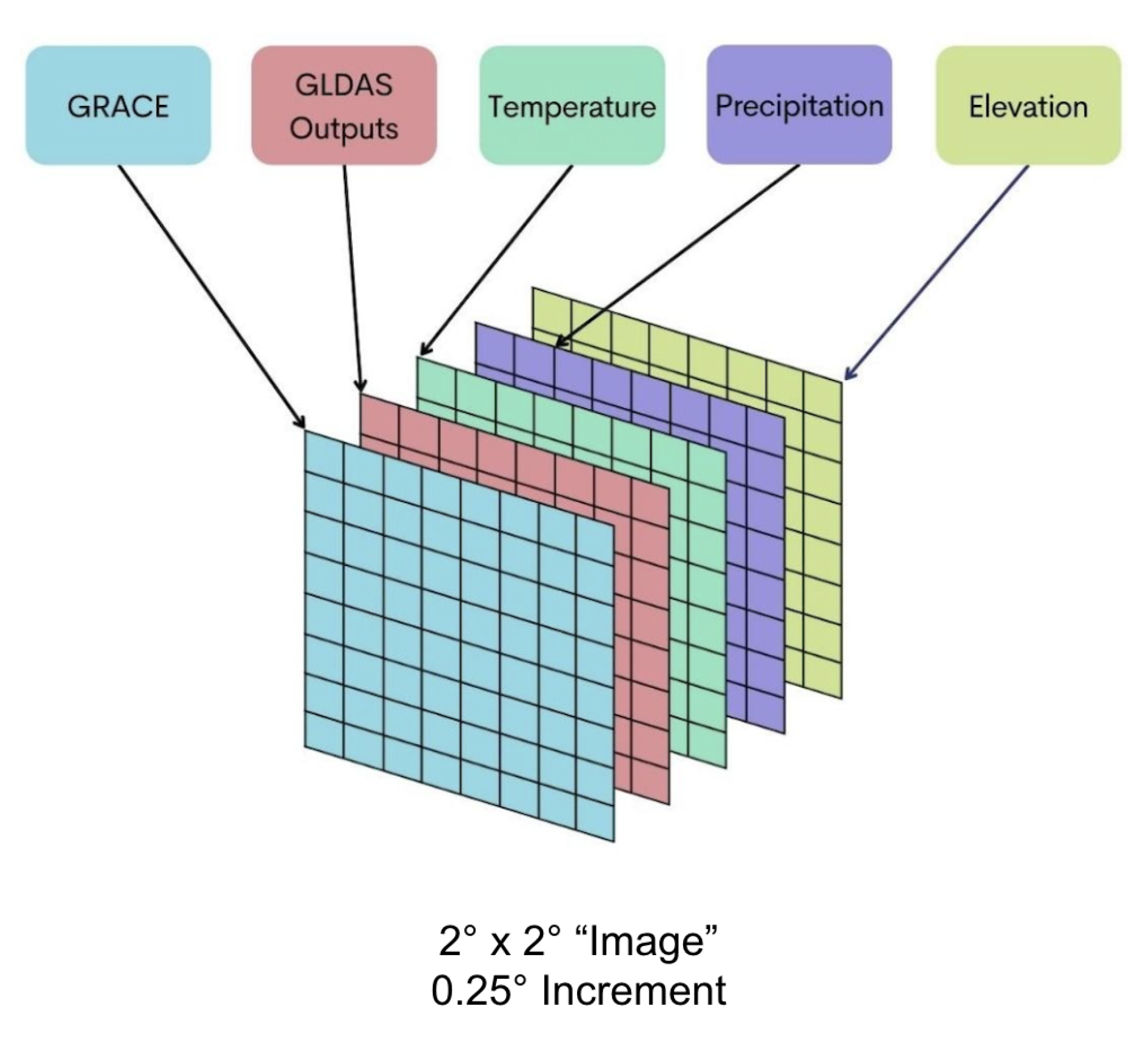
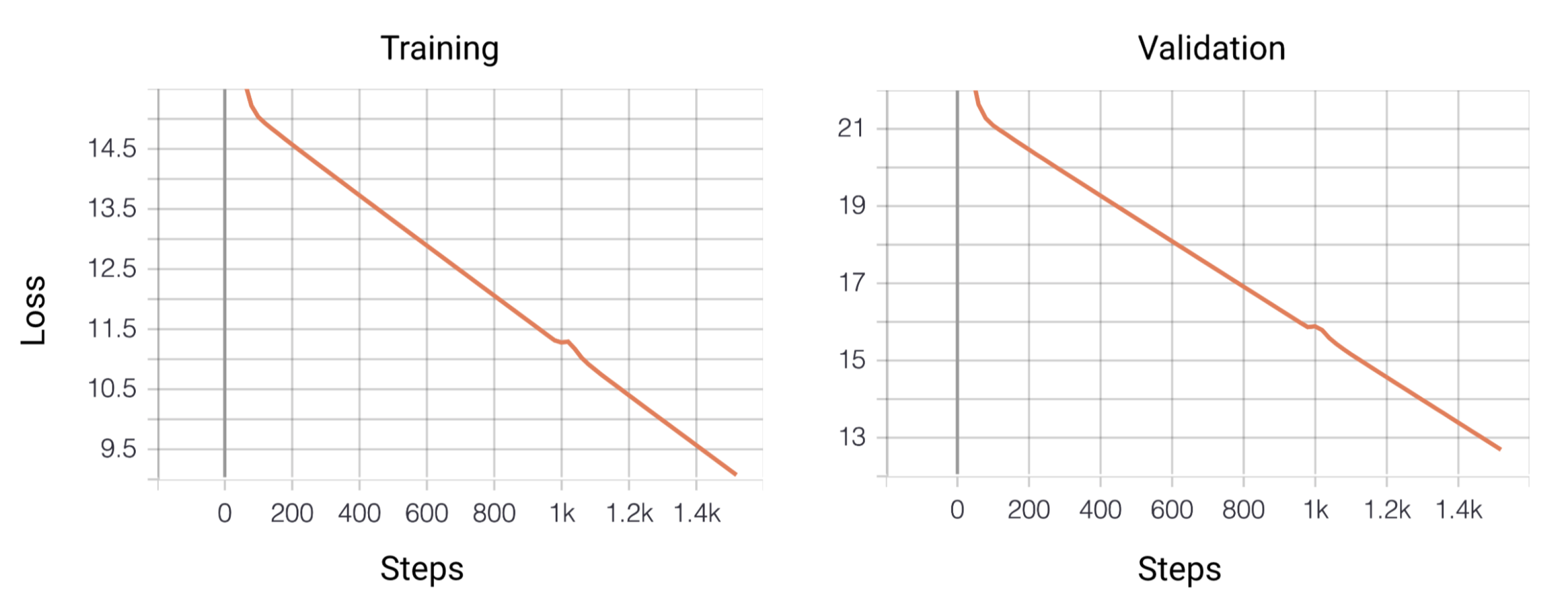
The model takes an “image” as input. An “image” consists of a 2 × 2 coordinate box, with a 0.25 increment, resulting in an 8 × 8 box of coordinates. The GRACE satellite data are at a 1 spatial resolution, whereas much of the other satellite data have a resolution of 0.25. Thus, a 0.25 increment was chosen. Additionally, an 8 × 8 box was chosen as it represents approximately 70,000 km, which is an area that is large enough to capture variability while still being spatially similar to the neighbor image. For each of the coordinates in the image, the 13 satellite data features are queried, acting as the “bands”. This is shown below in Figure 3. The Tile2Vec model was trained on global satellite data. The anchor image is built around a randomly selected point. The neighbor image is built around a point randomly selected on the circumference of a circle with a radius of 3 from the anchor point. The distant image is independently built from a randomly selected point. Images were rejected if they fell on a body of water. This was determined by using the global-land-mask python package. Images were also dropped if they contained any masked values. The Tile2Vec model was trained for 75 epochs with a learning rate of 0.0001 and 20.6 million parameters on one GPU. The batch size was 10,000 images. The loss is an unsupervised triplet loss, as described in Section 2.1. Model training and validation loss curves can be seen in Figure 4.
3. Model Evaluation
The performance of the Tile2Vec learned representations were evaluated at three different spatial scales: national, state, and county, against the raw satellite data baseline. At each level, two random forest models were trained. The objective of both models is to predict groundwater levels. The first random forest model takes in the learned representations as input, and the second takes in the raw satellite data as input. This is shown in Figure 5. All random forest models were trained with 2500 trees and an 80/20 train–test split. All random forest models were validated on ground truth data. Ground truth data were obtained as a depth to water level below surface value. To calculate the change in groundwater level, the data were subtracted from the long-term mean of the site. The long-term mean was calculated by averaging measurements from 2004 to 2009. This is reflective of how GRACE TWS anomalies are calculated, by subtracting from the 2004 to 2009 long-term mean from the current value [22]. By evaluating the Tile2Vec model on multiple spatial scales, it can be seen how the learned representations contribute to the generalizability and accuracy of the models.
3.1. National Model
A national model was trained to predict changes in groundwater levels in the contiguous United States. The U.S. contains great geographical diversity. Its topography includes coastal plains, mountains, temperate and subtropical forests, and grasslands. The long-term average annual precipitation is 76.05 cm, and the long-term mean, minimum, and maximum annual temperatures are 11.83 C, 5.78 C, and 19.06 C, respectively.
Due to irrigation and excess pumping, many regions of the U.S. are currently facing groundwater depletion. Over two out of every three gallons of groundwater is used for irrigation [23]. In some regions in the Central Valley, groundwater overdraft is over 2 million acre-feet annually. The Ogallala Aquifer, one of the world’s largest groundwater resources, is also being rapidly depleted. Between 1900 and 2008, 89 trillion gallons of water have been drained from the aquifer [24]. It is estimated that within the next 50 years, 70% of the entire aquifer will be depleted [25]. With this precious resource rapidly fading, it is crucial that steps are taken to prevent further loss.
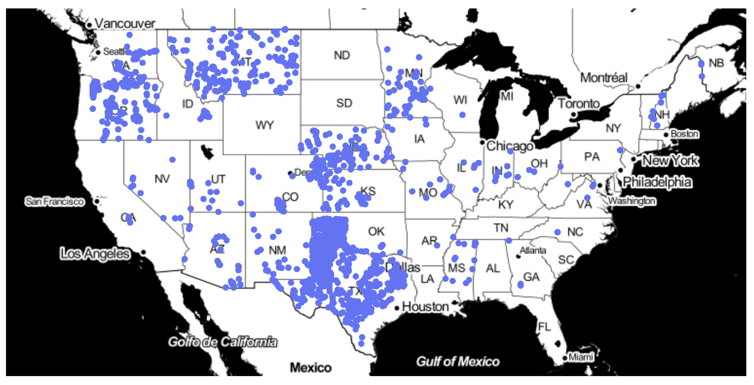
Ground truth well measurement data were obtained from USGS (https://cida.usgs.gov/ngwmn/index.jsp; access date: 11 February 2022). A total of 61,968 data points were obtained for this model. The distribution of the points is shown below in Figure 6.
3.2. State Model
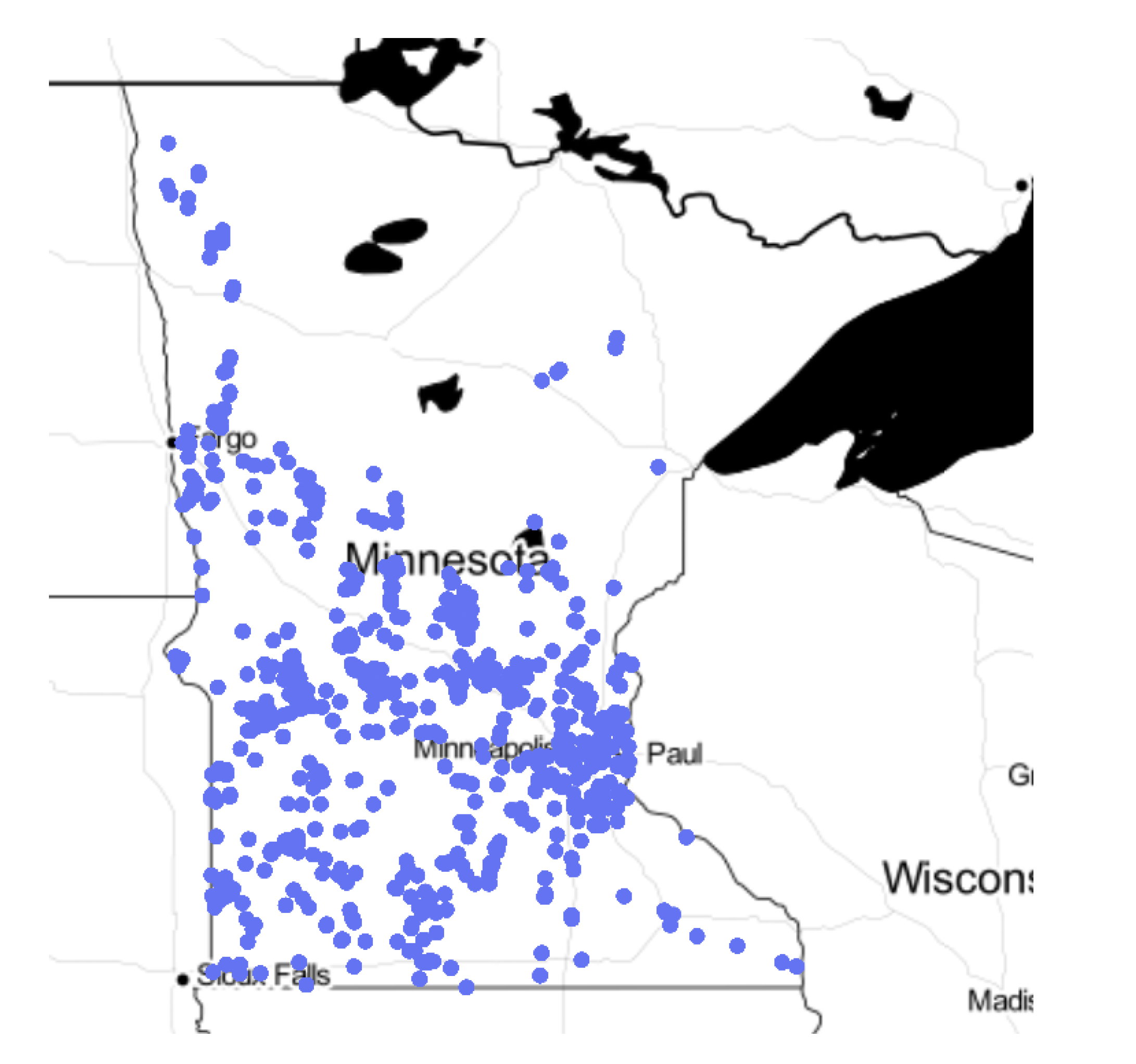
A state-level model was trained to predict changes in groundwater levels for Minnesota. Minnesota experiences a continental climate with below-freezing temperatures in the winter and warm summers. Groundwater accounts for 75% of drinking water and 90% of irrigation water [26]. Central Minnesota has ample groundwater supply, while the northeast and southeast regions face increased stress. Ground truth well measurement data were obtained from the Minnesota DNR (https://www.dnr.state.mn.us/waters/cgm/index.html; access date: 21 February 2022). A total of 69,605 data points were obtained for this model. The distribution of the points is shown below in Figure 7.
3.3. County Model
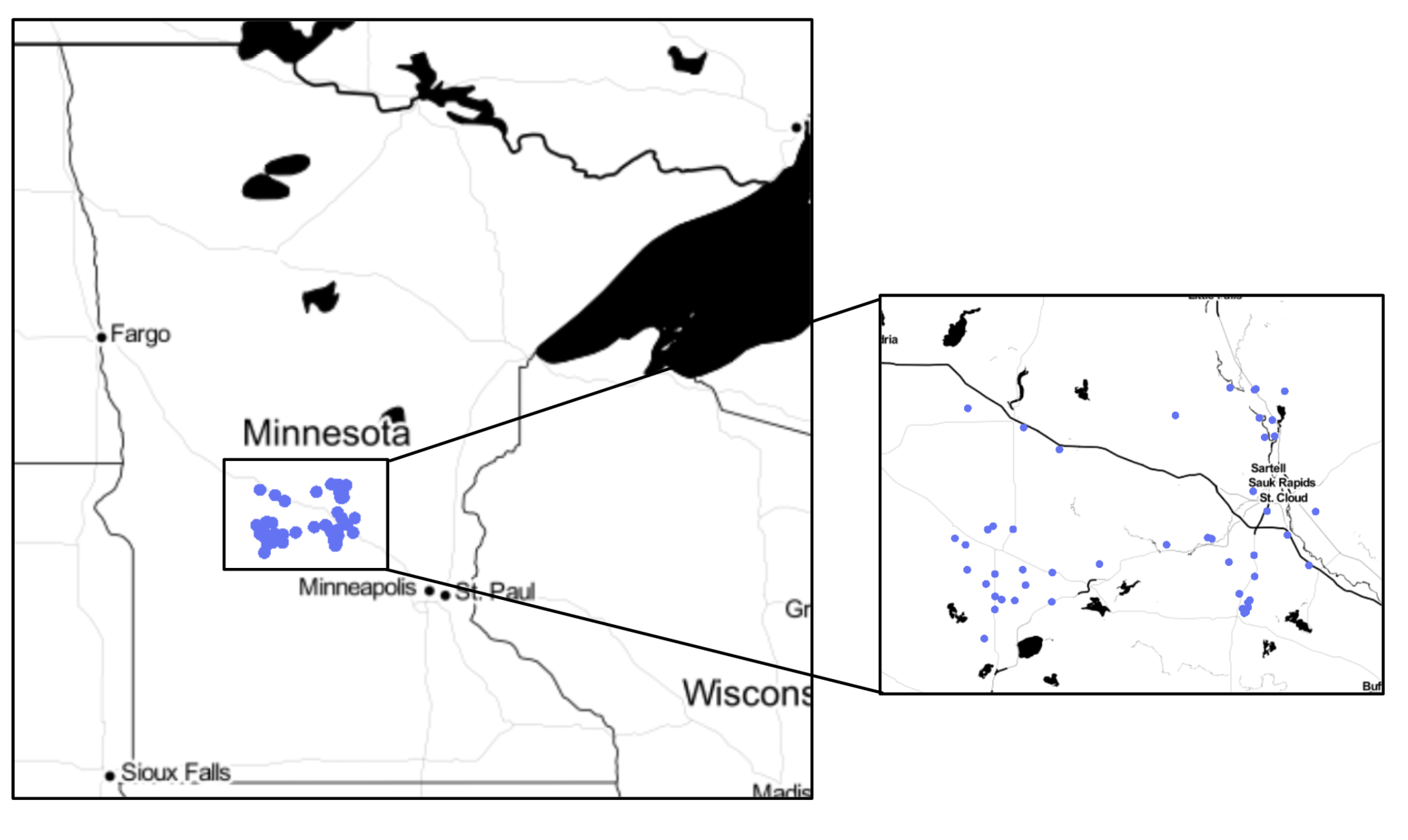
A state-level model was trained to predict changes in groundwater levels for Stearns County, Minnesota. Stearns County is located in central Minnesota. Ground truth well measurement data were obtained from the Minnesota DNR (https://www.dnr.state.mn.us/waters/cgm/index.html; access date: 21 February 2022). A total of 5,802 data points were obtained for this model. The distribution of the points is shown below in Figure 8.
3.4. Error Analysis Metrics
Five metrics were used to analyze the errors and evaluate the performance of the various models on the test set. The metrics are mean absolute error (MAE), correlation coefficient (R), Nash–Sutcliffe efficiency (NSE), Spearman Rho, and root mean square error (RMSE). These metrics are explained below.
3.4.1. Mean Absolute Error (MAE)
The MAE represents the mean of the absolute value of the predicted minus observed values from the data. The closer the MAE is to 0, the lower the model’s error. The equation to calculate MAE is shown below.
3.4.2. Correlation Coefficient (R)
The correlation coefficient represents the measure of which two variables are linearly correlated or changes in one variable account for changes in the other. The closer the absolute value of the coefficient is to 1, the stronger the relationship. The equation to calculate the correlation coefficient is shown below.
3.4.3. Nash–Sutcliffe efficiency (NSE)
The Nash–Sutcliffe efficiency coefficient is used to assess the performance of hydrological models. NSE values range from -∞ to 1. The closer the value to one, the better the predictive power of the model. Generally, values between 0 and 1 are considered acceptable. The equation to calculate the NSE is shown below.
3.4.4. Spearman Rho
The Spearman Rho correlation coefficient is used to assess how well two variables follow a monotonic function. Spearman Rho correlation values range from −1 to 1. The closer the value is to +1 or −1, the stronger the relationship between the two variables. The equation to calculate the Spearman Rho is shown below.
3.4.5. Root Mean Square Error (RMSE)
RMSE represents the standard deviation of the difference between predicted and observed values (residuals). The lower the RMSE, the lower the model’s error. The equation to calculate RMSE is shown below.
4. Results
A summary of results from the three models can be seen in Table 2. The learned representation model consistently performs better than the satellite data model. In the national model, the learned representations provide a 19% improvement in RMSE and a 1.4x improvement in NSE. In the state model, the learned representations provide a 14% improvement in RMSE and a 7.9x improvement in NSE. In the county model, the learned representations provide a 6% improvement in RMSE and a 2.5x improvement in correlation. Across a variety of metrics, it is clear that the learned representations are able to improve performance.
Acceptable performance is achieved in NSE, as all values are greater than 0. Model performance on the NSE and correlation is comparable to that of Miro and Famiglietti [27], who downscale GRACE in Central Valley, California. Miro and Famiglietti test their model on in situ groundwater data and kriged groundwater data. As the data used in this paper were not spatially interpolated, results are compared only on in situ data.
In the above experimental setup, the model must predict groundwater levels for locations and climates that are not present in the training set. In the literature, groundwater level predictions are made at a basin level, and the model has access to well-level time series data [17]. Thus, the task in this paper is significantly more challenging.
Ultimately, the goal of this paper is not to develop a highly accurate model for predicting groundwater levels. Instead, groundwater prediction models are used as a metric for evaluating the performance of the learned representations. At every spatial scale, the learned representations consistently outperform the raw satellite data on every metric, illustrating their benefit.
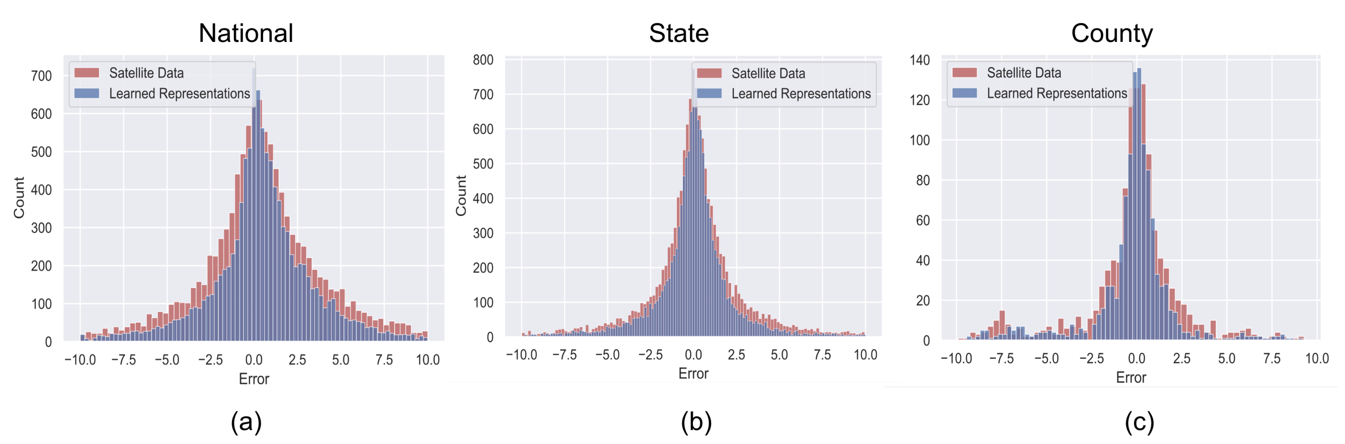
The error distributions of the satellite data and learned representations models are shown above in Figure 9. The learned representations consistently obtain lower errors than the satellite data on all three spatial scales. The magnitude of improvement in error is most visible in the national model, indicating the ability of the learned representations to help the model generalize to a large area.
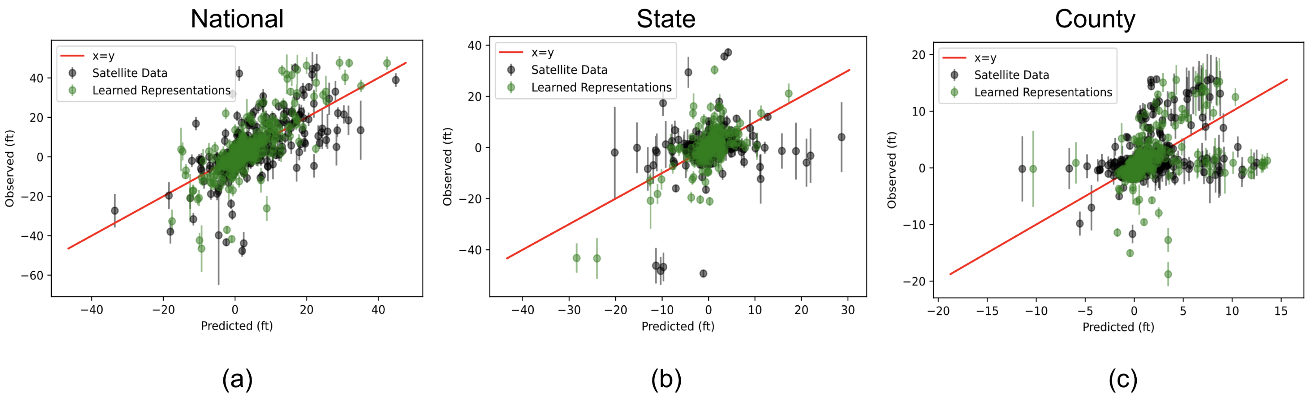
Scatterplots of model predictions vs. observed GWLA are shown at the three spatial scales above in Figure 10. Error bars were calculated with the algorithm developed by Wager et al. [28] in the forestci python package [29]. On the national and state scales, the satellite data models show a greater deviation from the observed, and their large error bars indicate a higher variability. Performance on the county model seems to be comparable for both the satellite data and learned representations model. This indicates that the learned representations provide the highest predictive power over large regions.
5. Discussion
This paper illustrates how a proof-of-concept unsupervised learning model can improve the accuracy of groundwater prediction models. This is the first time unsupervised learning techniques have been utilized for groundwater prediction.
Currently, the processed GRACE data are limited to one number for a 1 × 1 area. This coarse resolution limits the ability of GRACE to provide detailed groundwater signals and thus hinders the performance of groundwater prediction models.
In this model, GRACE data are contextualized by the surrounding GRACE and meteorological values in the “image”, which represents a 2 × 2 coordinate box. The learned representation depends on the entire context of the image, allowing it to elucidate fine-grained patterns in the data. Compared to the single GRACE number, this learned representation provides a much richer signal for prediction tasks. Thus, it effectively serves to downscale GRACE, helping overcome the main bottleneck in the literature [30]. While current downscaling methods tend to focus on a specific region or basin, the developed learned representations are applicable globally.
When fed as an input to groundwater prediction models, in lieu of raw satellite data, the learned representations significantly improve accuracy. This performance is achieved by training the Tile2Vec model on 20.6 million parameters. Training a larger model for more epochs will likely lead to larger improvements, as a common finding in the machine learning literature is that larger models lead to higher gains [31].
The Tile2Vec model was trained on global data to ensure the widespread usability of the resulting learned representations. However, to improve model performance even more, the addition of inputs such as soil data and Cropland Data Layer (CDL) could prove to be beneficial. With the potential to improve performance across virtually all groundwater prediction tasks, developing high-quality learned representations is a promising future direction for the field.
Through the use of novel machine learning techniques, this paper presents a way to improve the accuracy of groundwater predictions, aiding water management efforts across the globe.
6. Conclusions
With many regions of the world facing extreme groundwater drought, it is crucial that there is continuous information available to assess the degree of depletion. The status quo relies on dedicated monitoring wells, which are costly and difficult to maintain in low-resource settings. Efforts to remedy this include training machine learning models on satellite data, most notably GRACE. Cutting-edge machine learning techniques such as unsupervised representation learning have the potential to be of use in groundwater modeling, but their utilization has been severely limited. In this paper, unsupervised representation learning techniques were applied to the GRACE satellite, effectively “downscaling” the data. The resulting learned representations are able to reduce the RMSE by up to 19% and improve NSE by 8x at three different spatial scales, indicating their potential for widespread applications. These globally trained representations will allow for improved accuracy across a wide variety of machine learning-based groundwater prediction models, providing the information necessary to manage groundwater.
Funding
This research received no external funding.
Data Availability Statement
Pre-trained model weights, code, and datasets are available on Github at https://github.com/akhilapram/GRACE-Learned-Representations (accessed on 14 August 2022).
Conflicts of Interest
The author declares no conflict of interest.
Abbreviations
The following abbreviations are used in this manuscript:
| CLSM | Catchment Land Surface Model |
| GLDAS | Global Land Data Assimilation |
| GRACE | Gravity Recovery and Climate Experiment |
| GWLA | Groundwater Level Anomaly |
| MAR | Managed Aquifer Recharge |
| TWS | Terrestrial Water Storage |
| NSE | Nash–Sutcliffe Efficiency |
| RMSE | Root Mean Square Error |
| MAE | Mean Absolute Error |
References
- UN-Water. Groundwater overview: Making the invisible visible. Produced by International Groundwater Resources Assessment Centre, in cooperation with UNESCO-IHP, IAH, IWMI and with contributions of many UN-Water members and partners. 2018. Available online: https://www.unwater.org/publications/groundwater-overview-making-invisible-visible (accessed on 8 September 2022).
- Jasechko, S.; Perrone, D. Global groundwater wells at risk of running dry. Science 2021, 372, 418–421. [Google Scholar] [CrossRef] [PubMed]
- Salehi, M. Global water shortage and potable water safety; Today’s concern and tomorrow’s crisis. Environ. Int. 2022, 158, 106936. [Google Scholar] [CrossRef]
- Elshall, A.S.; Ye, M.; Wan, Y. Groundwater sustainability in a digital world. In Water and Climate Change; Elsevier: Amsterdam, The Netherlands, 2022; pp. 215–240. [Google Scholar]
- Priyan, K. Issues and challenges of groundwater and surface water management in semi-arid regions. Groundw. Resour. Dev. Plan. Semi-Arid Reg. 2021, 1–17. Available online: https://link.springer.com/chapter/10.1007/978-3-030-68124-1_1 (accessed on 6 September 2022).
- Choy, J. High Quality Groundwater Data Isn’t Always Easy or Cheap, But It Is Necessary. Standford Water West 2016. Available online: https://waterinthewest.stanford.edu/news-events/news-insights/high-quality-groundwater-data-isn%E2%80%99t-always-easy-or-cheap-it-necessary (accessed on 8 September 2022).
- Mogheir, Y.; De Lima, J.; Singh, V. Assessment of informativeness of groundwater monitoring in developing regions (Gaza Strip Case Study). Water Resour. Manag. 2005, 19, 737–757. [Google Scholar] [CrossRef]
- Dillon, P.; Stuyfzand, P.; Grischek, T.; Lluria, M.; Pyne, R.; Jain, R.; Bear, J.; Schwarz, J.; Wang, W.; Fernandez, E.; et al. Sixty years of global progress in managed aquifer recharge. Hydrogeol. J. 2019, 27, 1–30. [Google Scholar] [CrossRef]
- Condon, L.E.; Kollet, S.; Bierkens, M.F.; Fogg, G.E.; Maxwell, R.M.; Hill, M.C.; Fransen, H.J.H.; Verhoef, A.; Van Loon, A.F.; Sulis, M.; et al. Global groundwater modeling and monitoring: Opportunities and challenges. Water Resour. Res. 2021, 57, e2020WR029500. [Google Scholar] [CrossRef]
- Schumacher, M.; Forootan, E.; van Dijk, A.I.; Schmied, H.M.; Crosbie, R.S.; Kusche, J.; Döll, P. Improving drought simulations within the Murray-Darling Basin by combined calibration/assimilation of GRACE data into the WaterGAP Global Hydrology Model. Remote Sens. Environ. 2018, 204, 212–228. [Google Scholar] [CrossRef]
- Li, B.; Rodell, M.; Kumar, S.; Beaudoing, H.K.; Getirana, A.; Zaitchik, B.F.; de Goncalves, L.G.; Cossetin, C.; Bhanja, S.; Mukherjee, A.; et al. Global GRACE data assimilation for groundwater and drought monitoring: Advances and challenges. Water Resour. Res. 2019, 55, 7564–7586. [Google Scholar] [CrossRef]
- Mascarelli, A. Demand for Water Outstrips Supply. Nature 2012. Available online: https://www.nature.com/articles/nature.2012.11143.pdf?origin=ppub (accessed on 8 September 2022). [CrossRef]
- Ahmadi, A.; Olyaei, M.; Heydari, Z.; Emami, M.; Zeynolabedin, A.; Ghomlaghi, A.; Daccache, A.; Fogg, G.E.; Sadegh, M. Groundwater level modeling with machine learning: A systematic review and meta-analysis. Water 2022, 14, 949. [Google Scholar] [CrossRef]
- Ali, S.; Liu, D.; Fu, Q.; Cheema, M.J.M.; Pal, S.C.; Arshad, A.; Pham, Q.B.; Zhang, L. Constructing high-resolution groundwater drought at spatio-temporal scale using GRACE satellite data based on machine learning in the Indus Basin. J. Hydrol. 2022, 128295. [Google Scholar] [CrossRef]
- Ali, S.; Liu, D.; Fu, Q.; Cheema, M.J.M.; Pham, Q.B.; Rahaman, M.M.; Dang, T.D.; Anh, D.T. Improving the resolution of grace data for spatio-temporal groundwater storage assessment. Remote Sens. 2021, 13, 3513. [Google Scholar] [CrossRef]
- Gorugantula, S.S.; Kambhammettu, B.P. Sequential downscaling of GRACE products to map groundwater level changes in Krishna river basin. Hydrol. Sci. J. 2022. [Google Scholar] [CrossRef]
- Tao, H.; Hameed, M.M.; Marhoon, H.A.; Zounemat-Kermani, M.; Salim, H.; Sungwon, K.; Sulaiman, S.O.; Tan, M.L.; Sa’adi, Z.; Mehr, A.D.; et al. Groundwater level prediction using machine learning models: A comprehensive review. Neurocomputing 2022, 489, 271–308. [Google Scholar] [CrossRef]
- Mikolov, T.; Chen, K.; Corrado, G.; Dean, J. Efficient Estimation of Word Representations in Vector Space. arXiv 2013, arXiv:1301.3781. [Google Scholar] [CrossRef]
- Sivakumar, S.; Videla, L.S.; Kumar, T.R.; Nagaraj, J.; Itnal, S.; Haritha, D. Review on Word2Vec Word Embedding Neural Net. In Proceedings of the 2020 International Conference on Smart Electronics and Communication (ICOSEC), Trichy, India, 10–12 September 2020; pp. 282–290. [Google Scholar]
- Agastya, C.; Ghebremusse, S.; Anderson, I.; Vahabi, H.; Todeschini, A. Self-supervised Contrastive Learning for Irrigation Detection in Satellite Imagery. arXiv 2021, arXiv:2108.05484. [Google Scholar]
- Jean, N.; Wang, S.; Samar, A.; Azzari, G.; Lobell, D.; Ermon, S. Tile2vec: Unsupervised representation learning for spatially distributed data. Proc. AAAI Conf. Artif. Intell. 2019, 33, 3967–3974. [Google Scholar] [CrossRef]
- Rahaman, M.M.; Thakur, B.; Kalra, A.; Li, R.; Maheshwari, P. Estimating high-resolution groundwater storage from GRACE: A random forest approach. Environments 2019, 6, 63. [Google Scholar] [CrossRef]
- Walton, B. US Groundwater Losses Between 1900–2008: Enough To Fill Lake Erie Twice. Circ. Blue 2013. Available online: http://www.ashergrey.info/uploads/1/4/8/3/14835916/circleofblue.org-us_groundwater_losses_between_19002008_enough_to_fill_lake_erie_twice.pdf (accessed on 6 September 2022).
- Konikow, L.F. Groundwater Depletion in the United States (1900-2008); US Department of the Interior, US Geological Survey: Reston, VA, USA, 2013. [Google Scholar]
- Steward, D.R.; Bruss, P.J.; Yang, X.; Staggenborg, S.A.; Welch, S.M.; Apley, M.D. Tapping unsustainable groundwater stores for agricultural production in the High Plains Aquifer of Kansas, projections to 2110. Proc. Natl. Acad. Sci. USA 2013, 110, E3477–E3486. [Google Scholar] [CrossRef]
- Groundwater. Available online: https://www.dnr.state.mn.us/waters/groundwater_section/index.html (accessed on 8 September 2022).
- Miro, M.E.; Famiglietti, J.S. Downscaling GRACE remote sensing datasets to high-resolution groundwater storage change maps of California’s Central Valley. Remote Sens. 2018, 10, 143. [Google Scholar] [CrossRef]
- Wager, S.; Hastie, T.; Efron, B. Confidence intervals for random forests: The jackknife and the infinitesimal jackknife. J. Mach. Learn. Res. 2014, 15, 1625–1651. [Google Scholar] [PubMed]
- Polimis, K.; Rokem, A.; Hazelton, B. Confidence intervals for random forests in python. J. Open Source Softw. 2017, 2, 124. [Google Scholar] [CrossRef] [Green Version]
- Alley, W.M.; Konikow, L.F. Bringing GRACE down to earth. Groundwater 2015, 53, 826–829. [Google Scholar] [CrossRef]
- Jordan, M.I.; Mitchell, T.M. Machine learning: Trends, perspectives, and prospects. Science 2015, 349, 255–260. [Google Scholar] [CrossRef]
Figure 1.
Schematic diagram of Tile2Vec model framework.

Figure 2.
On the left, the model inaccurately characterizes the Euclidean distance between the learned representations of the anchor image and neighbor and distant images. Through unsupervised triplet loss, the model learns to minimize the distance between the representations of the anchor and neighbor images and maximize the distance between the representations of the anchor and distant images, as shown on the right.

Figure 3.
Satellite data “image” that is fed into the Tile2Vec model.

Figure 4.
Tile2Vec model training and validation loss curve.

Figure 5.
A satellite data “image” is fed into the trained unsupervised representation learning model. The resulting vector is fed into a random forest model that is trained on ground truth data (GWLA) to predict the groundwater level.
Figure 5.
A satellite data “image” is fed into the trained unsupervised representation learning model. The resulting vector is fed into a random forest model that is trained on ground truth data (GWLA) to predict the groundwater level.

Figure 6.
Distribution of ground-truth GWLA values for the national model.

Figure 7.
Distribution of ground-truth GWLA values for the state model.

Figure 8.
Distribution of ground-truth GWLA values for the county model.

Figure 9.
Histogram of error bars of the satellite data and learned representations Random Forest models: (a) national model, (b) state model, and (c) county model errors have been limited from —10 to 10 for better visibility.
Figure 9.
Histogram of error bars of the satellite data and learned representations Random Forest models: (a) national model, (b) state model, and (c) county model errors have been limited from —10 to 10 for better visibility.

Figure 10.
Scatterplots of satellite data and learned representations models performance with error bars: (a) national model, (b) state model, (c) county model. Random sample of 500 points for better visibility.
Figure 10.
Scatterplots of satellite data and learned representations models performance with error bars: (a) national model, (b) state model, (c) county model. Random sample of 500 points for better visibility.


Table 1.
Summary of input data used to estimate GWLA.
| Dataset | Source | Data Type | Units | Spatial Resolution | Temporal Resolution |
|---|---|---|---|---|---|
| GRACE TWS | JPL | Remote Sensing | cm | 1 × 1 | Monthly |
| Precipitation | GPM | Remote Sensing | mm | 0.1 × 0.1 | Monthly |
| Temperature | MERRA-2 | Remote Sensing | K | 0.5 × 0.625 | Monthly |
| Wind speed | GLDAS NOAH | Modeled | m/s | 0.25 × 0.25 | Monthly |
| Evapotranspiration | GLDAS NOAH | Modeled | kg/m/s | 0.25 × 0.25 | Monthly |
| Root zone soil moisture | GLDAS NOAH | Modeled | kg/m | 0.25 × 0.25 | Monthly |
| Baseflow groundwater runoff | GLDAS NOAH | Modeled | kg/m | 0.25 × 0.25 | Monthly |
| Plant canopy surface water | GLDAS NOAH | Modeled | kg/m | 0.25 × 0.25 | Monthly |
| Snow water equivalent | GLDAS NOAH | Modeled | kg/m | 0.25 × 0.25 | Monthly |
| Storm surface runoff | GLDAS NOAH | Modeled | kg/m | 0.25 × 0.25 | Monthly |
| Soil moisture | GLDAS NOAH | Modeled | kg/m | 0.25 × 0.25 | Monthly |
| Elevation | GLDAS Elevation | Modeled | m | 0.25 × 0.25 | Constant |
Table 2.
Results Summary.
| Metric | Learned Representations Model | Satellite Data Model | ||||
|---|---|---|---|---|---|---|
| United States | Minnesota | Stearns County | United States | Minnesota | Stearns County | |
| MAE (m) | 1.0241 | 0.6553 | 0.5303 | 1.2832 | 0.8013 | 0.6258 |
| Corr. Coeff. | 0.7830 | 0.4666 | 0.4144 | 0.6588 | 0.1667 | 0.2614 |
| NSE | 0.6131 | 0.2177 | 0.1718 | 0.4341 | 0.0277 | 0.0683 |
| Spearman Rho | 0.7324 | 0.5638 | 0.6075 | 0.6311 | 0.4701 | 0.4851 |
| RMSE (m) | 1.7678 | 1.3106 | 0.9753 | 2.1641 | 1.5240 | 1.036 |
Publisher’s Note: MDPI stays neutral with regard to jurisdictional claims in published maps and institutional affiliations. |
© 2022 by the author. Licensee MDPI, Basel, Switzerland. This article is an open access article distributed under the terms and conditions of the Creative Commons Attribution (CC BY) license (https://creativecommons.org/licenses/by/4.0/).
Share and Cite
MDPI and ACS Style
Ram, A.P. Unsupervised Representation Learning of GRACE Improves Groundwater Predictions. Water 2022, 14, 2947. https://doi.org/10.3390/w14192947
AMA Style
Ram AP. Unsupervised Representation Learning of GRACE Improves Groundwater Predictions. Water. 2022; 14(19):2947. https://doi.org/10.3390/w14192947
Chicago/Turabian StyleRam, Akhila Prabhakar. 2022. "Unsupervised Representation Learning of GRACE Improves Groundwater Predictions" Water 14, no. 19: 2947. https://doi.org/10.3390/w14192947
Note that from the first issue of 2016, this journal uses article numbers instead of page numbers. See further details here.