Article

Comparison of Microbial Profiling and Tracer Testing for the Characterization of Injector-Producer Interwell Connectivities

1
Department of Energy and Power Engineering, Tsinghua University, Beijing 100084, China
2
Department of Energy Resources Engineering, Stanford University, Stanford, CA 94305, USA
3
Department of Earth System Science, Stanford University, Stanford, CA 94305, USA
4
Robert Frederick Smith School of Chemical and Biomolecular Engineering, Cornell University, Ithaca, NY 14853, USA
5
Lawrence Berkeley National Laboratory, Berkeley, CA 94720, USA
6
School of Natural Sciences, Black Hills State University, Spearfish, SD 57799, USA
*
Authors to whom correspondence should be addressed.
Water 2022, 14(18), 2921; https://doi.org/10.3390/w14182921
Submission received: 27 August 2022 / Revised: 14 September 2022 / Accepted: 15 September 2022 / Published: 18 September 2022
(This article belongs to the Special Issue Hydrochemistry and Isotopes in Groundwater Investigations)

Abstract

:
Insufficient understanding of the microbial communities and associated microbial processes in geological reservoirs hinders the utilization of this rich data source for improved resource management. In this study, along with four interwell tracer tests at a 1478-m deep fractured crystalline-rock aquifer, we analyzed the microbial communities in the injected and produced water by high-throughput sequencing. The microbial community similarities across boreholes during an interwell flow scenario frequently encountered in reservoir development was explored. Despite the significant tracer recoveries (~30%) in all tracer tests and the cumulatively >100,000 L of exogenous water (carrying exogenous microbes) injected into the 10-m-scale reservoir, the overall structure of produced-fluid microbiome did not increasingly resemble that of the injectate. However, producers with better connectivity with the injector (based on tracer test results) did have more amplicon sequence variants (ASVs) that overlapped with those in the injectate. We identified possible drivers behind our observations and verified the practicality of repeated microbial sampling in the context of reservoir characterization and long-term monitoring. We highlight that injector-producer microbial profiling could provide insights on the relative connectivities across different producers with a given injector, and that the associated logistical needs may be comparable or even less than that of classic tracer tests.

1. Introduction

Microorganisms widely inhabit geological reservoirs and can affect or inform the exploitation of subsurface resources, such as groundwater [1,2,3], hydrocarbon [4,5,6,7,8] and geothermal energy [9,10], in various ways. Microbial community composition data of formation fluids, probed by modern high-throughput sequencing technology, is a rich data source that remains largely untapped in most subsurface reservoirs [1,2]. A thorough understanding of the microbial processes in geological reservoirs is the premise for utilizing microbial data for improved subsurface resource management. However, research on the deep biosphere is rare and usually hindered by limited sample accessibility [11]. Microbial data also pose challenges for the data assimilation of typical reservoir models because of both its high dimension (i.e., each datapoint consisting of thousands of microbial species) and the complex, coupled drivers behind the observed patterns that are still poorly understood.
Microbial processes in subsurface reservoirs can be classified into two major categories: metabolic [6,7,12,13,14,15,16] and hydrodynamic [17,18,19] (subcategories of deterministic process and stochastic process in microbial ecology [20,21,22], respectively). Metabolic processes refer to the change in microbial community composition after disturbance to reservoir environmental conditions (e.g., ionic concentrations, oxygen level, organic carbon availability, etc.) because different taxa have different physiologies, metabolic capabilities, and hence different levels of fitness to the changed environment [18,23]. For example, in aquifer systems, recharge events can significantly shift groundwater microbial communities by altering groundwater hydrochemical properties and stimulating the growth of opportunistic microbes [17,24,25]. In petroleum reservoirs, water injection is a common practice for enhanced oil recovery and/or hydraulic fracturing and is known to stimulate deleterious activities of sulfate-reducing bacteria that cause hydrogen sulfide production (i.e., souring) [6,7,14,15,16]. Hydrodynamic processes, on the other hand, refer to the passive dispersal capacity of microbial cells along with fluid flow because of their small body sizes. In deep, fractured aquifers where the energy-limited environment permits only extremely slow cell metabolism [26,27], natural or human-induced shifts in groundwater mixing could lead to variations in fluid-associated microbial community structure primarily by advective transport [18]. In shallow geological formations, hydrodynamic process can play important roles in microbial community dynamics as well [17,19].
In the context of subsurface resource extraction, the relative contribution of metabolic and hydrodynamic processes depends not only on the characteristics of the reservoir being developed, but also the specific type of reservoir operational scenarios. A reservoir can be water-based (e.g., groundwater and geothermal) or hydrocarbon-based (e.g., oil fields and shale). Reservoir operation can involve production of reservoir fluids under natural formation pressure or by pumping (i.e., primary production) [4], water injection to displace reservoir fluids out of a different well and/or hydraulically stimulate reservoir permeability (i.e., interwell displacement) [6,18], and injection/flowback into/from a single well (i.e., single well push-pull) [7]. A better understanding of the spatial and temporal patterns of microbial community structure under different scenarios provides not only grounds for utilizing microbial data for improved resource management, but also valuable insights for deep biosphere ecology research.
In this study, we analyzed the microbial community composition alongside four artificial tracer tests during a long-term flow test at a deep-subsurface aquifer with sparse permeable fractures. The repeated tracer tests were conducted in order to characterize the evolution of the interwell permeable fracture network over time [18,28,29,30]. Performed on or near the same date of microbial community analyses, the tracer test results also provided useful information for microbial data interpretation from a hydrodynamic perspective. The objective of this work is to compare the interwell tracer test data with the microbial community data of several injector-producer well pairs in a fractured reservoir. Patterns and correlations between the two types of data were identified, and the potential of injector-producer microbial profiling as a new tool for flowpath characterization was demonstrated. The significance and practicality of the two data sources for reservoir characterization were compared and discussed. Besides its practical value, this study also presents an example of the microbial community composition in a water-based reservoir, under an “interwell displacement” operational scenario (specifically, with a single injector and multiple producers). Our findings expand the current knowledge of microbial processes in deep geological reservoirs and may have implications for the microbial ecology under natural groundwater recharge events, such as by heavy rainfall or river intrusion.

2. Materials and Methods

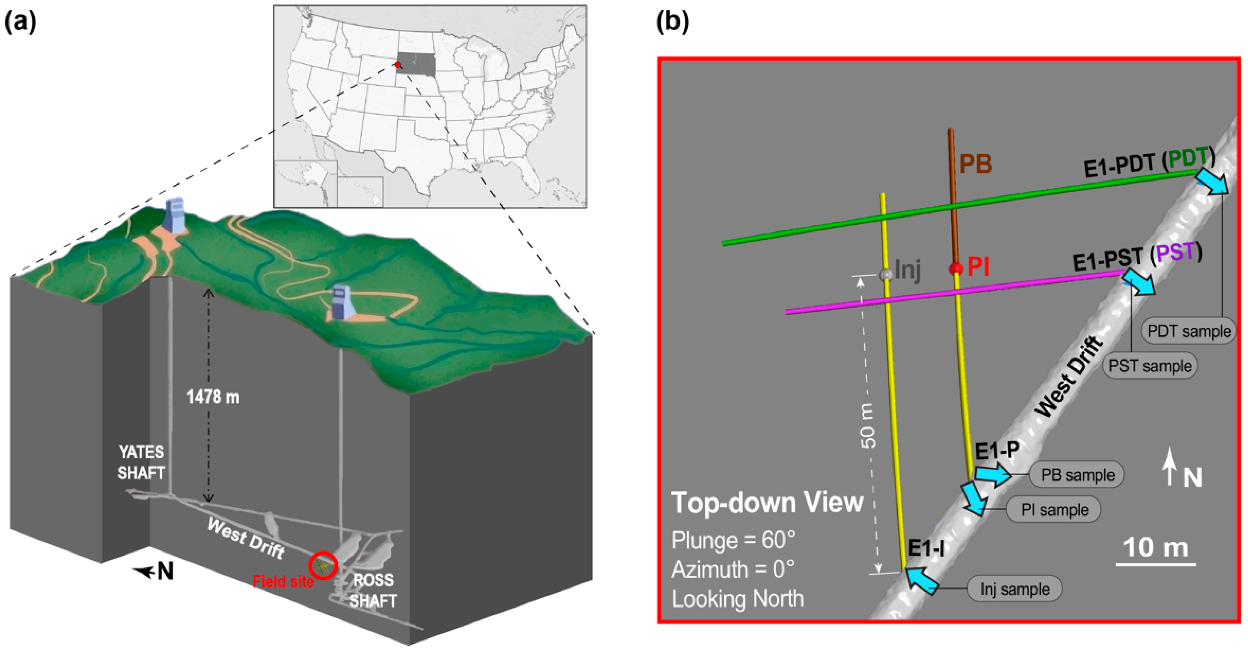
2.1. Enhanced Geothermal Systems (EGS) Collab Project Experiment 1: Field Site Description and Long-Term Flow Test

The field experiments were conducted at the EGS Collab Experiment 1 testbed at the Sanford Underground Research Facility (SURF) in Lead, South Dakota, USA. SURF is the former Homestake gold mine which became a dedicated science facility after mine closure in 2001 [1]. Located along the west mine drift 1478-m (4850-ft) below surface (Figure 1a), the mesoscale (10–100 m) testbed was within a naturally fractured aquifer with an active hydrologic system [31] and a dominant rock type of sericite-carbonate-quartz phyllite [32]. The testbed had a total of 8 60-m long boreholes drilled subhorizontally into the drift wall, 4 of which (E1-I, E1-P, E1-PDT, E1-PST) are relevant to this study hence are displayed in Figure 1b. The EGS Collab Experiment 1 included a 10-month (April 2019–February 2020) flow test between an injection borehole and several producing boreholes through a hydraulic-natural fracture network [18,33,34]. Throughout the flow test, mine industrial water (sourced from a shallow dolomitic limestone karst near SURF) was injected into the formation via a 1.8-m long straddle packer interval 50-m deep in borehole E1-I (henceforth referred to as Inj, as shown in Figure 1b), at a constant volumetric rate of 400 mL/min and a pressure up to 34.5 MPa. The constant injection pressurized the system and maintained outflow from 4 producing ports, E1-PDT, E1-PST, PI, and PB, at near atmospheric pressure. E1-PDT and E1-PST were 2 producing wells, whereas PI and PB refer to 2 segments along the same producing well E1-P and were hydraulically isolated by a set of straddle packers [18]. Throughout the rest of this paper, we will refer to the borehole segments with inflow or outflow as Inj, PDT, PST, PI, and PB (Figure 1b). Meanwhile, each borehole will be referred to as E1-I, E1-PDT, E1-PST, and E1-P. Note that E1-PDT and E1-PST are equivalent to PDT and PST, respectively, because the 2 wells were producing from their entire 60-m span (i.e., no straddle packers that isolate any segments in E1-PDT or E1-PST). Although PI and PB are 2 segments in the same well E1-P, they will henceforward be described as if they were 2 separate wells, for clarity. Total volumetric flow rate from the producing wells was initially ~70% of the injection rate, and gradually increased to ~98% near the end of the flow test [28,32].
Operational disturbance was minimized throughout the long-term flow test. Although disturbed briefly by unforeseen issues such as pump failures, the flow test continued largely uninterrupted throughout the 10-month time span (see details in [18]). The injected industrial water was initially at an ambient temperature of approximately 20 °C then chilled to 12 °C approximately 3 weeks after flow test initiation, although the outflow remained approximately 30 °C without significant temperature decrease (<1 °C) throughout the course of the flow test [18,32]. The reason for chilling the injectate was to investigate heat extraction in the context of EGS. For the purpose of this study, however, the chilling did not appear to have any direct influence on the comparison of microbial and tracer data and hence will not be further discussed.

2.2. Conservative Tracer Tests and Collection of Microbial Samples

Four conservative tracer tests [35,36] were conducted weeks to months apart during the 10-month flow test to characterize the flow pathways between Inj and each of the producing wells [28]. In each tracer test, a concentrated solution of carbon nanoparticle tracer (3–5 nm diameter, highly water soluble and inert) called “C-Dots” [37,38,39] was pushed into the main injection flow line by a dedicated ISCO pump, and its concentration was monitored in each producing well continuously for up to 2 days. Tracer samples were collected in 10-mL sampling tubes at a certain time interval (down to 10–20 min). The concentrations of C-Dot tracer were measured via fluorescence detection with excitation/emission wavelengths of 361/468 nm [28]. The tracer concentrations in the outflow were normalized by the concentration of the injected tracer pulse and plotted against cumulative volume produced to generate tracer breakthrough curves (BTCs) in each producing well.
On or near the date of each tracer campaign, microbial sampling was performed to analyze the microbial communities of the injected industrial water and the outflow from each producing well. On each date for microbial sampling, inflow into Inj as well as outflows from PDT, PST, PI, and PB were collected into 4-L acid-washed (5% hydrochloric acid) cubitainers until filled. The collected fluid samples were then passed through 0.22 µm Sterivex Duropore filters (EMD Millipore cat# SVGP01050) using sterile/acid-washed supplies to concentrate microbial cells onto the filters. The filters were frozen on site in dry ice and stored at −80 °C until analysis.
For a summary of tracer campaign dates and the nearest microbial sampling dates, see Table A1. Note that the microbial samples involved in this study belong to a 282-day microbial sampling campaign conducted roughly weekly from April 2019 to January 2020 and were partly described in our recent publication with a different focus [18]. Throughout the rest of this article, each tracer campaign will be referred to according to the date on which it was initiated (Table A1). Such naming fashion is consistent with other EGS Collab publications [28] and the metadata in our public data repository (see Data Availability Statement) for ease of comparison.

2.3. Genomic DNA Extraction, Library Preparation and 16S Ribosomal RNA (rRNA) Gene Amplicon Sequencing

DNA extraction from the filters and library preparation for 16S rRNA gene amplicon sequencing were performed according to the protocols detailed in [18]. Briefly, genomic DNA was extracted from each filter using the Qiagen AllPrep DNA/RNA Mini Kit (cat# 80204) following the manufacturer’s instructions with modifications to the cell disruption and DNA elution steps [18]. DNA yield was recorded for each extraction using a Qubit 3.0 fluorometer and the Qubit dsDNA High Sensitivity Assay Kit (Invitrogen cat# Q32851). The DNA yield was divided by the fluid sample volume that passed the entire filter accounting for the fraction of filter (usually half) extracted from, and the resulting concentration was divided by an approximate DNA mass per cell [40] to yield an approximate cell density (#cells/mL) in the fluid samples (described previously in [18]). Polymerase chain reaction (PCR) was performed on the extracted DNA using universal 16S primers 515F-Y/926R [41] which target the V4 and V5 hypervariable region of the 16S rRNA gene of both bacteria and archaea. A second-round PCR was conducted to add unique barcodes to the first-round PCR products (dual indexing). Blanks were included in every round of PCR with no amplification observed, confirming the absence of contaminants. The PCR products were cleaned up, pooled in equimolar concentrations, purified again, and sequenced on an Illumina MiSeq 2 × 250 bp paired-end sequencing platform at the UC Davis Genome Center.

2.4. High-Throughput Sequencing Data Processing

Primer sequences were trimmed from the raw sequencing reads using cutadapt [42]. The sequences were quality filtered by truncating reads beyond 220 bases so that bases with quality scores <30 were discarded. Sequences that did not exactly match proximal primers, had more than 2 expected errors, or contained ambiguous bases (Ns) were discarded as well. The high-resolution DADA2 method [43] was used for the inference of amplicon sequence variants (ASVs), removal of sequencing errors, merging forward and reverse sequencing reads allowing no mismatches in the overlap region, removal of chimeras, and generation of an ASV table. The ASVs were assigned taxonomy using the Silva v132 database implemented in DADA2 [44]. A phylogenetic tree of all ASVs was constructed using DECIPHER [45] and phangorn [46] in R to allow the calculation of phylogeny-aware distances between communities.

2.5. Diversity and Statistical Analyses

All diversity and statistical analyses on the sequencing data were performed in the R statistical software (version 4.0.2) [47]. Alpha diversity indices (Shannon and Inverse Simpson) were calculated using ‘estimate_richness’ function in phyloseq package. Note that the sequencing data was not rarefied in this study [17,48]. Rarefaction curves, however, were calculated to make sure the alpha diversity metrics had stabilized well before the minimum sequencing depth was reached (see Section 3.2). Beta diversity analysis was performed to evaluate the degree of differentiation in community compositions among all sample pairs using weighted Unifrac [49,50] as the distance metric. Weighted Unifrac distance takes into account not only the presence/absence of taxa and their relative abundance, but also their phylogenetic relatedness, giving distantly related taxa more weight than closely related taxa when calculating the distance. The weighted Unifrac distances among all sample pairs were first computed (function ‘Unifrac’ in phyloseq, using data at the ASV level) to generate a distance matrix, then hierarchical clustering was performed (“ward.D2” method in function ‘hclust’ in stats package) to visualize the distance matrix via a dendrogram. The number of overlapping ASVs among sampled wells over the period near each tracer campaign was calculated and visualized via Venn diagrams using function ‘venn’ in package eulerr.

3. Results

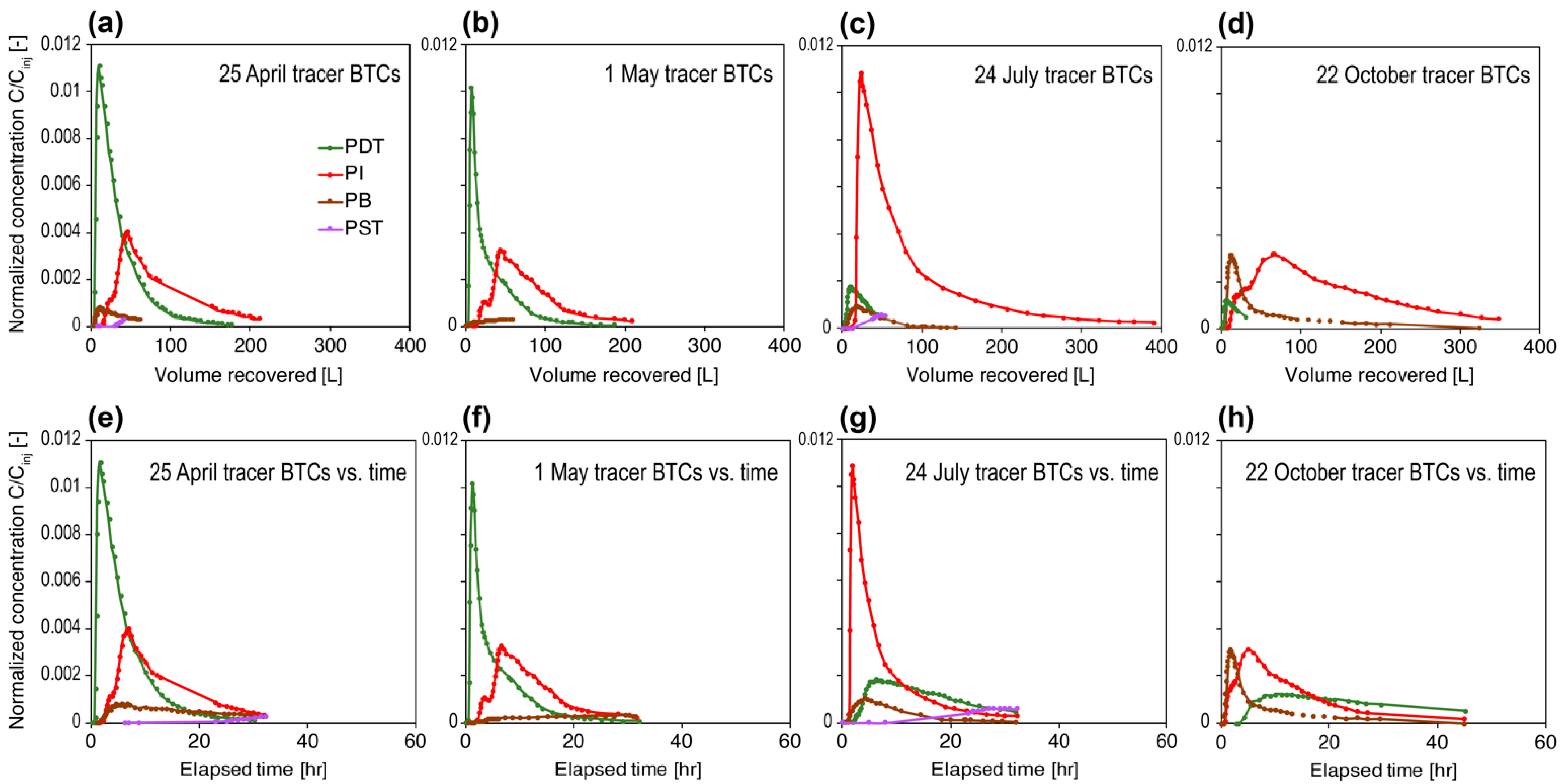
3.1. Long-Term Flow Test, Overall Geochemistry, and Tracer Data

The respective outflow rate in each producing well not only varied among wells, but also changed over time, indicative of a dynamically changing network of flowpaths [18,28,32]. The flow rate was highest in PI and PDT during the first two weeks of the flow test (~100 mL/min) while outflow from PB was <50 mL/min. Following this, however, PDT flow rate dropped to below 50 mL/min in June 2019 and remained below 50 mL/min thereafter, while flow rates in PI and PB increased to >200 mL/min and ~100 mL/min, respectively. The outflow from PST remained <50 mL/min throughout the long-term flow test. For the entire flow rate history, see [18] and [51].
Weekly geochemistry data (major cations and anions, pH, EC) for the produced and injected fluids during the long-term flow test was documented in [18]. Overall, fluids from all producing wells were dominated by sulfate (60–1250 mg/L), calcium (70–490 mg/L), magnesium (8–40 mg/L), and sodium (3–150 mg/L). In comparison, the ionic concentrations of the injectate were much lower and more stable over time, dominated by calcium (40–70 mg/L), magnesium (20–40 mg/L), and sulfate (3–6 mg/L). The pH of all fluids was within the range of 7 to 8 (pH strip measurements). The EC values were estimated based on geochemical data and ranged from 770–3800 μS/cm for PDT, 560–2360 μS/cm for PST, 410–2150 μS/cm for PI, 520–2150 μS/cm for PB, and 280–390 μS/cm for Inj [18].
Tracer breakthrough curves of each tracer campaign are shown in Figure 2. Normalized tracer concentrations are plotted against the cumulative volume recovered (since the start of each tracer test) to account for the differences in flow rate of each producing well [28] (Figure 2a–d). Tracer concentrations were also plotted against elapsed time as a reference (Figure 2e–h). Total tracer mass recoveries as well as the single-well recoveries were calculated according to [28] and summarized in Table 1. Total tracer recoveries were generally approximately 30% (±8%). Tracer first arrival in each producing well was generally on the order of an hour with peak arrival within 10 hr, which was rapid compared with full-scale geothermal reservoirs [28] but typical of mesoscale field tracer tests documented in the literature [52,53]. A prominent feature of the tracer test results is that the interwell connectivities for Inj-PDT, Inj-PI, and Inj-PB were different at a certain time point, and the relative connectivities across wells with the injector changed dramatically over time (Figure 2). Note that PST had a negligible amount of tracer detected in all tracer tests (ranging from 0 to 1.3% mass recoveries).

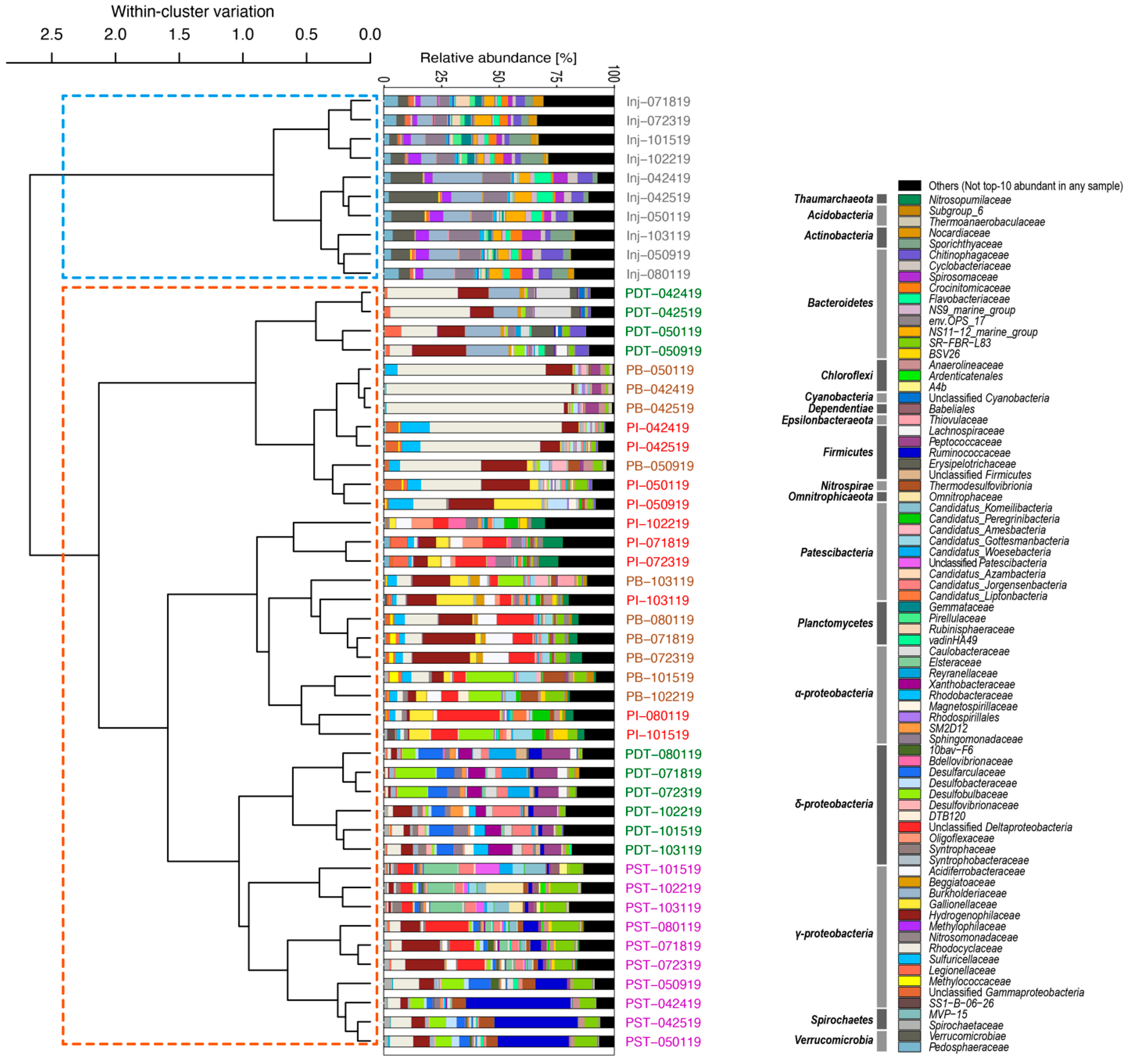
3.2. Microbial Community Compositions in the Produced Fluids Were Distinct from Those in the Injectate in All Four Tracer Campaigns

Among all the 50 microbial samples relevant to this study, there was an average of 32,216 reads per sample that passed the quality filter (~77.6% of the raw reads). All samples had over 10,000 reads that passed the quality filter. Over 95% of the samples had >10,000 inferred ASVs (minimum number of inferred ASVs was 7711). Rarefaction curves (Figure A1) confirm sufficient sequencing depth. Together with estimated cell concentrations of roughly 105 cells/mL in both the injected and the produced fluids (Figure A2), adequate sampling was confirmed for this study. A total of 4707 unique ASVs were identified. All ASVs were assigned taxonomy, grouped at the finest classification possible down to the family level, and the ASV table was visualized in stacked bar plots showing the relative abundance of each taxa in the whole microbial community of each fluid sample (Figure 3). The bar plots were arranged according to the order of the dendrogram leaves of the hierarchical clustering results. In other words, the bar plots were grouped according to their relative similarities (based on weighted Unifrac distance) for ease of interpretation.
As shown in Figure 3, despite the continuous injection of mine industrial water into the formation and the direct hydraulic connection between Inj and most producing wells as indicated by the rapid tracer breakthrough and substantial total tracer recovery (~30% ± 8%), the microbial communities in all produced fluids were distinct from those in the injectate. The major taxa in the injectate include the Spirosomaceae and Flavobacteriaceae belonging to the Bacteroidetes phylum, the alphaproteobacterial Sphingomonadaceae, the gammaproteobacterial Burkholderiaceae and Methylophilaceae, as well as members of the Verrucomicrobia phylum. In contrast, major taxa in the produced fluids include Nitrosopumilaceae belonging to Thaumarchaeota; Ignavibacteriales family SR-FBR-L83 (Bacteroidetes phylum); clostridial families of the Firmicutes phylum, such as Lachnospiraceae, Peptococcaceae, and Ruminococcaceae; Nitrospirae class Thermodesulfovibrionia; Omnitrophicaeota family Omnitrophaceae; multiple members of the Cand. Patescibacteria; gammaproteobacterial families Acidiferrobacteraceae, Gallionellaceae, Hydrogenophilaceae, Rhodocyclaceae, and Sulfuricellaceae; as well as deltaproteobacterial members, such as Desulfobulbaceae and Desulfarculaceae. This visually evident distinction between the injected and produced community structures is confirmed by the hierarchical clustering results, which identified two major clades (indicated by the two dashed squares overlaying the dendrogram in Figure 3) made up of solely injectate communities and solely produced fluids communities, respectively. Temporally, the injectate communities were quite stable, which is in stark contrast with the produced communities which changed dramatically with time. The driver behind the dynamic community structure in the produced fluids was likely the altered groundwater mixing caused by the changing fracture aperture and/or geometry, as discussed in detail in [18]. Alpha diversity analysis indicates that overall, communities in the produced fluids had lower diversity than those in the injectate (Figure 4).

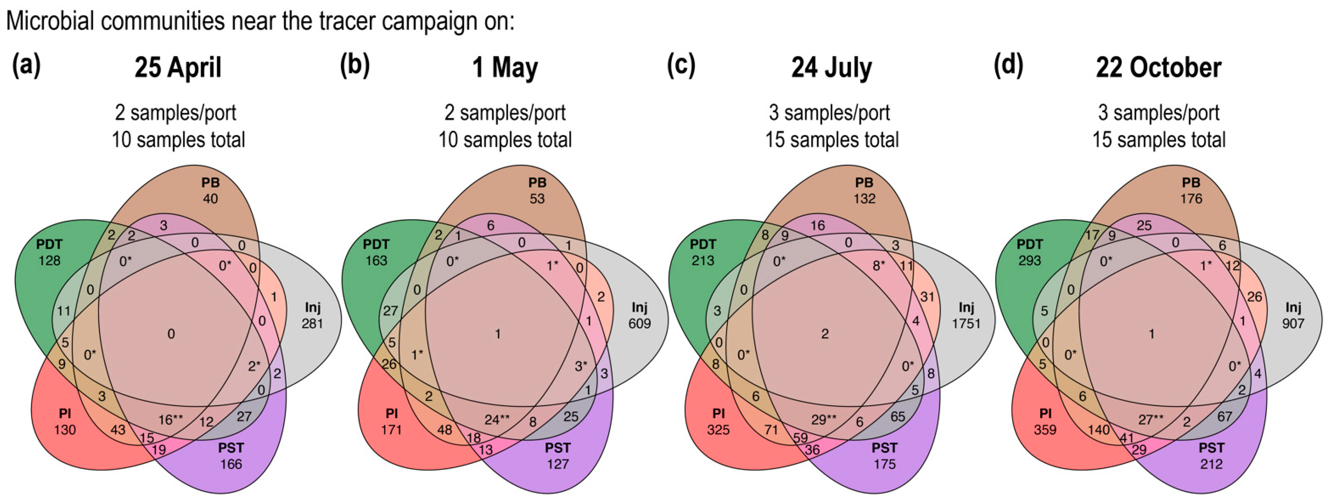
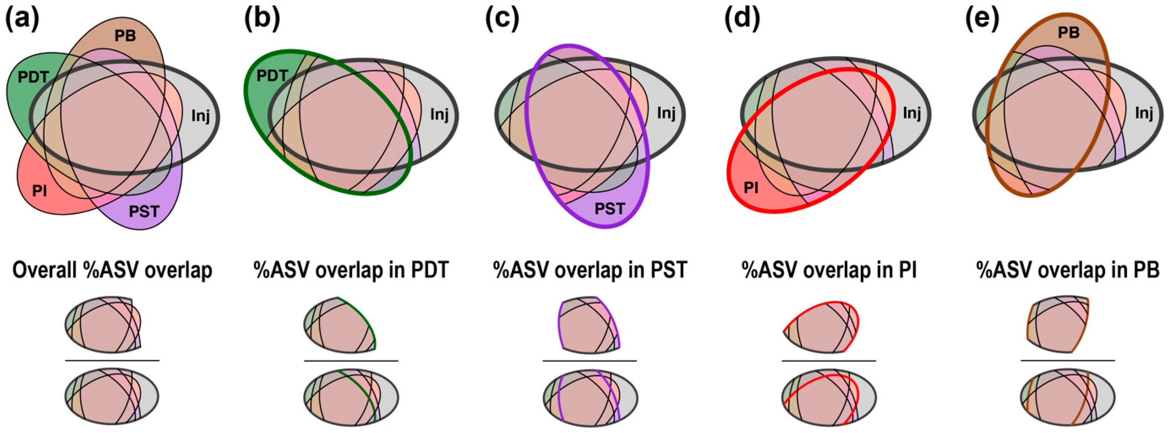
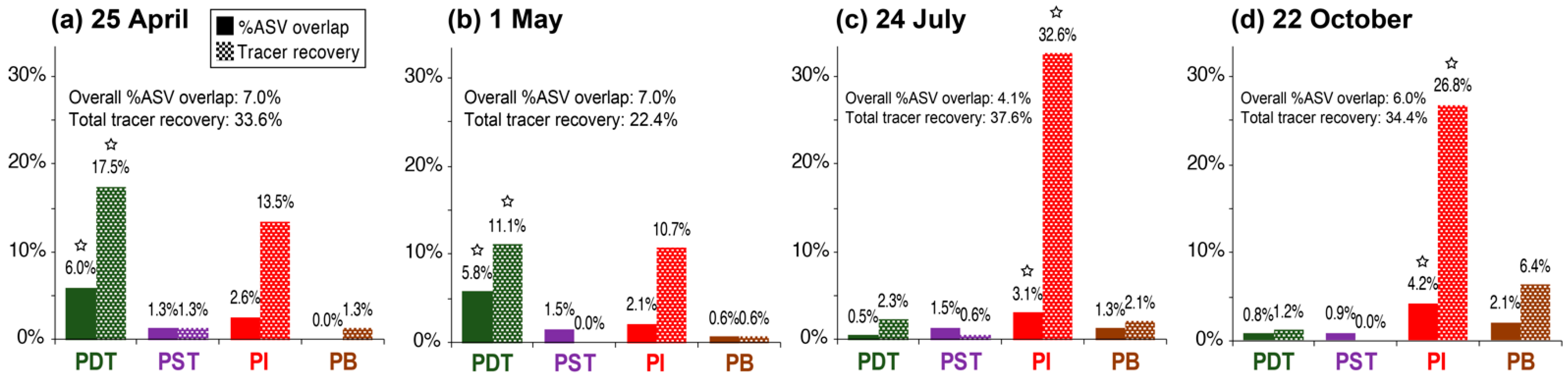
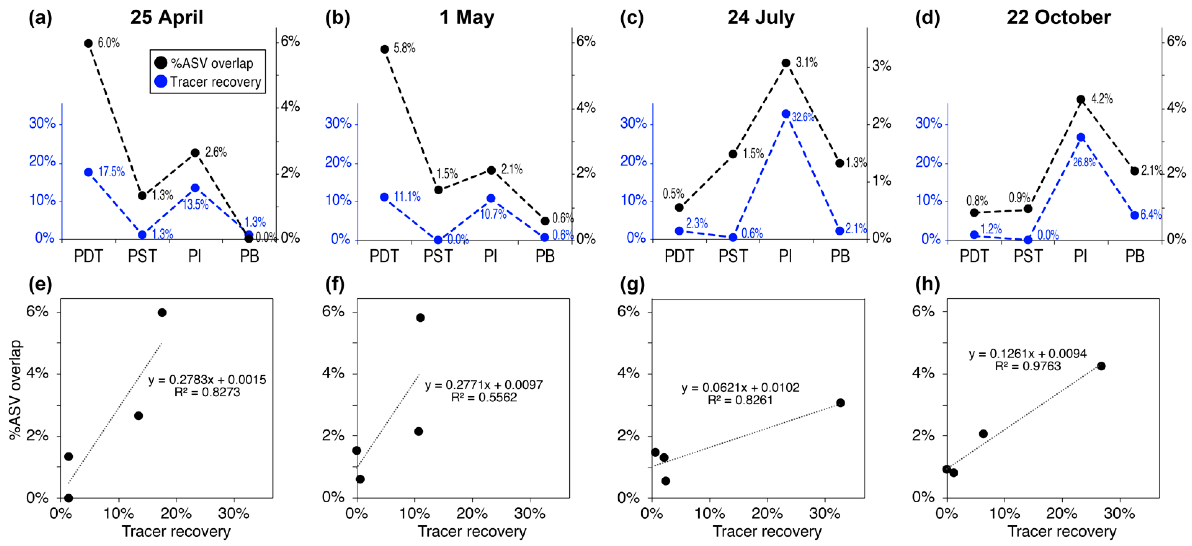
3.3. Trends in “%ASV Overlap” Metric Consistent with Trends in Tracer Recovery across Producing Wells

The microbial communities in the injectate and the produced fluids were further compared at the finest taxonomic resolution of the ASV level (i.e., differentiation between sequences that vary by down to one single nucleotide) by Venn diagram analysis. This method allows any common ASVs shared between the injectate and the produced fluids to be identified, even if the overlapping ASVs had such small relative abundances that they did not stand out in the relative abundance plot in Figure 3 and did not contribute much to the beta diversity analyses either. All sequences detected in each of the injection/production wells near the date of each tracer campaign (as defined in Table A1) were included in each Venn diagram analysis (Figure 5). Note that the Venn diagram considers only the presence/absence of unique ASVs, not their relative abundance.
Venn diagram analyses of the microbial communities in all four tracer campaigns showed a consistent lack of shared ASVs across all injection/producing wells, as indicated by the center values of merely two or fewer despite the hundreds to thousands of unique ASVs detected in each well in each tracer campaign. The number of shared ASVs among all four producing wells (indicated by two asterisks) is consistently larger than the number of shared ASVs among any other four wells (indicated by one asterisk). This further highlights the distinct injectate communities compared to those of the produced fluids.
To interpret the Venn diagram quantitatively, giving emphasis to the shared ASVs between injection-production well pairs, we define a “percentage of overlapping ASVs” metric (abbreviated as “%ASV overlap”). The %ASV overlap is calculated by dividing the total number of shared ASVs between a certain injection-production doublet (i.e., Inj-PDT, Inj-PST, Inj-PI, or Inj-PB) by the total number of unique ASVs in Inj, among the microbial samples near a certain tracer campaign (Figure 6). In other words, this metric represents the percentage of Inj ASVs that were also detected in each producing well near each tracer campaign. Overall %ASV overlap denotes the percentage of Inj ASVs that were also detected in any of the producing wells (Figure 6a). Using this method, each of the four Venn diagrams in Figure 5 gives four values of %ASV overlap along with an overall value, which reveals additional information on any similarities between communities from each producing well and those from the injectate. The calculated %ASV overlap metrics near each tracer campaign are displayed in Figure 7 alongside the single-well tracer recoveries.
The values of %ASV overlap between the injectate and each producing well remained small (only 0–6% as shown in Figure 7). However, the relative magnitude of %ASV overlap among producing wells is roughly consistent with their relative tracer recovery in each tracer campaign (Figure 8). For example, PDT had the largest C-Dot mass recovery of 17.5% and 11.1% in the 25 April and 1 May tracer campaigns, respectively. The largest %ASV overlap for microbial samples during the same time period were 6.0% and 5.8%, and were also from PDT (Figure 8a,b). In the 24 July and 22 October tracer tests, the largest C-Dot mass recoveries were from PI (32.6% and 26.8%, respectively). The largest %ASV overlap during that period were, interestingly, also from PI (3.1% and 4.2%, as shown in Figure 8c,d). Such consistency in relative %ASV overlap with tracer mass recovery is even true for the wells that had the second-largest tracer recoveries on 25 April (PI), 1 May (PI), and 22 October (PB), as shown in Figure 8. Cross-plotting %ASV overlap with tracer recovery values in each time period reveals a consistent positive correlation in all cases (Figure 8e–h).

4. Discussion

The focus of this study is to compare the conservative tracer data with microbial community data. We will, therefore, not go into much detail on the interpretation of tracer breakthrough curves themselves (covered in [28]), or the dynamics of the microbial communities (covered in [18]). The interwell tracer tests conducted at the EGS Collab testbed are typical examples of the “interwell displacement” operational scenario in a “water-based” reservoir, as classified earlier in this paper. The rapid, significant tracer breakthrough in at least one of the producing wells in all tracer campaigns indicates good hydraulic connection with the injection packer interval. Somewhat to our surprise, however, this months-long, continuous injection of exogenous water (cumulative volume on the order of 100,000 L as of late-October 2019) into the mesoscale fractured reservoir and the likely ~30% contribution of the injected water to the produced water (indicated by the tracer recovery) did not cause the microbial communities in the produced fluids to increasingly resemble those in the injectate. The %ASV overlap metric, on the other hand, showed trends roughly consistent with the relative recoveries in the tracer tests, although the absolute values of %ASV overlap remained much lower than the tracer recovery values. This suggests that a greater hydraulic connection between an injector-producer doublet did contribute to enhanced transport of injectate microorganisms toward the outlet to some extent. This enhancement, however, was very slight and did not have noticeable effect on the overall structure of microbial communities in the produced fluids.

4.1. Possible Reasons for the Limited Influence of Injectate Microbes on the Produced Microbial Community Profile

Groundwaters in deep geological reservoirs are populated with diverse native microorganisms that acquire energy through chemosynthesis without the need for sunlight [54,55]. An easy explanation for the distinction between the injected and produced communities is, therefore, that the produced fluids were mostly native groundwater displaced by the injected water. Native water originated from a distinct environment from the injected water and hence carried distinct microbial populations. The conservative tracer test results, however, suggested that the produced water did consist of a significant fraction of injected water in all four tracer tests (and hence likely throughout the April–October time span). In other words, the substantial volumetric contribution of injected water to the produced water did not result in the produced communities to resemble those of the injectate.

4.1.1. Retention of Injectate Microbes in Contrast with Mobility of Produced Microbes

One possible explanation for this phenomenon is cell retention. In fact, significant cell retainment in porous or fractured media after flow through (usually in the context of subsurface bioengineering or bioremediation research) has been reported frequently. Previous bacterial transport experiments through a ~30-m scale fractured, saturated crystalline bedrock have observed <4% recovery of injected bacterial culture despite >90% recovery of the conservative reference tracer [56]. Other researchers have observed >99% retention of injected bacteria in a sandy aquifer [57]. In laboratory-scale studies, cell retention in sand packs or sandstone cores was frequently reported as well [58,59,60], and in some cases, zero bacteria were detected in the outflow [61]. Plugging of pore throats by microbial cells can also occur [62].
At the EGS Collab Experiment 1 testbed, the major flow conduits included a natural fracture and a hydraulic fracture that intersected each other [18,33,34]. The rest of the formation was either tight rock matrix or sealed natural fractures with negligible permeability [18]. The natural fracture had a variable and overall large aperture up to several millimeters [1,33]. The hydraulic fracture, with which the injector packer interval intersected directly, had an estimated aperture below several hundred microns [34]. However, because fractures in the natural environment have spatially-varying apertures leading to tortuous flow pathways [63,64], microbial cells in the injectate may have been trapped at locations where the aperture was smaller than their cell size or where the fracture was partially closed. Alongside the size exclusion effect, microbial transport through fractures is additionally affected by the surface chemistry, morphology, and motility of each specific microbial strain, as well as chemical factors of the mineral surface [56,58]. Injectate microbes may have been attached to fracture surface sites to which the cell membranes have good affinity [56,58]. Motile microbes, in particular, may be especially prone to filtration because of their higher tendency to diffuse into the immobile water in small cracks/pores and get attached [56,65,66].
The potential tendency for introduced microbial cells to be retained in porous/fractured media, on the other hand, highlights the abundant indigenous microbes that did transport out of the aquifer. A notable category of the produced-fluid members is, interestingly, those with documented ultrasmall body size, for example, members of the phyla Patescibacteria (also known as the Candidate Phyla Radiation or CPR) and Omnitrophicaeota (also known as Omnitrophota, Omnitrophica or OP3) [67,68], both of which still lack culturable representatives, yet were found to be prevalent in oligotrophic groundwater environments worldwide in high abundance [25,67,68,69]. Among the 50 samples in this study, members of the Patescibacteria and Omnitrophicaeota phyla were prevalent and constituted up to 39.3% and 16.1% of the produced communities, respectively. In our recent study that encompassed the entire 282-day time-series microbial analysis of the EGS Collab Experiment-1 long-term flow test, an Omnitrophicaeota-affiliated ASV alone constituted 35.4% of the entire community in PST at one point [18]. In fact, ultrasmall cells have the evolutionary advantage that their increased surface-to-volume ratio optimizes the uptake of sparse nutrients in oligotrophic environments [69,70]. The lack of nutrients, in turn, further lead to reduction in cell size due to starvation [67,71]. Collectively, our observations along with past literature suggest that geological media may “select” for ultrasmall microorganisms by filtration. Future research on reservoir biotechnologies, especially those that involve injecting microbial cultures into the subsurface expecting microbes to travel extended distances, such as microbially induced carbonate precipitation (MICP) [60,61] and microbial enhanced oil recovery (MEOR) [72], could therefore consider focusing on native microorganisms with ready capabilities to migrate through geological media.

4.1.2. Survival Difficulty for Exogeneous Microbes

Besides physical retention, the injectate microbes that used to live in a shallow dolomitic aquifer may have difficulty surviving in deep groundwater due to unfitness to survive in the deep environment (e.g., high salinity, limited oxygen and nutrients, etc.) and competition with indigenous populations [73]. In fact, a number of field studies have observed the unlikely persistence of allochthonous microbes in groundwater environments [74,75,76]. The mean residence time for the C-Dots tracer in this work was several hours (Figure 2e–h), which might be too short for cell survival issues to matter. However, the residence time for the injected microbes can be longer than the inert tracer due to attachment to mineral surfaces or diffusion into smaller cracks [56,58,66]. Furthermore, the continuous input of injectate microbes (i.e., a “step input” as opposed to the “pulse input” of tracer) justifies considering the residence time of injected microbes (especially those potentially retained and accumulated in the aquifer) to be on the order of months. It is therefore possible that some injectate microbes gradually died and ended up as necromass for the survivors, and that their DNA eventually degraded and hence was not detectable in the effluent.

4.1.3. Undistinguishable Signal

In our field experiment, conducting microbial sampling is similar to performing tracer testing, in the sense that they both involved sampling the outflow to measure suspended/dissolved substances therein. However, it is important to recognize that the two processes are fundamentally different (see summary in Table 2):
  • In each tracer test, a chemical substance known to transport conservatively in fractured rocks [37] and with minimal/no background concentration was injected at a concentration much higher than its detection limit to allow sufficient room for dilution when flowed through the reservoir: typical strategies for tracer test designs. Tracer detection in the effluent is specific to the injected compound.
  • In contrast, on each microbial sampling date, the injectate water and fluids from each of the producing wells were simply collected into 4-L cubitainers until filled. The injectate contained hundreds to thousands of microbial species that were heavily diluted individually. It was not very likely that the injected exogenous microbes could transport conservatively (see Section 4.1.1). For any injectate microbes that managed to arrive at the producing wells, their DNA would be buried in the DNA of indigenous microbes when all ASVs were sequenced together.
Taken together, the observed distinction between injectate and produced communities, or in other words, the failure of injectate communities to prevail in the produced fluids, would seem fairly reasonable.

4.2. Percentage ASV Overlap as a New Indicator for Relative Interwell Connectivity

Despite the limited influence of injectate communities on the overall structure of produced fluid communities, there turned out to be subtle but informative trends in %ASV overlap between Inj and each producing well, as revealed by the Venn diagram analyses. The absolute values of %ASV overlap between each well pair were generally small (0–6%). However, the relative values of %ASV overlap among the four injection-production well pairs (i.e., Inj-PDT, Inj-PST, Inj-PI, and Inj-PB) near each tracer campaign had trends consistent with the trends in single-well tracer recoveries. We believe the driver behind such patterns is an increased probability that Inj ASVs will arrive at the better-connected producing well:
Consider the fraction of Inj ASVs that were also detected in each producing well (i.e., %ASV overlap) to comprise of two components: (1) ASVs that naturally existed in both this producing well and the injectate, and (2) ASVs in Inj that managed to migrate and arrive at this producing well. The possibility that component one (i.e., ubiquitous species) existed cannot be excluded. Since ubiquitous species, if present, are likely to be everywhere, here we assume it does not vary much across producing wells. Therefore, the trends in %ASV overlap would reflect trends in the probability for Inj ASVs to arrive at each producing well, and therefore could reflect the relative connectivities between the injection well and each of the producing wells.
Based on consistent observations across the four tracer campaigns described in this study, we propose the use of %ASV overlap metric as a new indicator for evaluating relative connectivities among different producers with a given injector. Keep in mind that the %ASV overlap metric should always be interpreted across producing wells (trends), rather than focusing on individual values (magnitudes). The magnitudes of the values are heavily influenced by the total number of unique ASVs in the injectate at the time of sampling, which is the denominator of the equation to calculate the %ASV overlap metric (as defined in Figure 6). Consequently, unlike classic tracer tests that can be informative for both single-producer and multi-producer field settings, %ASV overlap metric may only be informative when multiple producers are involved (i.e., when relative connectivity is of interest). Another factor to consider is the sequencing workflow. In this study, all samples were handled using the same sample/data processing protocols, including 16S primers, sequencing platform, raw data processing parameters, and so on. When the workflow varies among sequencing batches, care needs to be taken for such fine-resolution ASV-level comparisons to account for possible batch effects [2,11]. The %ASV overlap metric is based on the presence/absence of unique ASVs and does not consider abundance. Abundance data is subjected to a number of uncertainties, including variations of cell densities and sequencing depth, which is beyond the scope of this study. However, it might be a direction that deserves future research to further increase the informativeness of this novel data source.
Practically, microbial sampling to obtain %ASV overlap involves different sampling design and logistical needs compared with classic tracer testing, as summarized in Table 3. Based on our experience, although performing microbial sampling requires field personnel to be trained in aseptic sample handling and requires samples to be kept frozen/cold, once protocols were established, the microbial sampling was easily repeated in the long term. We were able to repeat the microbial sampling roughly weekly throughout the 10-month flow test (>30 sampling campaigns total, outlined in [18]), and one person performed the sampling from all five wells each time. In contrast, because tracer tests involved the delineation of a tracer breakthrough curve for every producing well and that each breakthrough curve typically consisted of 30–50 datapoints, a team of 3–4 people was usually needed in each tracer campaign to prepare and calibrate the tracer solution, to sample at high frequency, and to keep samples organized for on-site analysis or transportation to the laboratory. The sampling strategy may require real-time adjustment based on on-site measured tracer concentrations to optimize the capture of tracer plume at the producing wells [28]. Consequently, at least one person with tracer expertise and experience needs to be onsite to lead the team and make necessary decisions to ensure the success of the experiment. We suggest that both classic tracer tests and injector-producer microbial sampling have their advantages and drawbacks (Table 3). Future studies and field applications should select which method to adopt based on specific objectives and available resources.

4.3. Comparison with Similar Geological Systems

In recent years, high-throughput sequencing has been widely used to profile microbial communities in aquatic environments, including inland surface water [77,78], groundwater [1,12,17,18,79,80], and marine systems [81,82]. This information contributes to a better understanding of global biogeochemical cycles [11] as well as how animals/humans interact with the environment [9,83]. Practically, microbial community data can also be helpful in the management of engineered systems [1,6,8,18,77].
Groundwater reservoirs, in particular, are characterized by substantial spatial heterogeneity in terms of minerology, geochemistry, permeability, flow velocity, and so on [17,84,85,86]. Deep aquifers are additionally characterized by stable environmental conditions and hence stable structure of indigenous microbial communities [87] due to lack of impact from surface hydrological events [88]. In this work, we consider the injection of industrial water into the deep aquifer to be somewhat analogous to surface recharge events into shallow aquifers as described in previous studies [19,25]. These shallow aquifer studies observed community succession corresponding to periodic groundwater recharge but usually lacked microbial data of the recharge water. Therefore, the direct comparison between injected and produced microbiome achieved in this study can provide new insights into the mechanism behind previously reported patterns as well as the fate of allochthonous microbes in groundwater systems. However, keep in mind that our field setting is still markedly different from a shallow aquifer because of the much lower permeability of the geological media and the lack of diel/seasonal surface effects.
In the context of engineered geological systems, our field setting is typical of commercial geothermal reservoirs with reinjection, whereby wastewater is injected into the reservoir for disposal, pressure maintenance, and ultimately sustainable heat extraction [89]. However, to our knowledge, few studies have profiled the injector/producer microbial communities in such settings. In petroleum reservoirs, interwell displacement (i.e., “waterflooding”) is a common practice to displace residual oil and enhance productivity and has been extensively studied with respect to microbial diversity and metabolism [5,6,90]. However, hydrocarbon reservoirs are fundamentally different from groundwater reservoirs as microbial habitats because of the prevalence of organic carbon and the likely anthropogenic introduction of chemical additives [6,7,16]. The potential use of injector-producer microbial profiling for characterizing interwell connectivities in petroleum reservoirs, therefore, is an area that deserves further research.

5. Conclusions and Future Work

In summary, we found that on a one-year timescale, the continuous injection of exogeneous microbial communities into the deep-underground fractured aquifer did not cause the overall structure of produced-fluid microbiome to increasingly resemble that of the injectate, despite the tracer results which suggested significant contribution of the injected water to the produced water. However, the %ASV overlap metric proposed in this study was able to capture the subtle, increased similarities among highly connected wells in terms of shared ASVs, revealing trends in relative connectivities between injector-producer doublets consistent with conservative tracer test results. Given the unique logistical advantages of microbial analyses for standardized, repeated implementation, we further suggest that the combined microbial profiling of injected and produced fluids followed by %ASV overlap analyses may be a promising new tool for long-term reservoir monitoring. Future work is needed to compare the microbial communities in injected and produced water in other geological settings. Low-to-moderate temperature geothermal reservoirs with reinjection programs are especially interesting ecosystems to be further explored. The %ASV overlap metric can be further evaluated in future studies in groundwater, geothermal, and petroleum reservoirs, or readily applied as a novel means to monitor injector-producer interwell connectivities for subsurface engineering or scientific research purposes.

Author Contributions

Conceptualization, Y.Z., A.E.D. and R.N.H.; methodology, Y.Z., A.E.D. and R.N.H.; formal analysis, Y.Z.; investigation, Y.Z., A.J.H., J.C.P. and O.G.; resources, A.E.D. and R.N.H.; data curation, Y.Z.; writing—original draft preparation, Y.Z.; writing—review and editing, A.E.D., A.J.H., J.C.P., O.G. and R.N.H.; visualization, Y.Z.; supervision, A.E.D. and R.N.H.; project administration, Y.Z., A.E.D. and R.N.H.; funding acquisition, Y.Z., A.E.D. and R.N.H. All authors have read and agreed to the published version of the manuscript.

Funding

This material was based upon work supported by the US Department of Energy, Office of Energy Efficiency and Renewable Energy, Office of Technology Development, Geothermal Technologies Office, under Award Number DE-AC02-05CH11231 and subcontract agreement 7348695 with Stanford University. Additional support was from TomKat Center for Sustainable Energy at Stanford University under Award DekasHorne2018. Support from the Shuimu Tsinghua Scholar Program at Tsinghua University (No. 2020SM014) and the Chinese International Postdoctoral Exchange Fellowship Program (Talent-Introduction Program) No. YJ20200102 for the first author during the manuscript writing phase is acknowledged.

Data Availability Statement

Sequencing data was deposited in the European Nucleotide Archive at the European Bioinformatics Institute under accession no. PRJEB44691. Raw tracer data is publicly available through the US Department of Energy’s Geothermal Data Repository at: [91].

Acknowledgments

The research supporting this work took place in part at the SURF in Lead, SD. The assistance of the SURF and its personnel in providing physical access and general logistical and technical support is acknowledged. This work is one of the contributions of the Enhanced Geothermal Systems (EGS) Collab Team. We would like to specifically thank Timothy Kneafsey, Paul Schwering, Megan Smith, Parker Sprinkle, and the entire EGS Collab team for making the sampling possible. We also thank Cynthia Anderson and Dave Berggmann from Black Hills State University for providing additional resources near the site.

Conflicts of Interest

The authors declare no conflict of interest.

Appendix A. Dates of Tracer Test and Microbial Sampling Campaigns

Table A1. Summary of tracer campaign dates and each tracer campaign’s closest microbial sampling dates. Note that on each microbial sampling date, one microbial sample was obtained from each of the five wells (Inj, PDT, PST, PI, and PB). Ten microbial sampling dates with five samples total per date leads to a total of 50 microbial samples relevant to this study.
Tracer Campaign DateMicrobial Samples Near the Date of This Campaign
25 April24 April
25 April
1 May1 May
9 May
24 July18 July
23 July
1 August
22 October15 October
22 October
31 October

Appendix B. Quality Assurance of Sequencing Data

Figure A1. Rarefaction curves for the microbial sample set based on Shannon and Inverse Simpson diversity indices. Shannon and Inverse Simpson indices stabilized well before the minimum sequencing depth across all samples (7711 ASVs) was reached.
Water 14 02921 g0a1
Figure A2. Cell density from each well estimated from the yield of DNA extractions, displayed as box (and whisker) plots. The thick black horizontal line within each box denotes the median of the distribution of the 10 samples from each well. The bounds of the y-axis were selected based on previously observed cell concentration values in continental subsurface fluids [11].
Water 14 02921 g0a2

References

  1. Zhang, Y.; Dekas, A.E.; Hawkins, A.J.; Parada, A.E.; Gorbatenko, O.; Li, K.; Horne, R.N. Microbial Community Composition in Deep—Subsurface Reservoir Fluids Reveals Natural Interwell Connectivity. Water Resour. Res. 2020, 56, e2019WR025916. [Google Scholar] [CrossRef]
  2. Merino, N.; Jackson, T.R.; Campbell, J.H.; Kersting, A.B.; Sackett, J.; Fisher, J.C.; Bruckner, J.C.; Zavarin, M.; Hamilton-Brehm, S.D.; Moser, D.P. Subsurface microbial communities as a tool for characterizing regional-scale groundwater flow. Sci. Total. Environ. 2022, 842, 156768. [Google Scholar] [CrossRef] [PubMed]
  3. Overholt, W.A.; Trumbore, S.; Xu, X.; Bornemann, T.L.V.; Probst, A.J.; Krüger, M.; Herrmann, M.; Thamdrup, B.; Bristow, L.A.; Taubert, M.; et al. Carbon fixation rates in groundwater similar to those in oligotrophic marine systems. Nat. Geosci. 2022, 15, 561–567. [Google Scholar] [CrossRef]
  4. Kobayashi, H.; Endo, K.; Sakata, S.; Mayumi, D.; Kawaguchi, H.; Ikarashi, M.; Miyagawa, Y.; Maeda, H.; Sato, K. Phylogenetic diversity of microbial communities associated with the crude-oil, large-insoluble-particle and formation-water components of the reservoir fluid from a non-flooded high-temperature petroleum reservoir. J. Biosci. Bioeng. 2012, 113, 204–210. [Google Scholar] [CrossRef] [PubMed]
  5. Orphan, V.J.; Taylor, L.T.; Hafenbradl, D.; Delong, E.F. Culture-dependent and culture-independent characterization of microbial assemblages associated with high-temperature petroleum reservoirs. Appl. Environ. Microbiol. 2000, 66, 700–711. [Google Scholar] [CrossRef]
  6. Vigneron, A.; Alsop, E.B.; Lomans, B.P.; Kyrpides, N.C.; Head, I.M.; Tsesmetzis, N. Succession in the petroleum reservoir microbiome through an oil field production lifecycle. ISME J. 2017, 11, 2141–2154. [Google Scholar] [CrossRef] [PubMed]
  7. Cluff, M.A.; Hartsock, A.; MacRae, J.D.; Carter, K.; Mouser, P.J. Temporal changes in microbial ecology and geochemistry in produced water from hydraulically fractured Marcellus shale gas wells. Environ. Sci. Technol. 2014, 48, 6508–6517. [Google Scholar] [CrossRef]
  8. Hull, N.M.; Rosenblum, J.S.; Robertson, C.E.; Harris, J.K.; Linden, K.G. Succession of toxicity and microbiota in hydraulic fracturing flowback and produced water in the Denver-Julesburg Basin. Sci. Total. Environ. 2018, 644, 183–192. [Google Scholar] [CrossRef]
  9. Valeriani, F.; Gianfranceschi, G.; Spica, V.R. The microbiota as a candidate biomarker for SPA pools and SPA thermal spring stability after seismic events. Environ. Int. 2020, 137, 105595. [Google Scholar] [CrossRef]
  10. Power, J.F.; Carere, C.R.; Lee, C.K.; Wakerley, G.L.J.; Evans, D.W.; Button, M.; White, D.; Climo, M.D.; Hinze, A.M.; Morgan, X.C.; et al. Microbial biogeography of 925 geothermal springs in New Zealand. Nat. Commun. 2018, 9, 2876. [Google Scholar] [CrossRef] [Green Version]
  11. Magnabosco, C.; Lin, L.H.; Dong, H.; Bomberg, M.; Ghiorse, W.; Stan-Lotter, H.; Pedersen, K.; Kieft, T.L.; van Heerden, E.; Onstott, T.C. The biomass and biodiversity of the continental subsurface. Nat. Geosci. 2018, 11, 707–717. [Google Scholar] [CrossRef]
  12. Ben Maamar, S.; Aquilina, L.; Quaiser, A.; Pauwels, H.; Michon-Coudouel, S.; Vergnaud-Ayraud, V.; Labasque, T.; Roques, C.; Abbott, B.W.; Dufresne, A. Groundwater Isolation Governs Chemistry and Microbial Community Structure along Hydrologic Flowpaths. Front. Microbiol. 2015, 6, 1457. [Google Scholar] [CrossRef] [PubMed]
  13. Bochet, O.; Bethencourt, L.; Dufresne, A.; Farasin, J.; Pédrot, M.; Labasque, T.; Chatton, E.; Lavenant, N.; Petton, C.; Abbott, B.W.; et al. Iron-oxidizer hotspots formed by intermittent oxic–anoxic fluid mixing in fractured rocks. Nat. Geosci. 2020, 13, 149–155. [Google Scholar] [CrossRef]
  14. Tsesmetzis, N.; Alsop, E.B.; Vigneron, A.; Marcelis, F.; Head, I.M.; Lomans, B.P. Microbial community analysis of three hydrocarbon reservoir cores provides valuable insights for the assessment of reservoir souring potential. Int. Biodeterior. Biodegrad. 2018, 126, 177–188. [Google Scholar] [CrossRef]
  15. Youssef, N.; Elshahed, M.S.; McInerney, M.J. Microbial processes in oil fields: Culprits, problems, and opportunities. Adv. Appl. Microbiol. 2009, 66, 141–251. [Google Scholar]
  16. Daly, R.A.; Borton, M.A.; Wilkins, M.J.; Hoyt, D.W.; Kountz, D.J.; Wolfe, R.A.; Welch, S.A.; Marcus, D.N.; Trexler, R.V.; MacRae, J.D.; et al. Microbial metabolisms in a 2.5-km-deep ecosystem created by hydraulic fracturing in shales. Nat. Microbiol. 2016, 2016, 16146. [Google Scholar] [CrossRef]
  17. Yan, L.; Herrmann, M.; Kampe, B.; Lehmann, R.; Totsche, K.U.; Kusel, K. Environmental selection shapes the formation of near-surface groundwater microbiomes. Water. Res. 2020, 170, 115341. [Google Scholar] [CrossRef]
  18. Zhang, Y.; Horne, R.N.; Hawkins, A.J.; Primo, J.C.; Gorbatenko, O.; Dekas, A.E. Geological activity shapes the microbiome in deep-subsurface aquifers by advection. Proc. Natl. Acad. Sci. USA 2022, 119, e2113985119. [Google Scholar] [CrossRef]
  19. Lin, X.; McKinley, J.; Resch, C.T.; Kaluzny, R.; Lauber, C.L.; Fredrickson, J.; Knight, R.; Konopka, A. Spatial and temporal dynamics of the microbial community in the Hanford unconfined aquifer. ISME J. 2012, 6, 1665–1676. [Google Scholar] [CrossRef]
  20. Stegen, J.C.; Lin, X.; Konopka, A.E.; Fredrickson, J.K. Stochastic and deterministic assembly processes in subsurface microbial communities. ISME J. 2012, 6, 1653–1664. [Google Scholar] [CrossRef]
  21. Stegen, J.C.; Lin, X.; Fredrickson, J.K.; Chen, X.; Kennedy, D.W.; Murray, C.J.; Rockhold, M.L.; Konopka, A. Quantifying community assembly processes and identifying features that impose them. ISME J. 2013, 7, 2069–2079. [Google Scholar] [CrossRef] [PubMed]
  22. Ning, D.; Deng, Y.; Tiedje, J.M.; Zhou, J. A general framework for quantitatively assessing ecological stochasticity. Proc. Natl. Acad. Sci. USA 2019, 116, 16892–16898. [Google Scholar] [CrossRef] [PubMed]
  23. Stegen, J.C.; Lin, X.; Fredrickson, J.K.; Konopka, A.E. Estimating and mapping ecological processes influencing microbial community assembly. Front. Microbiol. 2015, 6, 370. [Google Scholar] [CrossRef] [PubMed]
  24. Wu, M.; Wang, H.; Wang, W.; Song, Y.; Ma, L.; Lu, X.; Wang, N.; Liu, C. The impact of heavy rain event on groundwater microbial communities in Xikuangshan, Hunan Province, P.R. China. J. Hydrol. 2021, 595, 125674. [Google Scholar] [CrossRef]
  25. Yan, L.; Hermans, S.M.; Totsche, K.U.; Lehmann, R.; Herrmann, M.; Kusel, K. Groundwater bacterial communities evolve over time in response to recharge. Water Res. 2021, 201, 117290. [Google Scholar] [CrossRef] [PubMed]
  26. Jorgensen, B.B. Deep subseafloor microbial cells on physiological standby. Proc. Natl. Acad. Sci. USA 2011, 108, 18193–18194. [Google Scholar] [CrossRef]
  27. Bar-On, Y.M.; Phillips, R.; Milo, R. The biomass distribution on Earth. Proc. Natl. Acad. Sci. USA 2018, 115, 6506–6511. [Google Scholar] [CrossRef]
  28. Neupane, G.; Mattson, E.; Plummer, M.; Podgorney, R. Results of Multiple Tracer Injections into Fractures in the EGS Collab Testbed-1. In Proceedings of the 45th Workshop on Geothermal Reservoir Engineering, Stanford, CA, USA, 10–12 February 2020. [Google Scholar]
  29. Kneafsey, T.J.; Dobson, P.F.; Blankenship, D.; Schwering, P.C.; Morris, J.P.; Fu, P.; Wu, H.; White, M.D.; Knox, H.A.; Ajo-Franklin, J.B.; et al. Field Experiments and Model Validation: The EGS Collab Project. In Proceedings of the 55th U.S. Rock Mechanics/Geomechanics Symposium, Houston, TX, USA, 20–23 June 2021. [Google Scholar]
  30. Kneafsey, T.; Blankenship, D.; Dobson, P.F.; Morris, J.; Fu, P.; White, M.; Schwering, P.; Knox, H.; Guglielmi, Y.; Schoenball, M.; et al. The EGS collab project: Stimulating and simulating experiments in crystalline rock in an underground research site. In Proceedings of the Geothermal Resources Council Virtual Annual Meeting and Expo: Clean, Renewable and Always On, GRC 2020, Virtual, 19–23 October 2020. [Google Scholar]
  31. Murdoch, L.C.; Germanovich, L.N.; Wang, H.; Onstott, T.C.; Elsworth, D.; Stetler, L.; Boutt, D. Hydrogeology of the vicinity of Homestake mine, South Dakota, USA. Hydrogeol. J. 2011, 20, 27–43. [Google Scholar] [CrossRef]
  32. Kneafsey, T.J.; Blankenship, D.; Dobson, P.F.; Morris, J.P.; White, M.D.; Fu, P.; Schwering, P.C.; Ajo-Franklin, J.B.; Huang, L.; Schoenball, M.; et al. The EGS Collab Project—Learnings from Experiment 1. In Proceedings of the 45th Workshop on Geothermal Reservoir Engineering, Stanford, CA, USA, 10–12 February 2020. [Google Scholar]
  33. Fu, P.; Schoenball, M.; Ajo-Franklin, J.B.; Chai, C.; Maceira, M.; Morris, J.P.; Wu, H.; Knox, H.; Schwering, P.C.; White, M.D.; et al. Close Observation of Hydraulic Fracturing at EGS Collab Experiment 1: Fracture Trajectory, Microseismic Interpretations, and the Role of Natural Fractures. J. Geophys. Res. Solid Earth 2021, 126, e2020JB020840. [Google Scholar] [CrossRef]
  34. Wu, H.; Fu, P.; Morris, J.P.; Mattson, E.D.; Neupane, G.; Smith, M.M.; Hawkins, A.J.; Zhang, Y.; Kneafsey, T. Characterization of flow and transport in a fracture network at the EGS Collab field experiment through stochastic modeling of tracer recovery. J. Hydrol. 2021, 593, 125888. [Google Scholar] [CrossRef]
  35. Zhang, Y.; Hartung, M.B.; Hawkins, A.J.; Dekas, A.E.; Li, K.; Horne, R.N. DNA Tracer Transport Through Porous Media—The Effect of DNA Length and Adsorption. Water Resour. Res. 2021, 57, 2020WR028382. [Google Scholar] [CrossRef]
  36. Zhang, Y.; Manley, T.S.; Li, K.; Home, R.N. DNA-Encapsulated silica nanoparticle tracers for fracture characterization. In Proceedings of the 39th Geothermal Resources Council Annual Meeting—Geothermal: Always On, GRC 2015, Reno, NV, USA, 20–23 September 2015. [Google Scholar]
  37. Hawkins, A.J.; Fox, D.B.; Becker, M.W.; Tester, J.W. Measurement and simulation of heat exchange in fractured bedrock using inert and thermally degrading tracers. Water Resour. Res. 2017, 53, 1210–1230. [Google Scholar] [CrossRef]
  38. Krysmann, M.J.; Kelarakis, A.; Dallas, P.; Giannelis, E.P. Formation mechanism of carbogenic nanoparticles with dual photoluminescence emission. J. Am. Chem. Soc. 2012, 134, 747–750. [Google Scholar] [CrossRef] [PubMed]
  39. Li, Y.V.; Cathles, L.M.; Archer, L.A. Nanoparticle tracers in calcium carbonate porous media. J. Nanopart. Res. 2014, 16, 2541. [Google Scholar] [CrossRef]
  40. Button, D.K.; Robertson, B.R. Determination of DNA content of aquatic bacteria by flow cytometry. Appl. Environ. Microbiol. 2001, 67, 1636–1645. [Google Scholar] [CrossRef]
  41. Parada, A.E.; Needham, D.M.; Fuhrman, J.A. Every base matters: Assessing small subunit rRNA primers for marine microbiomes with mock communities, time series and global field samples. Environ. Microbiol. 2016, 18, 1403–1414. [Google Scholar] [CrossRef]
  42. Martin, M. Cutadapt removes adapter sequences from high-throughput sequencing reads. EMBnet J. 2011, 17, 10–12. [Google Scholar] [CrossRef]
  43. Callahan, B.J.; PMcMurdie, J.; Holmes, S.P. Exact sequence variants should replace operational taxonomic units in marker-gene data analysis. ISME J. 2017, 11, 2639–2643. [Google Scholar] [CrossRef]
  44. Callahan, B.J. Silva Taxonomic Training Data Formatted for DADA2 (Silva Version 132) [Data Set]; Zenodo: Genève, Switzerland, 2018. [Google Scholar]
  45. Wright, E.S. Using DECIPHER v2.0 to Analyze Big Biological Sequence Data in R. R J. 2016, 8, 352. [Google Scholar] [CrossRef]
  46. Schliep, K.P. Phangorn: Phylogenetic analysis in R. Bioinformatics 2011, 27, 592–593. [Google Scholar] [CrossRef]
  47. R Core Team. R: A Language and Environment for statistical Computing; R Foundation for Statistical Computing: Vienna, Austria, 2020. [Google Scholar]
  48. McMurdie, P.J.; Holmes, S. Waste not, want not: Why rarefying microbiome data is inadmissible. PLoS Comput. Biol. 2014, 10, e1003531. [Google Scholar] [CrossRef] [PubMed] [Green Version]
  49. Lozupone, C.; Knight, R. UniFrac: A new phylogenetic method for comparing microbial communities. Appl. Environ. Microbiol. 2005, 71, 8228–8235. [Google Scholar] [CrossRef] [PubMed]
  50. Lozupone, C.A.; Hamady, M.; Kelley, S.T.; Knight, R. Quantitative and qualitative beta diversity measures lead to different insights into factors that structure microbial communities. Appl. Environ. Microbiol. 2007, 73, 1576–1585. [Google Scholar] [CrossRef] [PubMed]
  51. Knox, H.; Linneman, D.; Schwering, P.; Strickland, C.; Fu, P. EGS Collab Circulation Testing [data set]. 2019, US DOE Geothermal Data Repository (United States); Lawrence Berkeley National Laboratory: Berkeley, CA, USA.
  52. Kittilä, A.; Jalali, M.; Saar, M.O.; Kong, X.-Z. Solute tracer test quantification of the effects of hot water injection into hydraulically stimulated crystalline rock. Geotherm. Energy 2020, 8, 17. [Google Scholar] [CrossRef]
  53. Hawkins, A.J.; Becker, M.W.; Tester, J.W. Inert and Adsorptive Tracer Tests for Field Measurement of Flow–Wetted Surface Area. Water Resour. Res. 2018, 54, 5341–5358. [Google Scholar] [CrossRef]
  54. Lau, M.C.; Kieft, T.L.; Kuloyo, O.; Linage-Alvarez, B.; van Heerden, E.; Lindsay, M.R.; Magnabosco, C.; Wang, W.; Wiggins, J.B.; Guo, L.; et al. An oligotrophic deep-subsurface community dependent on syntrophy is dominated by sulfur-driven autotrophic denitrifiers. Proc. Natl. Acad. Sci. USA 2016, 113, E7927–E7936. [Google Scholar] [CrossRef]
  55. Gold, T. The deep, hot biosphere. Proc. Natl. Acad. Sci. USA 1992, 89, 6045–6049. [Google Scholar] [CrossRef]
  56. Becker, M.W.; Metge, D.W.; Collins, S.A.; Shapiro, A.M.; Harvey, R.W. Bacterial transport experiments in fractured crystalline bedrock. Ground Water 2003, 41, 682–689. [Google Scholar] [CrossRef]
  57. DeFlaun, M.F.; Murray, C.J.; Holben, W.; Scheibe, T.; Mills, A.; Ginn, T.; Griffin, T.; Majer, E.; Wilson, J.L. Preliminary observations on bacterial transport in a coastal plain aquifer. FEMS Microbiol. Rev. 1997, 20, 473–487. [Google Scholar] [CrossRef]
  58. Dong, H.; Rothmel, R.; Onstott, T.C.; Fuller, M.E.; DeFlaun, M.F.; Streger, S.H.; Dunlap, R.; Fletcher, M. Simultaneous transport of two bacterial strains in intact cores from Oyster, Virginia: Biological effects and numerical modeling. Appl. Environ. Microbiol. 2002, 68, 2120–2132. [Google Scholar] [CrossRef]
  59. Dong, H.; Onstott, T.C.; DeFlaun, M.F.; Fuller, M.E.; Scheibe, T.D.; Streger, S.H.; Rothmel, R.K.; Mailloux, B.J. Relative dominance of physical versus chemical effects on the transport of adhesion-deficient bacteria in intact cores from South Oyster, Virginia. Environ. Sci. Technol. 2002, 36, 891–900. [Google Scholar] [CrossRef]
  60. Tobler, D.J.; Cuthbert, M.O.; Phoenix, V.R. Transport of Sporosarcina pasteurii in sandstone and its significance for subsurface engineering technologies. Appl. Geochem. 2014, 42, 38–44. [Google Scholar] [CrossRef]
  61. Minto, J.M.; Hingerl, F.F.; Benson, S.M.; Lunn, R.J. X-ray CT and multiphase flow characterization of a ‘bio-grouted’ sandstone core: The effect of dissolution on seal longevity. Int. J. Greenh. Gas Control. 2017, 64, 152–162. [Google Scholar] [CrossRef]
  62. Jang, L.K.; Chang, P.W.; Findley, J.E.; Yen, T.F. Selection of bacteria with favorable transport properties through porous rock for the application of microbial-enhanced oil recovery. Appl. Environ. Microbiol. 1983, 46, 1066–1072. [Google Scholar] [CrossRef] [PubMed]
  63. Okoroafor, E.R.; Co, C.; Horne, R.N. Numerical investigation of the impact of fracture aperture anisotropy on EGS thermal performance. Geothermics 2022, 100, 102354. [Google Scholar] [CrossRef]
  64. Tsang, C.-F.; Neretnieks, I. Flow channeling in heterogeneous fractured rocks. Rev. Geophys. 1998, 36, 275–298. [Google Scholar] [CrossRef]
  65. Rajagopalan, R.; Tien, C. Trajectory analysis of deep-bed filtration with the sphere-in-cell porous media model. AIChE J. 1976, 22, 523–533. [Google Scholar] [CrossRef]
  66. Dentz, M.; Creppy, A.; Douarche, C.; Clément, E.; Auradou, H. Dispersion of motile bacteria in a porous medium. J. Fluid Mech. 2022, 946. [Google Scholar] [CrossRef]
  67. Herrmann, M.; Wegner, C.E.; Taubert, M.; Geesink, P.; Lehmann, K.; Yan, L.; Lehmann, R.; Totsche, K.U.; Kusel, K. Predominance of Cand. Patescibacteria in Groundwater Is Caused by Their Preferential Mobilization from Soils and Flourishing under Oligotrophic Conditions. Front Microbiol. 2019, 10, 1407. [Google Scholar] [CrossRef]
  68. Seymour, C.; Palmer, M.; Becraft, E.; Stepanauskas, R.; Friel, A.; Schulz, F.; Woyke, T.; Eloe-Fadrosh, E.; Lai, D.; Jiao, J.-Y. Omnitrophota encompasses diverse and hyperactive nanobacteria: Potential metabolisms and host-dependent lifestyles. Preprint 2022. [Google Scholar] [CrossRef]
  69. Tian, R.; Ning, D.; He, Z.; Zhang, P.; Spencer, S.J.; Gao, S.; Shi, W.; Wu, L.; Zhang, Y.; Yang, Y.; et al. Small and mighty: Adaptation of superphylum Patescibacteria to groundwater environment drives their genome simplicity. Microbiome 2020, 8, 51. [Google Scholar] [CrossRef] [PubMed] [Green Version]
  70. Sowell, S.M.; Wilhelm, L.J.; Norbeck, A.D.; Lipton, M.S.; Nicora, C.D.; Barofsky, D.F.; Carlson, C.A.; Smith, R.D.; Giovanonni, S.J. Transport functions dominate the SAR11 metaproteome at low-nutrient extremes in the Sargasso Sea. ISME J. 2009, 3, 93–105. [Google Scholar] [CrossRef] [PubMed]
  71. Young, K.D. The selective value of bacterial shape. Microbiol. Mol. Biol. Rev. 2006, 70, 660–703. [Google Scholar] [CrossRef] [PubMed]
  72. Nikolova, C.; Gutierrez, T. Use of Microorganisms in the Recovery of Oil from Recalcitrant Oil Reservoirs: Current State of Knowledge, Technological Advances and Future Perspectives. Front. Microbiol. 2019, 10, 2996. [Google Scholar] [CrossRef]
  73. John, D.E.; Rose, J.B. Review of factors affecting microbial survival in groundwater. Environ. Sci. Technol. 2005, 39, 7345–7356. [Google Scholar] [CrossRef]
  74. Pronk, M.; Goldscheider, N.; Zopfi, J. Microbial communities in karst groundwater and their potential use for biomonitoring. Hydrogeol. J. 2008, 17, 37–48. [Google Scholar] [CrossRef]
  75. Farnleitner, A.H.; Wilhartitz, I.; Ryzinska, G.; Kirschner, A.K.; Stadler, H.; Burtscher, M.M.; Hornek, R.; Szewzyk, U.; Herndl, G.; Mach, R.L. Bacterial dynamics in spring water of alpine karst aquifers indicates the presence of stable autochthonous microbial endokarst communities. Environ. Microbiol. 2005, 7, 1248–1259. [Google Scholar] [CrossRef] [PubMed]
  76. Personne, J.C.; Poty, F.; Mahler, B.J.; Drogue, C. Colonization by aerobic bacteria in karst: Laboratory and in situ experiments. Ground Water 2004, 42, 526–533. [Google Scholar] [CrossRef]
  77. Zhang, L.; Yin, W.; Wang, C.; Zhang, A.; Zhang, H.; Zhang, T.; Ju, F. Untangling Microbiota Diversity and Assembly Patterns in the World’s Largest Water Diversion Canal. Water Res. 2021, 204, 117617. [Google Scholar] [CrossRef]
  78. Li, Y.; Hui, C.; Zhang, W.; Wang, C.; Niu, L.; Zhang, H.; Wang, L. Integrating Microbial Community Assembly and Fluid Kinetics to Decouple Nitrogen Dynamics in an Urban Channel Confluence. Environ. Sci. Technol. 2020, 54, 11237–11248. [Google Scholar] [CrossRef]
  79. Danczak, R.E.; Johnston, M.D.; Kenah, C.; Slattery, M.; Wilkins, M.J. Microbial Community Cohesion Mediates Community Turnover in Unperturbed Aquifers. mSystems 2018, 3, e00066-18. [Google Scholar] [CrossRef] [PubMed] [Green Version]
  80. Putman, L.I.; Sabuda, M.C.; Brazelton, W.J.; Kubo, M.D.; Hoehler, T.M.; McCollom, T.M.; Cardace, D.; Schrenk, M.O. Microbial Communities in a Serpentinizing Aquifer Are Assembled through Strong Concurrent Dispersal Limitation and Selection. mSystems 2021, 6, e0030021. [Google Scholar] [CrossRef] [PubMed]
  81. Anderson, R.E.; Graham, E.D.; Huber, J.A.; Tully, B.J. Microbial Populations Are Shaped by Dispersal and Recombination in a Low Biomass Subseafloor Habitat. mBio 2022, 13, e0035422. [Google Scholar] [CrossRef] [PubMed]
  82. Semler, A.C.; Fortney, J.L.; Fulweiler, R.W.; Dekas, A.E. Cold Seeps on the Passive Northern U.S. Atlantic Margin Host Globally Representative Members of the Seep Microbiome with Locally Dominant Strains of Archaea. Appl. Environ. Microbiol. 2022, 88, e0046822. [Google Scholar] [CrossRef]
  83. Lu, L.; Luo, T.; Zhao, Y.; Cai, C.; Fu, Z.; Jin, Y. Interaction between microplastics and microorganism as well as gut microbiota: A consideration on environmental animal and human health. Sci. Total Environ. 2019, 667, 94–100. [Google Scholar] [CrossRef]
  84. Lazar, C.S.; Lehmann, R.; Stoll, W.; Rosenberger, J.; Totsche, K.U.; Kusel, K. The endolithic bacterial diversity of shallow bedrock ecosystems. Sci. Total Environ. 2019, 679, 35–44. [Google Scholar] [CrossRef]
  85. Casar, C.P.; Kruger, B.R.; Osburn, M.R. Rock-Hosted Subsurface Biofilms: Mineral Selectivity Drives Hotspots for Intraterrestrial Life. Front. Microbiol. 2021, 12, 658988. [Google Scholar] [CrossRef]
  86. Osburn, M.R.; LaRowe, D.E.; Momper, L.M.; Amend, J.P. Chemolithotrophy in the continental deep subsurface: Sanford Underground Research Facility (SURF), USA. Front. Microbiol. 2014, 5, 610. [Google Scholar] [CrossRef]
  87. Griebler, C.; Lueders, T. Microbial biodiversity in groundwater ecosystems. Freshw. Biol. 2009, 54, 649–677. [Google Scholar] [CrossRef]
  88. Osburn, M.R.; Kruger, B.; Masterson, A.L.; Casar, C.P.; Amend, J.P. Establishment of the Deep Mine Microbial Observatory (DeMMO), South Dakota, USA, a Geochemically Stable Portal Into the Deep Subsurface. Front. Earth Sci. 2019, 7, 196. [Google Scholar] [CrossRef]
  89. Horne, R.N. Geothermal Reinjection Experience in Japan. J. Pet. Technol. 1982, 34, 495–503. [Google Scholar] [CrossRef]
  90. Li, H.; Yang, S.Z.; Mu, B.Z.; Rong, Z.F.; Zhang, J. Molecular analysis of the bacterial community in a continental high-temperature and water-flooded petroleum reservoir. FEMS Microbiol. Lett. 2006, 257, 92–98. [Google Scholar] [CrossRef] [PubMed] [Green Version]
  91. EGS Collab Testbed 1: Second Set Tracer Test Results [Data Set]. Available online: https://gdr.openei.org/submissions/1193 (accessed on 21 January 2020).
Figure 1. Deep-subsurface field site description. (a) Location of the EGS Collab testbed 1478-m below surface at the SURF in Lead, South Dakota, USA. (b) Configuration of the 4 boreholes relevant to this study, including 1 injector (borehole E1-I) and 3 producers (boreholes E1-P, E1-PST, and E1-PDT). The specific borehole intervals relevant to fluid flow include Inj (packer interval of E1-I), PI (packer interval of E1-P), PB (below the packer interval of E1-P), PDT (entire span of E1-PDT), and PST (entire span of E1-PST). All boreholes were drilled sub-horizontally into the drift wall with nonintersecting trajectories. Figure modified from [18].
Water 14 02921 g001
Figure 2. Breakthrough curves (BTCs) of each producing well in the conservative tracer test conducted on (a,e) 25 April, (b,f) 1 May, (c,g) 24 July, and (d,h) 22 October 2019, respectively, plotted against cumulative volume recovered (ad) and against elapsed time since the start of tracer injection (eh).
Water 14 02921 g002
Figure 3. Microbial community composition (shown as relative abundances) in the injectate and the produced fluids near each tracer campaign. Stacked bar plots are ordered according to the hierarchical clustering results such that similar communities appear closer together, for ease of visualization. The colored bars show the finest classification possible down to the family level. The borehole name and date of sampling are labeled on the right side of each stacked bar with the naming fashion of “borehole name (e.g., PST)—sample date (MMDDYY)” and color codes consistent with previous figures (grey for Inj, green for PDT, purple for PST, red for PI, and brown for PB).
Water 14 02921 g003
Figure 4. Alpha diversity metrics on the microbial communities in each sample. Left: species richness (i.e., the total number of unique ASVs observed in each sample); Middle: Shannon index; Right: inverse Simpson index.
Water 14 02921 g004
Figure 5. Venn diagrams evaluating the number of shared ASVs among different wells near the tracer campaign on (a) 25 April, (b) 1 May, (c) 24 July, and (d) 22 October. The number of ASVs shared among all four producing wells are indicated by two asterisks; the number of ASVs shared among any other four wells are indicated by one asterisk. The sum of all the numbers in each ellipse represents the total number of unique ASVs detected in this well near (as defined in Table A1) this tracer campaign.
Water 14 02921 g005
Figure 6. Definition of “%ASV overlap” metric. Overall %ASV overlap denotes the percentage of Inj ASVs that were also detected in any of the producing wells near a certain tracer campaign (a). %ASV overlap in PDT/PST/PI/PB denotes the percentage of Inj ASVs that were also detected in PDT (b), PST (c), PI (d), or PB (e), near this tracer campaign.
Water 14 02921 g006
Figure 7. Percentage ASV overlap (as defined in Figure 6) in each producing well near the tracer campaign on 25 April (a), 1 May (b), 24 July (c), and 22 October (d), with tracer recoveries of each well included alongside for ease of comparison. Stars in the bar charts denote the largest single-well %ASV overlap or tracer mass recovery near or in each tracer campaign. Values of overall %ASV overlap, and total tracer recoveries of each tracer campaign are also indicated on each subfigure.
Water 14 02921 g007
Figure 8. Trends in %ASV overlap and tracer recovery values across producing wells near the tracer campaign on 25 April (a,e), 1 May (b,f), 24 July (c,g), and 22 October (d,h). (ad) highlight the consistent trends of the two types of data across wells. (eh) cross-plot the %ASV overlap values (y-axis) and the tracer recovery values (x-axis) in each time period, showing a positive correlation in all cases.
Water 14 02921 g008
Table 1. Summary of single-well tracer mass recoveries and the total recoveries in each tracer test campaign.
Tracer Campaign DateTracer Recovery at Each Well
[%]
Total Tracer Recovery
[%]
25 AprilPDT:17.533.6
PST:1.3
PI:13.5
PB:1.3
1 MayPDT:11.122.4
PST:0
PI:10.7
PB:0.6
24 JulyPDT:2.337.6
PST:0.6
PI:32.6
PB:2.1
22 OctoberPDT:1.234.4
PST:0
PI:26.8
PB:6.4
Table 2. Comparison of injected tracer and injected microbial community in this study.
Injected TracerInjected Microbial Community
Injection:Concentrated single chemical speciesHundreds of ASVs injected altogether, individual species heavily diluted
Detection:Specific to injected compoundNot specific to injected community; sequencing is inclusive of indigenous community
Background:Minimal backgroundBackground could exist
Transport properties:Known conservativityUnknown and strain-specific
Table 3. Comparison between tracer test campaigns versus microbial sampling campaigns throughout the 10-month flow test.
Tracer TestMicrobial Sampling
Sampling:Frequent
30–50 samples/well/day
10 mL/sample
Infrequent
One sample/well/day
0.5~4 L/sample
Logistics:3–4 persons (with tracer expert)/campaign
Labor intensive
4 °C~room temperature storage
Relatively hard to standardize (<10 campaigns done)
1 person/campaign
Mostly wait time
−80~−20 °C storage
Easily standardized (>30 campaigns done)
Takeaways:Peak arrival and recovery: relative connectivities between an injection well and several production wellsRelative connectivities between an injection well and several production wells *
Shape: nuances in flowpath parameters (flow modeling needed)
Note: * 16S PCR primers and sequencing platform should be consistent across all samples compared to avoid batch effects [2,11].
Publisher’s Note: MDPI stays neutral with regard to jurisdictional claims in published maps and institutional affiliations.

