
A Low-Carbon Decision-Making Algorithm for Water-Spot Tourists, Based on the k-NN Spatial-Accessibility Optimization Model

1
Post-Doctoral Innovative Practice Base of Sichuan Province, Leshan Vocational and Technical College, Leshan 614000, China
2
Institute of Geospatial Information, PLA Strategic Support Force Information Engineering University, Zhengzhou 450001, China
*
Author to whom correspondence should be addressed.
Water 2022, 14(18), 2920; https://doi.org/10.3390/w14182920
Submission received: 25 July 2022
/
Revised: 2 September 2022
/
Accepted: 13 September 2022
/
Published: 18 September 2022
(This article belongs to the Special Issue Impacts of Energy Production on Water Resources)
Abstract
:This study presents a low-carbon decision-making algorithm for water-spot tourists, based on the k-NN spatial-accessibility optimization model, to address the problems of water-spot tourism spatial decision-making. The attributes of scenic water spots previously visited by the tourists were knowledge-mined, to ascertain the tourists’ interest-tendencies. A scenic water-spot classification model was constructed, to classify scenic water spots in tourist cities. Then, a scenic water spot spatial-accessibility optimization model was set up, to sequence the scenic spots. Based on the tourists’ interest-tendencies, and the spatial accessibility of the scenic water spots, a spatial-decision algorithm was constructed for water-spot tourists, to make decisions for the tourists, in regard to the tour routes with optimal accessibility and lowest cost. An experiment was performed, in which the tourist city of Leshan was chosen as the research object. The scenic water spots were classified, and the spatial accessibility for each scenic spot was calculated; then, the optimal tour routes with optimal spatial accessibility and the lowest cost were output. The experiment verified that the tour routes that were output via the proposed algorithm had stronger spatial accessibility, and cost less than the sub-optimal ones, and were thus more environmentally friendly.
1. Introduction
Water-spot tourism is an important part of tourist activities, in which hydrophilic behaviors and related activities are the main tourism content. The main function of water-spot tourism is scenic water-spot traveling and sightseeing. The hydrophilic psychology of tourists has always made water tourism the focus of tourism research, in which the spatial decision-making of the water-spot tourists plays a very important role. Providing high-quality spatial decision-making services for tourists is key to improving the quality of water-spot tourism [1,2]. Tourists need to make a traveling plan before arriving at the tourist city, but the tourists’ subjective awareness of the tourist city is often insufficient: they usually do not know enough about the feature-attributes and spatial attributes of the scenic water spots in the city. Firstly, the degree of awareness, regarding the feature-attributes of the scenic water spots, determines whether the selected scenic spots can meet the tourists’ expectations, and helps them to obtain the best traveling experience. Individual differences cause tourists to have discrepant feature-attributes awareness and expectations, while different scenic water spots also have different feature-attributes, which means that the same scenic water spot can differ greatly in its ability to satisfy the interests of the tourists. Secondly, the degree of awareness, in regard to the spatial attributes of scenic water spots, determines the quality of the tourists’ spatial decision-making, which directly affects the cost and the overall experience of the tour, and ultimately affects the tourists’ satisfaction. Therefore, in view of tourists’ awareness, in regard to the feature-attributes and spatial attributes of scenic water spots, studying the spatial decision-making method of water tourism is key to improving tourists’ satisfaction [3,4].
Tourism activities in and around scenic water spots are not limited to appreciation of the scenery, but also include mountaineering, photography, cruises, diving, tasting aquatic products, swimming and so on. If tourists have insufficient knowledge of the tourist city’s scenic water spots, it is difficult for them to judge whether the scenic spots can meet their interests [5]. Therefore, when constructing a spatial decision-making model for tourists, it was necessary to research the tourists’ interest-tendencies, in regard to the feature-attributes of the scenic water spots. The method deemed feasible, for the gathering of original data, was to collect details about favorite scenic water spots that the tourists had previously visited. These original data were used to set up a scenic water spot classification model, based on k-NN mining. The model was used to classify the scenic spots by their features and attributes, and to ascertain the interest-tendencies of tourists in regard to the scenic water spots. Based on this model, the tourist destination city’s scenic water spots were studied, to determine their categories, so as to obtain the functional categories for each scenic water spot, and thus satisfy the tourists’ interests [6]. The spatial accessibility of the scenic water spots had an important impact on the tourists’ spatial decision-making, in regard to the problems associated with the spatial attributes of the scenic water spots. The stronger the spatial accessibility of a scenic water spot, the higher was the tendency, from the outset, for the tourists to visit that scenic spot, and vice versa. The factors that determined the spatial accessibility of the scenic water spots were mainly the maturity of the city roads, traveling distance, and traveling time. Therefore, as to the results of the research into features and attributes, and the classification of the scenic water spots, studying the spatial accessibility model of scenic water spots based in tourist cities is key to providing high-quality spatial decision-making for tourists.
As to the background of the problem, Wang et al. [7] analyzed the spatial accessibility of A-level scenic spots in Ganzi Prefecture, Sichuan province, and studied their spatial distribution characteristics, by using the research methods of nuclear density, imbalance index and accessibility. Xu et al. [8], based in the highway network in Qinghai province, analyzed the accessibility level and spatial pattern of scenic spots in Qinghai province, as well as the factors causing the differences in highway-traveling-time accessibility among scenic spots. Yang et al. [9] studied the spatial distribution pattern and highway accessibility of red villages in Hunan province, and put forward countermeasures and suggestions for optimizing the accessibility of red villages, and for promoting the development of red tourism. Dong et al. [10] improved the gravitational field model, and used the model to study the spatial accessibility of park squares in Wuhan. Li et al. [11] used spatial syntax and network analysis to study the spatial accessibility of scenic agricultural leisure spots in the suburbs of Wuhan. Taking Xi’an as an example, Wang et al. [12] studied the impact of scenic spot accessibility on the flow of tourists at different traveling times, and analyzed the influencing factors. Luo [13] measured and analyzed the accessibility of scenic spots in the Lushan tourist area, and put forward optimization suggestions. By analyzing the existing research, several problems were identified: firstly, research on the spatial accessibility of scenic spots was limited to the level of spatial analysis—mostly analysis of the spatial distribution of scenic spots—and did not take into account spatial accessibility as a factor in tourist spatial decision-making modeling; secondly, findings on spatial accessibility had not been used in tour-route planning, or in the practical application of serving tourists; thirdly, research on the features and spatial attributes of scenic spots was insufficient: locations and road network structures had been analyzed, but research on the attributes of the scenic spots had been neglected. Thus, it had proven difficult to provide high-quality spatial decision-making services for tourists.
In accordance with the above analysis, this study devised a low-carbon, decision-making algorithm for water-spot tourists, based on the k-NN spatial accessibility optimization model. The study established a training set for scenic water spots that the tourists had visited, and set up a feature-attributes classification model for scenic water spots in tourist cities, based on the training set; the study used the mined knowledge from the scenic-spot classification to satisfy tourists’ interests, and to establish feature-attributes tendencies [14]. The model mined the scenic water spots’ spatial attributes, by integrating spatial accessibility and then obtaining a spatial-accessibility optimization model for each classification’s scenic spots. In accordance with the spatial-accessibility optimization model, combined with the tourists’ traveling needs and daily schedules, a spatial decision-making algorithm model on water-spot tour routes was constructed, which could provide optimal tourism spatial decisions and the lowest costs for tourists [15]. When tourists chose the tour routes with the lowest cost for sightseeing, it effectively reduced energy consumption and vehicle exhaust emissions, thus realizing low-carbon and environmentally friendly traveling.
2. Methodology
In water-spot tourism, when tourists choose a city as the tourist destination, they should first confirm the scenic water spots to be visited. The scenic water spots should fulfil the interests of tourists, and have optimal spatial distribution [16,17,18,19,20]. Thus, the features and attributes of scenic water spots must conform to the tourists’ interests—that is: by knowledge-mining the scenic water spots that tourists have visited, a classification model on the feature-attributes of scenic spots can be obtained, to function as a database of tourists’ interest-tendencies. The interest-tendencies model is used to classify the scenic water spots of the tourist city, and then a classification model for the scenic water spots is constructed. In order to ensure that the selected scenic water spots have the optimal spatial distribution, a spatial accessibility model for the scenic water spots in the tourist city is set up, and then the spatial accessibility intensity for each scenic spot is calculated [21,22,23,24,25,26]. Combining the classification of scenic water spots and the spatial accessibility intensities, scenic water spots that optimally match the tourists’ interests, and have the strongest spatial accessibility intensities, can be recommended for tourists, and then the tourist spatial decision-making model is set up. Figure 1 is a flow diagram of the methodology in this study.
2.1. Scenic Water Spot Classification Model Based on k-NN Mining
As to the issue of matching with tourists’ interest-tendencies, firstly, a scenic water-spot classification model is constructed, based on k-NN mining, to determine the classification for the scenic water spots in tourist cities. The purpose of constructing the model is to obtain the scenic-spot classification, based on the favorite scenic spots that the tourists have visited, then to study the scenic water spots of the tourist city, and ascertain the interest-tendencies in regard to the scenic water spots of the tourist city, in view of the individual preferences and scenic-spot classifications, so as to confirm each scenic water spot’s capacity to satisfy the tourists’ interests. The first set of definitions is defined, and the scenic water spot classification model is constructed, below.
Definition 1.
The element of scenic water-spot classification set, and the scenic water spot initial set. Tourists randomly selectnumber of favorite scenic spots, with different features and spatial attributes, from the scenic water spots they have visited, as the basic elements for setting up the classification model; they define the selected scenic water spots as the elementsof the classification set,,. In accordance with the numberof elements, a matrixwith dimensionis constructed, to store the set elements, which is defined as the scenic water spot initial set. The storage method of elements in the initial setis that the elementfootmarkis increased by column, and the footmarkis increased by row.
Definition 2.
Scenic water-spot classificationand scenic water-spot classification set. Confirm the classification for thenumber of scenic water spots, and define the classification that a scenic water spot belongs to, as the scenic water-spot classification,,,is the maximum number of the classification.
According to the definition, the classification meets the following conditions:
- (1)
- When , there should be ;
- (2)
- Arbitrary ;
- (3)
- , ;
- (4)
- The number of the classification is defined as . It stands for the element number in the No. classification .
In order to set up the scenic water-spot classification model, it is necessary to optimize set . According to the element number of each classification , a matrix with dimension is constructed to store the optimized set elements , which is defined as the scenic water-spot classification set. The storage method meets the following conditions:
- (1)
- The No. row of stores the elements of the No. classification ;
- (2)
- The storage method for the arbitrary No. row in the matrix is that the element footmark is increased by column;
- (3)
- If the element number of the current row meets , the latter number of elements are set 0;
- (4)
- The rows or the columns of are nonlinear-correlated; the row rank meets ; the column rank meets .
Definition 3.
The to-be-classified scenic water spot elementand the scenic water-spot classification matrix. In the tourist city, thenumber of scenic water spots that will be classified are defined as the to-be-classified scenic water spot element,,. After classifying by the set, the classified scenic water spotsare stored in a matrix, which is defined as the scenic water-spot classification matrix. In each classification, the number of elementis. Thus, the dimension of the matrixis. The elementsofand the storage method meet the following conditions:
- (1)
- The No. row of stores the elements of the No. classification ;
- (2)
- The storage method for the arbitrary No. row in the matrix is that the element footmark is increased by column;
- (3)
- If the element number of the current row meets , the latter number of elements are set 0;
- (4)
- The rows or the columns of are nonlinear-correlated; the row rank meets ; the column rank meets .
Definition 4.
Scenic water-spot feature-attribute, feature-attribute vectorand feature-attribute normalization parameter. Each scenic water spot has features that are different from others. The kind of feature that a scenic water spot has is defined as the scenic water-spot feature-attribute. Set that a scenic water spot hasnumber of feature-attributes,,. Set up adimension vector and store thenumber of feature-attributesin the sequence of footmark. The formed vector is defined as the feature-attribute vector. In the quantification process of, as attributeshave different value ranges, in order to make eachhave the same impact in knowledge-mining the tourists’ interests, the feature-attribute normalization parameteris introduced. When,; when,; when,. According to the definition,,andare all suitable forand.
Definition 5.
k-NN element feature distance. The neighborhood relationship betweenandis determined by the k-NN element feature distance. According to the Definition 4, the neighborhood relationship betweenandcould be calculated by the Euclidean distance. Vector elements are noted asand;stands for the No.attribute of vector. According to the definition, the k-NN element feature distanceis constructed as Formula (1).
According to the above definitions, the scenic water-spot classification algorithm, based on k-NN mining, is constructed as follows. Figure 2 shows the modeling process of the scenic water-spot classification algorithm, based on k-NN mining.
Input: number of , number of , the set .
Output: Matrix .
Step 1: Initialize a transition matrix with the same dimension as ; the dimension is .
Step 2: Calculate the feature distance between the No.1 element and the set data, traverse in ;
Sub-step 1: Calculate the feature distance between the element and the No.1 row No.1 column element of in ; store it in the No.1 row No.1 column element of ;
Sub-step 2: Calculate the feature distance between the element and the No.1 row No.2 column element of in ; store it in the No.1 row No.2 column element of ;
Sub-step 3: Traverse , in line with the method of sub-step 1~2; calculate the feature distance between the element and the No. row No. column element of in ; store it in the No. row No. column element of .
Step 3: Confirm the number of the nearest neighborhood element for k-NN mining. Search the distance values in ; note the counter for the classification as and the total number as .
Sub-step 1: Initialize the counter , , ;
Sub-step 2: Starting from the element , traverse all elements in the sequence of footnote and . Find the global minimum value ; note its row number and the column number .
Iterate , .
Sub-step 3: Search the arbitrary element and judge:
- (1)
- Other than the element with , if there is no that makes , the searching ends. Note the row number and column number of . Iterate , .
- (2)
- Other than the element with , if there is a which makes , continue searching until the condition is not tenable. Output the current row number and column number of . Iterate , .
Sub-step 4: Judge the counter: (1) If , turn back to Sub-step 3 and continue searching; (2) If , the searching ends. Output the noted number of , related elements and feature attributes .
Step 4: Iterate to output , , . Traverse to search the maximum number in . The related is the classification that the element belongs to. Store into the No. row No.1 column in .
Step 5: Turn back to the above Step 2~Step 4, continue calculating the feature distance between the No. element and the training set data, traverse in , in . Calculate the classification for and store into the No. row No. column in . When search till , output the matrix .
2.2. Scenic Water Spot Spatial-Accessibility Optimization Model Based on Classification Matrix
In the study of water-spot tourism, the meaning of ‘spatial accessibility’ is described on two levels: the first level is the accessibility between the selected starting point of the tourists, when they arrive at the tourist city, and each scenic water spot; the second level is the accessibility among the scenic water spots in the city. Both of these factors play an important role in the tourists’ spatial decision-making. From the perspective of knowledge-mining tourists’ interests, the classification matrix classifies the feature-attributes of scenic water spots. The matrix reflects the capacities of different scenic water spots to satisfy the tourists’ interests. The process of traveling in the city is a series of activities in geographical space. Before the tourists arrive at the tourist city, the system first recommends the best scenic water spots for the tourists [27,28,29,30,31]. The optimization degree of the scenic water spots is reflected on two levels: the first level is optimal, in satisfying the tourists’ interests; the second level has optimal accessibility in the tourism space. The classification matrix of the scenic water spots satisfies the optimal conditions of the tourists’ interests, while the spatial accessibility between the tourists’ starting points and the scenic water spots, and the spatial accessibility among the scenic water spots, meet the optimal conditions of tourist spatial accessibility. Tourists travel in a city according to the planned route, which involves the spatial accessibility between the starting point and the scenic spots, and among each scenic spot. Therefore, in addition to satisfying the tourists’ interests, the expense is also a matter of concern for tourists. The aim of tourist spatial decision-making is to minimize the expense of the tour route, on the premise of satisfying the tourists’ interests. In accordance with the above qualitative analysis of the scenic water spot spatial-accessibility optimization, an optimization model of tourist spatial accessibility is constructed, based on the classification matrix of scenic water spots. Several scenic water spots with the best spatial accessibility are extracted from the ones that satisfy the tourists’ interests, and these are set as the important elements of tourist spatial decision-making, in order to plan the spatial tourist route with the lowest cost for tourists [32,33,34,35]. The second set of definitions is proposed, and the spatial-accessibility optimization model is constructed, below.
Definition 6.
Starting distance accessibility factor. In scenic water spot classification matrix, tourists start from the pointand visit several scenic spots; the process forms an unidirectional pathin the tourism space. The road-traveling distance of the pathis noted as, unit: km. The reciprocal of the road-traveling distance of the pathis defined as the starting-distance accessibility factor,, shown in Formula (2). The factorreflects the spatial-accessibility intensity between the starting point and a scenic spot. Thus, the higher the factorvalue, the stronger the spatial-accessibility intensity of the starting pointin relation to the scenic water spot; the lower the factorvalue, the weaker the spatial-accessibility intensity of the starting pointin relation to the water scenic spot . The factorvalue changes with the location of the starting point. As different tourists choose different starting points, the factorshould be a dynamic function.
Definition 7.
Average traveling distance accessibility factor. In the research area, the average traveling distance between a certain scenic water spotand other scenic water spotsis the standard by which to value the geographic spatial accessibility of, shown in Formula (3). In the formula, therepresents the average traveling distance between a certain scenic water spotand other scenic water spots. The higher the factorvalue, the stronger the globally geographic spatial accessibility ofin the research range; the lower the factorvalue, the weaker the globally geographic spatial accessibility ofin the research range.
Definition 8.
The weighted average accessibility factor. In order to measure the average accessibility intensity of the starting distance accessibility and the globally geographic spatial accessibility, the weighted average accessibility factoris introduced, shown in the Formula (4). The weighted average accessibility factor reflects the comprehensive accessibility of the scenic water spot, and it is the critical standard by which to recommend scenic water spots. The stronger the factorvalue, the stronger the impact of the water scenic spoton the tourism spatial decision-making; the weaker the factorvalue, the weaker the impact of the water scenic spoton the tourism spatial decision-making.
Definition 9.
Scenic water spot accessibility optimization matrix. Based on the output scenic water spot classification matrix, the matrixwith the same dimensionis set up, to store the scenic water spots with the optimized spatial accessibility. The matrix is defined as the scenic water spot accessibility optimization matrix. In the matrix, an arbitrary row stands for one classification. The number of elementinis. The elementofand the storage method meet the following conditions:
- (1)
- The No. row of stores the elements of the No. classification ;
- (2)
- The storage method for the arbitrary No. row in the matrix is that the element footmark is increased by column;
- (3)
- If the element number of the current row meets , the latter number of elements are set 0;
- (4)
- The rows or the columns of are nonlinear-correlated; the row rank meets ; the column rank meets .
In accordance with the above analysis and definitions, combining with the matrix , factor , and , the scenic water spot spatial-accessibility optimization algorithm, based on the classification matrix, is constructed as follows. Figure 3 shows the modeling process of the spatial-accessibility optimization algorithm. In the output matrix , the storage method for each row of elements follows the descending order of the spatial-accessibility intensity.
Input: number of elements , matrix .
Output: Matrix .
Step 1: Confirm the starting point , spatial coordinates of the scenic water spots . Initialize the matrix as an empty matrix, ;
Step 2: Set up the spatial-accessibility optimization model for the classification . Calculate the accessibility factors of .
Sub-step 1: Extract the first row element in the , and note the element as ;
Sub-step 2: Take the first element of , search through the spatial coordinates of the . Then calculate the factor . Search the between and other elements in , . Calculate the factor . Based on the factors and , calculate the factor of .
Step 3: Calculate the accessibility factors of and make comparison.
Sub-step 1: Take the second element of , search through the spatial coordinates of . Calculate the factor . Search the between and other elements in , . Calculate the factor . Based on the factors and , calculate the factor of .
Sub-step 2: Compare with :
- (1)
- If , the spatial accessibility of is stronger than that of , store scenic water spot in the element of the first row in ; store scenic water spot in the element of the first row in .
- (2)
- If , the spatial accessibility of is stronger than that of , store scenic water spot in the element of the first row in ; store scenic water spot in the element of the first row in .
Step 4: Traverse the column element of , and calculate the accessibility factors of and make comparison.
- (1)
- Search the maximum value in , ; store the related scenic water spot into ;
- (2)
- Search the second maximum value in , ; store the related scenic water spot into ;
- (3)
- Continue searching in the descending order, and store them into . When , the searching ends.
- (4)
- The searching process of the first row in is completed; turn to Step 5.
Step 5: In line with the method from the Step 2 to Step 4, the spatial-accessibility optimization model of is constructed, traversing . When , the searching ends, and the matrix is constructed.
2.3. Low-Carbon Decision-Making Algorithm for Water-Spot Tourists, Based on the k-NN Spatial-Accessibility Optimization Matrix
The purpose of the scenic water spot accessibility optimization matrix is to rank the scenic water spots that satisfy the tourists’ interests in order of accessibility intensity, and to recommend the scenic water spots that satisfy the tourists’ interests and have the best spatial accessibility for tourists. From the perspective of spatial decision-making, after tourists choose starting point and select the scenic water spot classifications , the system recommends number of scenic water spots with the best spatial accessibility in the matrix classification , and the tour route composed of these points has the best spatial accessibility. From the starting point , and number of scenic water spots distributed in the geographical space, the tourists start from and visit the number of water scenic spots in a certain time. The main factors to be considered are transportation mode, traveling-distance cost, traveling-time cost and traveling-fee cost. These factors have an especially great impact on tourist spatial decision-making when the scenic water spots are distributed within the administrative area of a tourist city, and cover a large area [36,37,38,39]. Consequently, making proper tourist spatial decisions, based on scenic water spots, and providing optimal routes for tourists, are important ways to maximize tourists’ satisfaction. Therefore, when setting up the spatial decision-making algorithm for water-spot tourists, the following constraints should be considered: (1) the spatial distribution of the starting point and number of scenic water spots; (2) the transportation mode. When the research area is relatively broad—such as the whole city’s administrative area—the modes of self-driving and taking the public bus are usually used; (3) the cost of road-traveling distance between points (unit: km), including national road, provincial road and township road; (4) the traveling-time cost of road movement between points (unit: h); (5) the fee-cost of traveling between points (unit: yuan), such as the fee for the car gasoline, or the fee for taking the public bus. In accordance with the above qualitative analysis of spatial decision-making for water-spot tourists, the research point is transformed into planning the tour route with the lowest cost consumption between the nodes with a certain spatial distribution—which is affected by constraints (1)~(4)—and providing feasible spatial decision-making schemes for water-spot tourists. As to the description of the research point transformation, a third set of definitions are proposed, and a spatial decision algorithm for water-spot tourism is constructed, below. In the definition, and stand for the different scenic water spots .
Definition 10.
Tourist spatial decision influence factorand the normalization factor. In the process of visiting thenumber of scenic water spotsfrom the starting point, a certain traveling-cost expense will be produced, due to the influence of transportation mode, road conditions, traveling distance, traveling time and traveling-fee cost. The factor that affects the expenses of the tour is defined as the tourism spatial decision influence factor;represents the interval number betweenand;represents the number to distinguish the factors;represents the transportation mode;is self-driving andis taking the public bus. The definitions of the factors are proposed, respectively: (1)represents the traveling-distance cost (unit: km) generated by moving from one scenic water spot to another; (2)represents the traveling-time cost (unit: h) produced by moving from one scenic water spot to another; (3)represents the traveling-fee cost (unit: yuan) of moving from one scenic water spot to another. When the tourists choose different transportation modes, the influence factors are different. Each influence factor is in different orders of magnitude. In order to ensure that it has the same impact on the cost of spatial decision-making, a normalization factoris introduced. When,; when,; when,.
Definition 11.
Spatial decision-making section cost functionand spatial decision-making cost function. In the process of moving from one scenic water spotto another scenic water spot, the tourists travel along the roads in the city administrative area, resulting in distance costs, time costs and fee costs. The traveling-cost function betweenand—which is formed by the iteration procedure of the factorsand— is defined as the spatial decision-making section-cost function, as shown in Formula (5). The whole process, of the tourists’ visiting thenumber of scenic water spots from the starting point, includesnumber of road sections. The total cost function of the tour routes generated by the accumulation of all sections’ functionsis defined as the spatial decision-making cost function, as shown in Formula (6).
Definition 12.
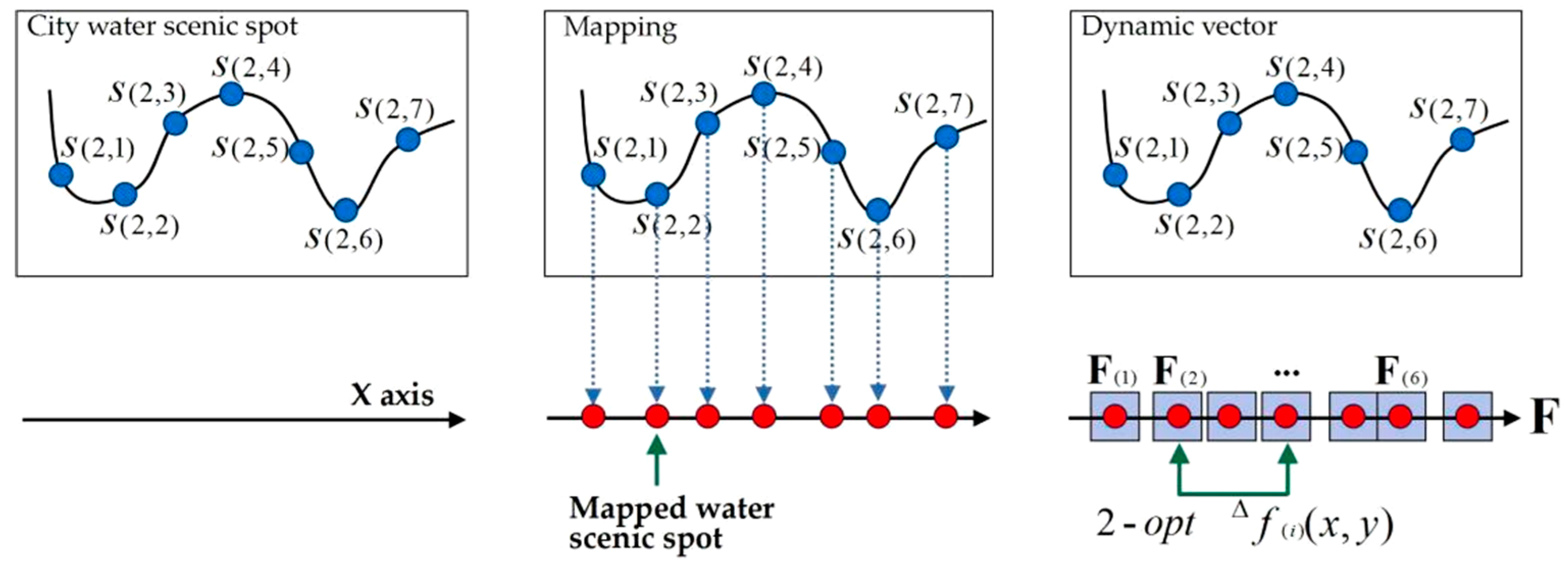
Tourist spatial decision-makingdynamic vector. The process of visitingnumber of scenic water spots, from the starting point, will form an integrated route. When the traveling sequence changes, the route will change too. In geographic space, the scenic water spots have spatial attributes. Map the scenic water spots on to a one-dimensional number axis, and form vector, to randomly store scenic water spots. The vector has the function ofdynamic operation. This vector is defined as the tourist spatial decision-makingdynamic vector.Figure 4shows the mapping process to form the vector. The vectormeets the following conditions:
- (1)
- The dimension is , the row rank is , and the column rank is ;
- (2)
- The first element of stores the starting point , and it is not involved in the algorithm;
- (3)
- From the second element to the No. element, they are used to store the number of scenic water spots ;
- (4)
- Arbitrary two elements and in the vectors can operate dynamic algorithm, .
Vector represents the tour sequence in the tourism spatial decision-making. When the scenic water spots are stored in the different elements in , they will form different tour routes, relating to different tourist spatial decision-making results. In the vector , the traveling cost between arbitrary elements and relates to the spatial decision-making section-cost function . One vector , formed by one arbitrary dynamic algorithm, relates to one spatial decision-making cost function .
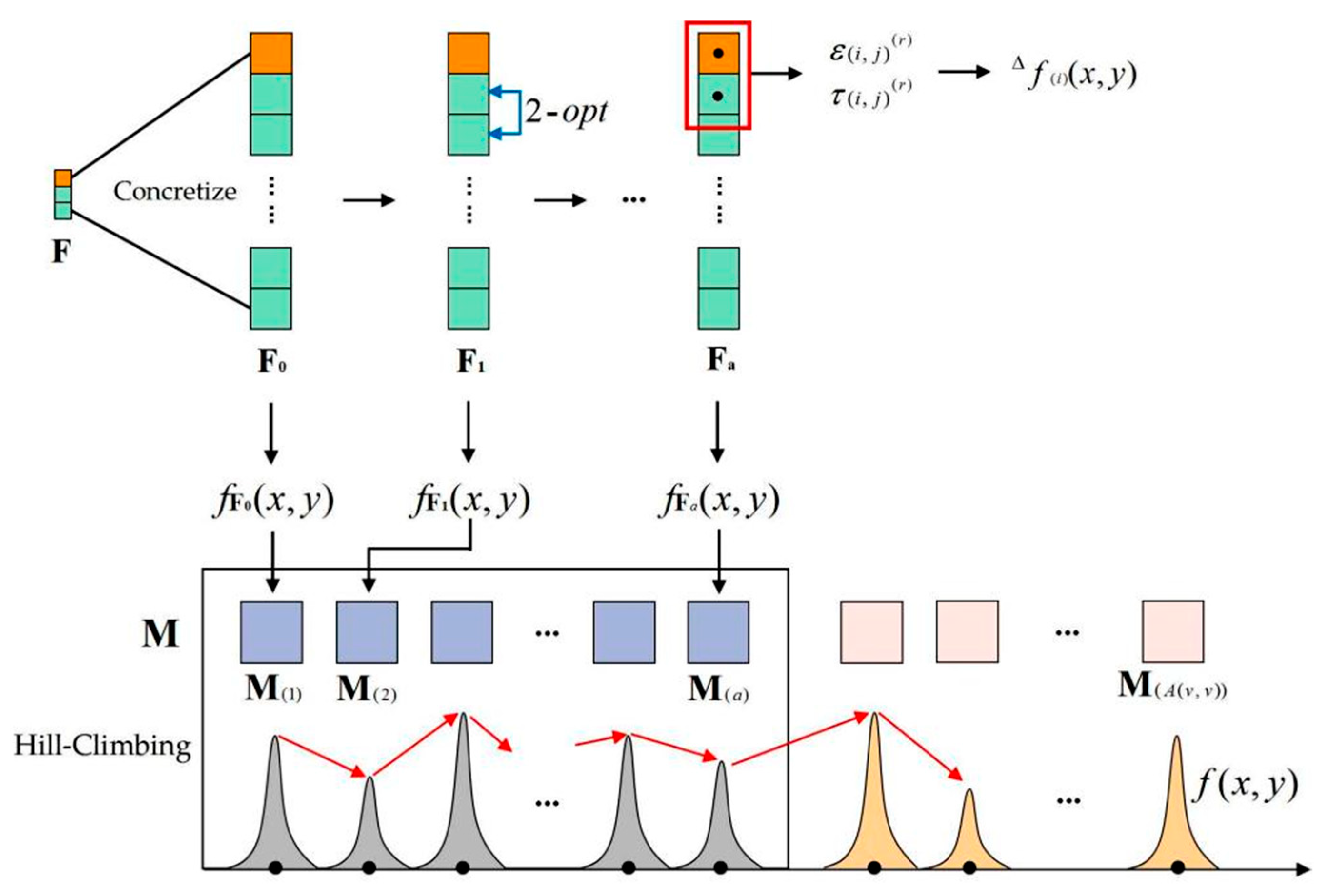
Definition 13.
Optimal peak value storage vector. When thedynamic algorithm is operated on the vector, it forms a new tour route. Each tour route relates to one spatial decision-making function. Traverse alldynamic operations for the vector, and generate all the feasible tour routes. Store the optimal tour routes with the cost functionintodimension vector; this vector is defined as the optimal peak-value storage vector. The vector is generated by the combination of thedynamic algorithm and the hill-climbing algorithm. The vectormeets the following conditions:
- (1)
- The dimension is , the row rank is , and the column rank is ;
- (2)
- In the process of the algorithm, the function values are dynamically stored, and the finally stored values are the optimal number of .
According to the above definitions and analysis, the decision-making algorithm for water-spot tourists, based on the spatial-accessibility optimization matrix, is constructed as follows. Figure 5 shows the spatial decision-making algorithm process for water-spot tourists, combined with the dynamic algorithm and the hill-climbing algorithm.
Input: Matrix . Tourists choose classifications , the number of the scenic water spots to be visited, the transportation modes .
Output: Vector .
Step 1: Based on , and , the system recommends the optimal scenic water spots in each and accumulates to the number ; Initialize , ;
Step 2: Confirm the starting point , store it in the No.1 element of . Randomly store the recommended number scenic water spots in the No.2 to No. elements , get the initialized vector .
Step 3: Based on the randomly chosen transportation mode in each road section, calculate the tourist spatial decision influence factor and the normalization factor for each section of scenic water spot and . Then calculate each section’s function value .
Step 4: Calculate , initialize the full ranked vector .
Sub-step 1: Calculate the of the initialized vector ; store the function value into No.1 element of ;
Sub-step 2: Perform the first dynamic algorithm on and get a new vector ; calculate the function value of the vector ; store the function value into No.2 element of ;
Sub-step 3: Perform the second dynamic algorithm on and get a new vector , judge:
- (1)
- If , calculate the of the vector , store the function value into No.3 element of ;
- (2)
- If , perform dynamic algorithm again.
Sub-step 4: In line with the method in sub-step 1~3, perform dynamic algorithm for number of times on , and each time it creates a different vector , store number of into vector and make the vector full-ranked. Create the peak-value graph for the vector .
Step 5: Continue the dynamic algorithm; do hill-climbing algorithm to search the optimal .
Sub-step 1: Perform the No. time of
dynamic algorithm on and get a new vector ; create the peak-function value graph for ; do hill-climbing algorithm:
- (1)
- If , delete the maximum peak value in current , store into vector ;
- (2)
- If , turn to Sub-step 2 and continue searching.
Sub-step 2: Perform the No. time of dynamic algorithm on and get a new vector ; create the peak-function value graph for , do hill-climbing algorithm:
- (1)
- If , delete the maximum peak value in current , store into vector ;
- (2)
- If , turn to Sub-step 3 and continue searching.
Sub-step 3: Perform the No. time of dynamic algorithm on , and get a new vector ; traverse ; create the peak-function value graph for ; do hill-climbing algorithm:
- (1)
- If , delete the maximum peak value in current , store into vector ;
- (2)
- If , continue searching until , the searching ends.
Step 6: Output the vector . The number of elements in are the number of minimum peak values in all of the number of peak values after the overall dynamic algorithm performances on .
As to the recommended vector with the minimum function peak values, the minimum value in relates to the tour route with the lowest costs, and the second-minimum value in relates to the tour route with the second-optimal costs. Based on the tourist’s schedule, the system recommends spatial decision-making schemes for the tourist.
3. Experiment, Results and Discussions
In order to verify that the proposed algorithm could effectively and reasonably provide spatial decision-making for water-spot tourists, an experiment was performed; then, the experimental results were analyzed and concluded. The basic process of the experiment was as follows. The research range was determined as the administrative area of Leshan city and the scenic water spots within the area; then, the decision-making influence factors and section-cost function values between the scenic water spots were calculated. The experiment compiled the previously visited scenic water spots and their classifications by the sample tourists, and classified the scenic water spots within the research range. After determining the starting point of the tour, the experiment analyzed the spatial accessibility of the scenic water spots, output the accessibility optimization matrix, and determined the scenic water spots to be visited with the optimal spatial accessibility, in accordance with the tourists’ needs in the scenic water spot classifications. Based on the choice of transportation modes by the tourists, the proposed algorithm was used to output the route with the minimum traveling costs, and then the experiment provided the tourists with the optimal spatial decision-making schemes.
3.1. Data Collection and Analysis of the Scenic Water-Spot Classification Results
- (1)
- The results of the experimental data collection.
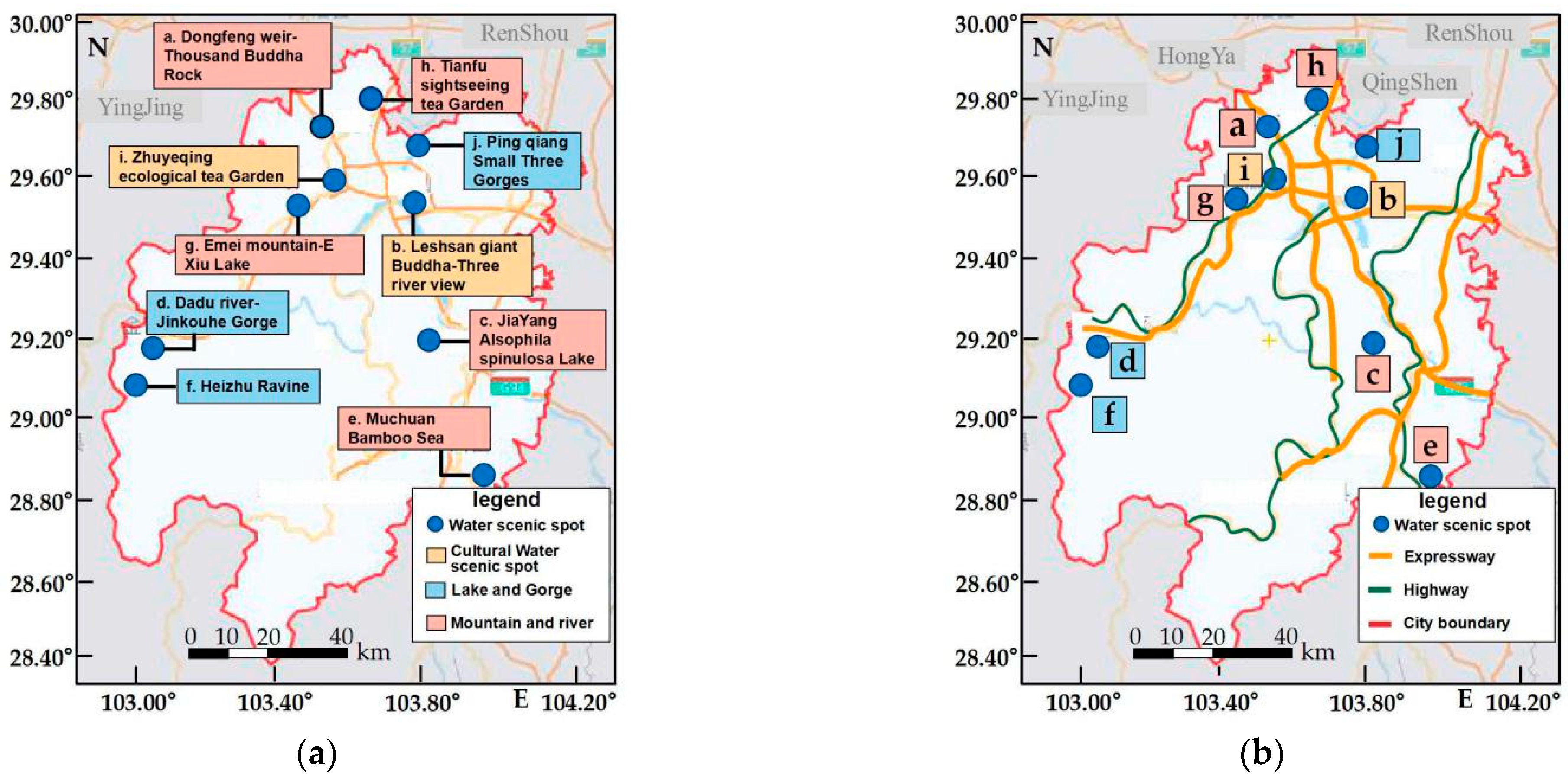
The experiment selected the tourist city of Leshan, and the scenic water spots within the administrative area as the research range and objects; the number was . The scenic water spots that the tourists had previously visited were compiled, and the number was . The feature-attributes of the scenic water spots were obtained from the tourism data website, and the feature-attribute vector for each scenic spot was established. The feature-attributes included : scenic water spot star rating (1–5 stars); : evaluation index (0~1.0); : ticket price (unit: yuan); : proper visiting-time duration (unit: h); : sightseeing; : humanity and history; : leisure and health care; : park and garden tour. The values ~ depended on whether the attribute existed in the scenic spot. If it existed, the value was 1; otherwise, it was 0. The feature-attribute distance for each scenic water spot in the research range was calculated, and their classifications were confirmed. The spatial-distribution data, of the scenic water spots in Leshan City and the main roads connecting the scenic water spots, were compiled, and it was supposed that the starting point of the sample tourist was Leshan high-speed railway station. Taking the starting point as the center, the data, on the road distances from the starting point to each scenic spot and the road distances between scenic spots, were collected. Meanwhile, under the conditions of travel by self-driving or by public bus, the driving mileage, traveling time and fee cost in each scenic-spot section, were compiled, and the spatial decision-making section cost function was calculated. Table 1 shows the classifications of the tourist’s previously visited scenic water spots, and the weighted values of the feature-attributes for each scenic water spot. Figure 6 shows the distribution of the scenic water spots and the main roads connecting the scenic water spots in Leshan City. Figure 6a shows the distribution of the scenic water spots. Different colors on the map annotation for the names of the scenic water spots in the figure represent different classifications: the orange color represents humanity scenic water spots; the blue color represents lakes and valleys; and the pink color represents mountains and rivers. Figure 6b shows the spatial road distribution around the scenic water spots.
- (2)
- The results of the scenic water-spot classification
Table 2 shows the classification results of the scenic water spots, and the weighted values of the feature attributes for each scenic water spot.
3.2. Calculation Results and Analysis of Scenic Water Spot Spatial Accessibility
- (1)
- The calculation results of the scenic water spot spatial accessibility.
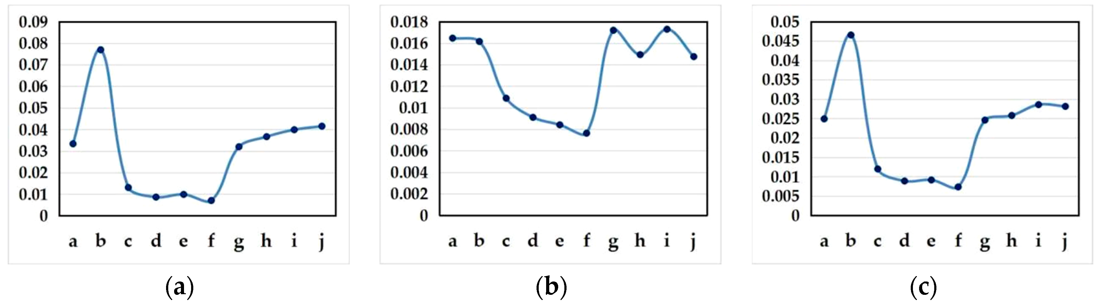
According to the spatial distribution of the starting point and the scenic water spots, and the road distances between the starting point and the scenic water spots, the road distances among the scenic water spots were used to calculate the starting-distance accessibility factor , the average traveling-distance accessibility factor and the weighted average accessibility factor , shown in Table 3. Through the factor calculation results, the spatial accessibility for each scenic water spot was obtained. Based on the Table 1 results, the scenic water-spot accessibility optimization matrix was output, as shown in Table 4. Based on the Table 3 data, the fluctuating curve graph of the starting-distance accessibility factor was output, as shown in Figure 7a. The fluctuating curve graph of the average traveling-distance accessibility factor was output, as shown in Figure 7b. The fluctuating curve graph of the weighted average accessibility factor was output, as shown in Figure 7c.
- (2)
- The discussions of the classification of the scenic water-spot spatial accessibility.
As regards the curves in Table 3 and Figure 7, different scenic water spots in the research range had different starting-distance accessibility factors, average traveling-distance accessibility factors and weighted average accessibility factors. (1) The scenic water spot with the maximum starting-distance accessibility factor was Leshan Giant Buddha–Three-River View, and the scenic water spot with the minimum starting-distance accessibility factor was Heizhugou Ravine, which indicated that the accessibility of Leshan Giant Buddha–Three-River View to the starting point was the strongest, and that the accessibility of Heizhugou Ravine to the starting point was the weakest. The higher the value of the starting-distance accessibility factor, the stronger was the accessibility of the scenic spot to the tourist’s starting point, and the easier it was for the tourist to get there. (2) The scenic water spot with the maximum average traveling-distance accessibility factor was Zhuyeqing Ecological Tea Garden, and the scenic water spot with the minimum average traveling-distance accessibility factor was Heizhugou Ravine, which indicated that Zhuyeqing Ecological Tea Garden had the strongest average accessibility among all the scenic spots. The accessibility from this scenic spot to the other ones was the strongest. Heizhugou Ravine had the weakest average accessibility among all the scenic spots, and the accessibility from this scenic spot to the other ones was the weakest. The higher the value of the average traveling-distance accessibility factor, the stronger was the average accessibility of the scenic spots to one another, and vice versa. (3) The scenic water spot with the maximum weighted average accessibility factor was Leshan Giant Buddha–Three-River View, and the scenic water spot with the minimum weighted average accessibility factor was Heizhugou Ravine, indicating that the comprehensive accessibility of Leshan Giant Buddha–Three-River View was the strongest, and that the comprehensive accessibility of Heizhugou Ravine was the weakest. The higher the value of the weighted average accessibility factor, the greater was the probability of being selected by the recommendation system, and then recommended to tourists in the same classification, and vice versa. Based on the data in Table 3, the starting-distance accessibility factors, the average traveling-distance accessibility factor and the weighted average accessibility factor of scenic water spots in Figure 7 all showed a fluctuating trend.
Analysis of the data in Table 4. In accordance with the results of the weighted average accessibility factor, the scenic water spots in the same classification were sequenced. As regards a given scenic water spot, the higher the value of the weighted average accessibility factor, the higher its ranking sequence was, and the greater was the probability of its being recommended to tourists. The scenic water spot ranked in the first element was preferentially recommended to tourists, then the second element, and so on.
3.3. The Comparison Analysis of the Water-Spot Tourist Spatial Decision-Making Results
- (1)
- The results of the water-spot tourist spatial decision-making.
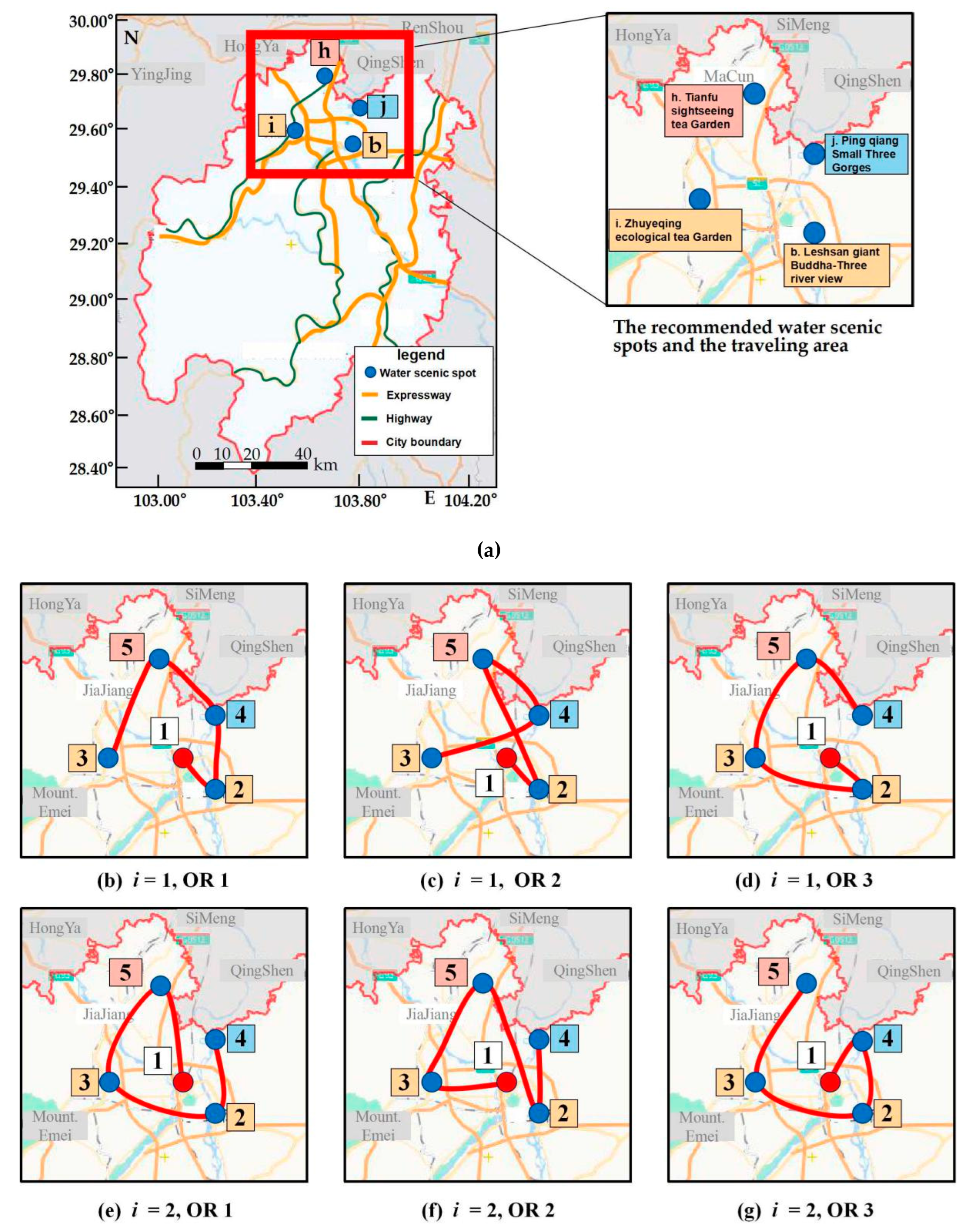
Based on the accessibility optimization matrix of scenic water spots in Table 4, the tourists chose the most-interested scenic water-spot classification according to needs and traveling schedule, and the system gave priority to recommending the scenic water spots with the highest accessibility-intensity for the tourists. The recommended results were Leshan Giant Buddha–Three-River View, Zhuyeqing Ecological Tea Garden, Pingqiang Small Three Gorges and Tianfu Sightseeing Tea Garden. According to the recommended results of the scenic water spots and the traveling-distance factor, time factor and cost factor between the scenic water spots under the condition of two transportation modes, the spatial decision-making section cost-function values between the scenic water spots were calculated, as shown in Table 4. The traveling-distance factor and time factor were compiled in an electronic map, the cost factor was calculated on the basis of a 7-liter self-driving car and the current average price of Leshan gasoline. The public transportation cost was calculated on the basis of the actual cost of taking tourist buses or city buses: namely, the fee for the bus ticket. Using the water-spot tourist spatial decision-making algorithm constructed in this study, the optimal route and two sub-optimal routes with the lowest cost, under the condition of two transportation modes, were output, and the total cost of the route was compared, as shown in Table 5: represents ‘self-driving’ and represents ‘public bus’; OR 1 represents the optimal route; OR 2 and OR 3 represent two sub-optimal routes; 1 represents the starting point—Leshan high-speed railway station; 2 represents the Leshan Giant Buddha–Three-River View scenic water spot; 3 represents the Zhuyeqing Ecological Tea Garden scenic water spot; 4 represents the Pingqiang Small Three Gorges scenic water spot; 5 represents the Tianfu Guanguang Tea Garden scenic water spot. The value in the ‘section cost function value’ column represents the cost between the scenic spots in the route, and the value in the ‘total cost’ column represents the total cost of the route. In the ‘cost difference’ column, the first value represents the total cost difference between OR 2 and OR 1, and the second value represents the total cost difference between OR 3 and OR 1. Figure 8 shows the spatial decision-making results of the optimal route and sub-optimal routes under the condition of two transportation modes; Figure 8a shows the extracted research range of the recommended scenic water spots; Figure 8b represents the optimal route for self-driving travel; Figure 8c,d represent the sub-optimal routes for self-driving travel; Figure 8e represents the optimal route for public bus travel; Figure 8f,g represent the sub-optimal routes for public bus travel. Thus, the system not only provided the tourists with spatial decision-making data, but also provided the tourists with visual results of the spatial decision-making schemes.
- (2)
- The discussions of the water-spot tourist spatial decision-making.
Comparison and analysis of the output routes: (1) when the tourists chose self-driving, the total cost of OR 1: 12453 was the lowest—that is: Leshan high-speed railway station—Leshan Giant Buddha–Three-River View—Pingqiang Small Three Gorges—Tianfu Sightseeing Tea Garden—Zhuyeqing Ecological Tea Garden. The total cost of the route was 4.7161, which was lower than other routes. In addition, OR 2: 12543 was the sub-optimal route—that is: Leshan high-speed railway station—Leshan Giant Buddha–Three-River View—Tianfu Sightseeing Tea Garden—Pingqiang Small Three Gorges—Zhuyeqing Ecological Tea Garden. The total cost of the route was 4.8794, which cost less for the tourists than any other routes, except for OR 1. Next, the route OR 3: 12354—namely: Leshan high-speed railway station—Leshan Giant Buddha–Three-River View—Zhuyeqing Ecological Tea Garden—Tianfu Sightseeing Tea Garden—Pingqiang Small Three Gorges. The total cost of the route was 4.9799, which cost less for the tourists than any other routes, except for OR 1 and OR 2. The cost function value of route OR 2 was 0.1633 higher than that of route OR 1, and the cost function value of route OR 3 was 0.2638 higher than that of route OR 1, indicating that among the three optimal routes, OR 1 had the lowest cost, followed by OR 2 and OR 3. When the tourists chose the decision-making route with the lowest cost to visit, it effectively reduced the energy consumption and the vehicle exhaust emissions to the environment. (2) When the tourists chose to travel by public bus, the total cost of OR 1: 15324 was the lowest—that is: Leshan high-speed railway station—Tianfu Sightseeing Tea Garden—Zhuyeqing Ecological Tea Garden—Leshan Giant Buddha–Three-River View—Pingqiang Small Three Gorges. The total cost of the route was 11.8800, which was lower than that of other routes. In addition, OR 2: 13524 was the sub-optimal route—that is: Leshan high-speed railway station—Zhuyeqing Ecological Tea Garden—Tianfu Sightseeing Tea Garden—Leshan Giant Buddha–Three River View—Pingqiang Small Three Gorges. The total cost of the route was 11.9080, which cost less for the tourists than any other routes, except for OR 1. Next, the route OR 3: 14235—that is: Leshan high-speed railway station—Pingqiang Small Three Gorges—Leshan Giant Buddha–Three River View—Zhuyeqing Ecological Tea Garden—Tianfu Sightseeing Tea Garden”. The total cost of the route was 12.2860, which cost less for the tourists than any other routes, except for OR 1 and OR 2. The cost function value of route OR 2 was 0.0280 higher than that of route OR 1, and route OR 3 was 0.4060 higher than that of route OR 1, indicating that among the three optimal routes, OR 1 had the lowest cost, followed by OR 2 and OR 3. When a tourist chose the decision-making route with the lowest cost to visit, it effectively reduced the energy consumption and the vehicle exhaust emissions to the environment.
According to the output optimal tour routes, the system provided the tourists with different spatial decision-making schemes. (1) When a tourist chose to travel by self-driving, the system proposed two-day and three-day traveling decision-making schemes on the route with the lowest cost OR 1: 12453. ① The first scheme was a two-day tour. The tourist arrived at Leshan high-speed railway station in the morning on the first day, drove to Leshan Giant Buddha and enjoyed the view of Giant Buddha and Three-Rivers. The sightseeing time was 2–3 h. In the afternoon, the tourist drove to Pingqiang Small Three Gorges, took a cruise to enjoy the beautiful scenery of Minjiang River, and obtained accommodation in Pingqiang Small Three Gorges at night. The next morning, the tourist drove to Tianfu Sightseeing Tea Garden, visited the tea mountain and enjoyed the lake scenery. In the afternoon, the tourist drove to the Zhuyeqing Ecological Tea Garden, visited the tea garden and tasted the Zhuyeqing green tea. The trip ended in the evening. ② The second scheme was a three-day tour. The tourist arrived at Leshan high-speed railway station on the first day, took the public bus to Tianfu Sightseeing Tea Garden, visited the tea mountain and enjoyed the lake scenery. In the afternoon, the tourist took a bus to Zhuyeqing Ecological Tea Garden, visited the tea garden, tasted Zhuyeqing green tea, returned to Leshan in the evening and obtained accommodation. The next day, the tourist took a public bus to Leshan Giant Buddha, enjoyed the view of the Giant Buddha and Three-Rivers, participated in a night tour of Three-River View in the evening, enjoyed the Giant Buddha and Leshan night scenery, and obtained accommodation in Leshan. On the third day, the tourist took a bus to Pingqiang Small Three Gorges, took a cruise to enjoy the beautiful scenery of Minjiang River, and returned to Leshan in the evening.
3.4. Results and Discussions
The main achievements and contributions of the study were as follows. Firstly, unlike traditional tourism decision-making methods, in this study, tourists’ interests and tendencies were obtained by the attributes knowledge-mined from the scenic water spots that the tourists had previously visited, on the basis of which, the scenic water spots in the tourism destination city were classified. By this method, the recommended scenic water spots could best match the tourists’ interests. Secondly, the existing studies on the recommendation system lacked the spatial attributes of the recommended objects. This study proposed a method to set up a scenic water-spot spatial accessibility model, and conducted research on the scenic water-spot spatial accessibility, which was used as an important and necessary condition for recommending scenic spots, planning tour routes and performing tourist decision-makings. Thirdly, the study on spatial accessibility was used for tour route planning and tourist spatial decision-making, which conformed to the spatial attributes of tourism activities and the actual conditions of traveling; it could provide theoretical and technical support for the development of a tourism recommendation system, a tour route planning system and a tourist spatial decision-making system. Fourthly, the methods constructed in the study could provide references for further research on tourist spatial accessibility, a tourist recommendation algorithm and a tour route planning algorithm, etc. The aims of the study also included travel-cost savings and reducing energy consumption. Thus, in regard to low-carbon tourism and green traveling, this study provides a new research method.
4. Conclusions
This study proposes a low-carbon decision-making algorithm for water-spot tourists, based on the k-NN spatial-accessibility optimization model. An optimization model based on k-NN accessibility was constructed, to confirm the scenic water-spot interest classifications and tourists’ interest-tendencies. Then, the scenic water spot spatial-accessibility optimization model was constructed, and the study of scenic water-spot spatial accessibility was used in the tourist spatial decision-making, based on the tour route planning algorithm. In the experiment, the results of tourist spatial decision-making, under different transportation modes, were obtained and concluded. By comparing the optimal tour route with the sub-optimal tour routes, it can be concluded that the optimal tour route had stronger spatial accessibility and lower cost consumption. When tourists chose the optimal tour route for sightseeing, it effectively saved traveling costs, and produced the lowest energy consumption and vehicle exhaust emissions, thus realizing low-carbon and environmentally friendly travel.
The spatial decision-making method for water-spot tourists, constructed in this study, was based on tourists’ preferences for previously visited scenic water spots, and the spatial research range was the administrative area of a tourist city, including its urban districts and outskirts counties. In future research, we will conduct further studies on the following two aspects. Firstly, we will design a more detailed interest-mining algorithm for scenic water spots, propose indexes with more complete classifications, diverse types and comprehensive coverage of tourists’ interest-tendencies, and design quantitative methods for each indicator. Through the in-depth mining of tourists’ interest-tendencies, tourists’ requirements for scenic water spots will be accurately confirmed. Secondly, we will further expand the research range, take the provincial administrative area as the research object, study the spatial distribution and spatial accessibility of scenic water spots in a broader scope, integrate more cross-region transportation modes, and provide tourists with a wider range of traveling decisions.
Author Contributions
Conceptualization, X.Z. and B.W.; methodology, X.Z. and B.W.; validation and formal analysis, M.S. and J.T.; investigation, data resources and data processing, X.Z. and J.T.; writing—original draft preparation, X.Z.; writing—review and editing, X.Z., B.W. and M.S.; visualization, M.S. and J.T.; supervision, X.Z.; project administration and funding acquisition, B.W. and X.Z. All authors have read and agreed to the published version of the manuscript.
Funding
This research was funded by the National Natural Science Foundation of China (Grant No. 42101455), the Humanities and Social Sciences Project of Sichuan Provincial Department of Education (Guo Moruo Research, Grant No. GY2022C01) and the Leshan Science and Technology Plan Project (Grant No. 22RKX0029).
Institutional Review Board Statement
Not applicable.
Informed Consent Statement
Not applicable.
Data Availability Statement
The data presented in this study are available from the author upon reasonable request.
Acknowledgments
The authors would like to thank the Postdoctoral Innovation Practice Base of the Sichuan province of Leshan Vocational and Technical College, and the Computer Science Postdoctoral Mobile Station of Sichuan University. We thank the editors and reviewers for their valuable comments.
Conflicts of Interest
The authors declare no conflict of interest.
Abbreviations
| Abbreviation | Definition |
| Element of scenic water-spot classification training set | |
| Scenic water-spot initial training set | |
| Scenic water-spot classification | |
| Scenic water-spot classification training set | |
| The to-be-classified scenic water-spot element | |
| Scenic water-spot classification matrix. | |
| Scenic water-spot feature attribute | |
| Feature-attribute vector | |
| Feature-attribute normalization parameter | |
| k-NN element feature distance | |
| Starting-distance accessibility factor | |
| Average traveling-distance accessibility factor | |
| The weighted average accessibility factor | |
| Scenic water spot accessibility optimization matrix | |
| Tourism spatial decision influence factor | |
| Normalization factor | |
| Spatial decision-making section cost function | |
| Spatial decision-making cost function | |
| Tourism spatial decision-making dynamic vector | |
| Optimal peak-value storage vector |
References
- Hu, J.L.; Ai, Y.; Zheng, W.J.; Tian, M.Y. A Research on the Accessibility of Traditional Villages in Guilin Based on Space Syntax. J. Xi’an Univ. Archit. Technol. 2022, 41, 38–46. [Google Scholar]
- Ou’yang, J.; Chen, S.J.; Wang, D. Layout of China Tourism Airports Based on the Spatial Accessibility of Important Scenic Spots. China Trans. Outlook 2021, 43, 21–26. [Google Scholar]
- Wang, C.; Li, X.D.; Kong, L.Z.; Li, Z.S.; Wang, S.M. Study on Tourism Competitiveness and Spatial Development Strategy of Cities along Lan-Xin High-speed Railway. J. Northwest Norm. Univ. 2021, 57, 33–39. [Google Scholar]
- Gong, Y.X.; Ji, X.; Zhang, Y. Study on the Optimization of Tourism Transportation System of Urban and Rural Settlements in Water Network Area—A Case Study of Jinhu County. J. Nanjing Norm. Univ. 2020, 43, 45–52. [Google Scholar]
- Sun, G.X. Symmetry Analysis in Analyzing Cognitive and Emotional Attitudes for Tourism Consumers by Applying Artificial Intelligence Python Technology. Symmetry 2020, 12, 606. [Google Scholar] [CrossRef]
- Gu, Z.H.; Zhang, Y.; Chen, Y.; Chang, X.M. Analysis of Attraction Features of Tourism Destinations in a Mega-City Based on Check-in Data Mining—A Case Study of Shenzhen, China. ISPRS Int. J. Geo-Inf. 2016, 5, 210. [Google Scholar] [CrossRef]
- Wang, L.; Li, S.; Liu, Q.H. Study on Spatial Distribution Feature and Accessibility of A-level Scenic Spots in Ganzi Prefecture. Anhui Agric. Sci. Bull. 2021, 27, 183–185. [Google Scholar]
- Xu, S.Y.; Xie, J.A.; Liu, M.J.; Cheng, M.Y. Spatial Characteristics and Correlation Analysis of Road Time Accessibility to Tourist Attractions in Qinghai Province. Highway 2022, 6, 222–228. [Google Scholar]
- Yang, Y.B.; Deng, Q. Study on the Spatial Distribution Pattern and Highway Accessibility of Red Villages in Hunan Province. Resour. Environ. Yangtze Basin 2022, 31, 793–804. [Google Scholar]
- Dong, X.; Qiao, Q.; Zhai, L.; Sun, L.; Zhen, Y. Evaluating the Accessibility of Plaza Park Using the Gravity Model. J. Geo-Inf. Sci. 2019, 21, 1518–1526. [Google Scholar]
- Li, X.Y.; Wang, X.F.; Zhuo, R.R.; Wan, L.X. Spatial Accessibility of Leisure Agriculture in Suburbs of Wuhan based on spatial syntax and network analysis. J. Ctrl. China Norm. Univ. 2020, 54, 882–891. [Google Scholar]
- Wang, L.; Cao, X.S.; Hu, L.L. Research on the Impact of Tourist Attractions Accessibility on Tourist Flow in Different Travel Times: A Case Study of Xi’an City. Human Geogr. 2021, 3, 157–165. [Google Scholar]
- Luo, H.F. Analysis and Optimization of Traffic Accessibility of Scenic Spots in Lushan Scenic Spot. Master’s Thesis, Jiangxi Science and Technology Normal University, Nanchang, China, 2021. [Google Scholar]
- Yang, G.M.; Yang, Y.R.; Gong, G.F.; Gui, Q.Q. The Spatial Network Structure of Tourism Efficiency and Its Influencing Factors in China: A Social Network Analysis. Sustainability 2022, 14, 9921. [Google Scholar] [CrossRef]
- Włodarczyk, B.; Cudny, W. Individual Low-Cost Travel as a Route to Tourism Sustainability. Sustainability 2022, 14, 10514. [Google Scholar] [CrossRef]
- Bagunaid, W.; Chilamkurti, N.; Veeraraghavan, P. AISAR: Artificial Intelligence-Based Student Assessment and Recommendation System for E-Learning in Big Data. Sustainability 2022, 14, 10551. [Google Scholar] [CrossRef]
- Wang, H.M.; Wei, X.J.; Ao, W.X. Assessing Park Accessibility Based on a Dynamic Huff Two-Step Floating Catchment Area Method and Map Service API. ISPRS Int. J. Geo-Inf. 2022, 11, 394. [Google Scholar] [CrossRef]
- Horak, J.; Kukuliac, P.; Maresova, P.; Orlikova, L.; Kolodziej, O. Spatial Pattern of the Walkability Index, Walk Score and Walk Score Modification for Elderly. ISPRS Int. J. Geo-Inf. 2022, 11, 279. [Google Scholar] [CrossRef]
- Raza, A.; Zhong, M.; Safdar, M. Evaluating Locational Preference of Urban Activities with the Time-Dependent Accessibility Using Integrated Spatial Economic Models. Int. J. Environ. Res. Public Health 2022, 19, 8317. [Google Scholar] [CrossRef]
- Xu, H.; Zhao, J. Planning Urban Internal Transport Based on Cell Phone Data. Appl. Sci. 2022, 12, 8433. [Google Scholar] [CrossRef]
- Mehrian, M.R.; Miandoab, A.M.; Abedini, A.; Aram, F. The Impact of Inefficient Urban Growth on Spatial Inequality of Urban Green Resources (Case Study: Urmia City). Resources 2022, 11, 62. [Google Scholar] [CrossRef]
- Bajwoluk, T.; Langer, P. Impact of the “Krakow East-Bochnia” Road Transport Corridor on the Form of the Functio-Spatial Structure and Its Economic Activity. Sustainability 2022, 14, 8281. [Google Scholar] [CrossRef]
- Liu, J.; Zhou, G.; Linderholm, H.W.; Song, Y.; Liu, D.-L.; Shen, Y.; Liu, Y.; Du, J. Optimal Strategy on Radiation Estimation for Calculating Universal Thermal Climate Index in Tourism Cities of China. Int. J. Environ. Res. Public Health 2022, 19, 8111. [Google Scholar] [CrossRef] [PubMed]
- Grübel, J.; Thrash, T.; Aguilar, L.; Gath-Morad, M.; Chatain, J.; Sumner, R.W.; Hölscher, C.; Schinazi, V.R. The Hitchhiker’s Guide to Fused Twins: A Review of Access to Digital Twins In Situ in Smart Cities. Remote Sens. 2022, 14, 3095. [Google Scholar] [CrossRef]
- Chang, X.L.; Huang, X.Y.; Jiang, X.C.; Xiao, R. Impacts of Transportation Networks on the Landscape Patterns—A Case Study of Shanghai. Remote Sens. 2022, 14, 4060. [Google Scholar] [CrossRef]
- Guo, Q.H.; He, Z.C.; Li, D.W.; Spyra, M. Analysis of Spatial Patterns and Socioeconomic Activities of Urbanized Rural Areas in Fujian Province, China. Land 2022, 11, 969. [Google Scholar] [CrossRef]
- Tsushima, H.; Matsuura, T.; Ikeguchi, T. Searching Strategies with Low Computational Costs for Multiple-Vehicle Bike Sharing System Routing Problem. Appl. Sci. 2022, 12, 2675. [Google Scholar] [CrossRef]
- Santos, B.; Passos, S.; Gonçalves, J.; Matias, I. Spatial Multi-Criteria Analysis for Road Segment Cycling Suitability Assessment. Sustainability 2022, 14, 9928. [Google Scholar] [CrossRef]
- Zheng, X.; Luo, Y.; Sun, L.; Yu, Q.; Zhang, J.; Chen, S. A Novel Multi-Objective and Multi-Constraint Route Recommendation Method Based on Crowd Sensing. Appl. Sci. 2021, 11, 10497. [Google Scholar] [CrossRef]
- Sajid, M.; Singh, J.; Haidri, R.A.; Prasad, M.; Varadarajan, V.; Kotecha, K.; Garg, D. A Novel Algorithm for Capacitated Vehicle Routing Problem for Smart Cities. Symmetry 2021, 13, 1923. [Google Scholar] [CrossRef]
- Ma, X.F.; Tan, J.X.; Zhang, J.K. Spatial-Temporal Correlation between the Tourist Hotel Industry and Town Spatial Morphology: The Case of Phoenix Ancient Town, China. Sustainability 2022, 14, 10577. [Google Scholar] [CrossRef]
- Damos, M.A.; Zhu, J.; Li, W.; Hassan, A.; Khalifa, E. A Novel Urban Tourism Path Planning Approach Based on a Multiobjective Genetic Algorithm. ISPRS Int. J. Geo-Inf. 2021, 10, 530. [Google Scholar] [CrossRef]
- Khamsing, N.; Chindaprasert, K.; Pitakaso, R.; Sirirak, W.; Theeraviriya, C. Modified ALNS Algorithm for a Processing Application of Family Tourist Route Planning: A Case Study of Buriram in Thailand. Computation 2021, 9, 23. [Google Scholar] [CrossRef]
- Ruan, L.; Kou, X.; Ge, J.; Long, Y.; Zhang, L. A Method of Directional Signs Location Selection and Content Generation in Scenic Areas. ISPRS Int. J. Geo-Inf. 2020, 9, 574. [Google Scholar] [CrossRef]
- Chen, J. Title Research on the Optimization of Tourist Traffic Routes in Beijing, Tianjin and Hebei Province Starting form Beijing and Tianjin. Tianjin Soc. Inst. 2019, 2, 71–81. [Google Scholar]
- Sun, Y.; Liu, S.; Li, L. Grey Correlation Analysis of Transportation Carbon Emissions under the Background of Carbon Peak and Carbon Neutrality. Energies 2022, 15, 3064. [Google Scholar] [CrossRef]
- Zhang, S.L. Evaluation of Accessibility of the Tourism Node and Study on Optimization of Tour-Routes in Hebei Province. Master’s Thesis, Hebei Normal University, Shijiazhuang, China, May 2015. [Google Scholar]
- Chen, J.X. Optimization of Tourism Routes in Northern Anhui Based on Dijkstra. J. Luoyang Inst. Sci. Technol. 2014, 24, 55–57. [Google Scholar]
- Bao, J.; Lu, L.; Ji, Z.H. Tourism transportation optimization and tour route designing of north Anhui province based on the Kruskal algorithm of graph-theory. Human Geogr. 2010, 25, 144–148. [Google Scholar]
Figure 1.
The flow diagram of the methodology in this study.

Figure 2.
The modeling process of the scenic water-spot classification algorithm, based on k-NN mining.
Figure 2.
The modeling process of the scenic water-spot classification algorithm, based on k-NN mining.

Figure 3.
The modeling process of the scenic water spot accessibility optimization matrix .

Figure 4.
The process by which to form the vector from the scenic water-spot mapping.

Figure 5.
Spatial decision-making algorithm for water-spot tourists process, combined with dynamic algorithm and hill-climbing algorithm.
Figure 5.
Spatial decision-making algorithm for water-spot tourists process, combined with dynamic algorithm and hill-climbing algorithm.

Figure 6.
The distribution of the scenic water spots, and the main roads connecting scenic water spots in Leshan City: (a) shows the distribution of the scenic water spots. Different colors on the map annotation for the names of scenic water spots in the figure represent different classifications; the orange color represents humanity scenic water spots; the blue color represents lakes and valleys; and the pink color represents mountains and rivers; (b) shows the spatial distribution of the roads around the scenic water spots.

Figure 7.
The fluctuating curve graph of the accessibility factors for the scenic water spots: (a) the fluctuating curve graph of the starting-distance accessibility factor ; (b) the fluctuating curve graph of the average traveling-distance accessibility factor ; (c) the fluctuating curve graph of the weighted average accessibility factor . Scenic water spots in the table: a. Dongfeng Weir–Thousand Buddha Rock; b. Leshan Giant Buddha–Three-River View; c. JiaYang Alsophila Spinulosa Lake; d. Dadu River–Jinkouhe Gorge; e. Muchuan Bamboo Sea; f. Heizhu Ravine; g. Emei Mountain–E Xiu Lake; h. Tianfu Sightseeing Tea Garden; i. Zhuyeqing Ecological Tea Garden; j. Ping Qiang Small Three Gorges.

Figure 8.
Spatial decision-making results for the optimal route and sub-optimal routes under the two different transportation modes. (a) shows the extracted research range of the recommended scenic water spots; (b) represents the optimal route for self-driving travel; (c,d) represent the sub-optimal routes for self-driving travel; (e) represents the optimal route for public bus travel; (f,g) represent the sub-optimal routes for public bus travel.


Table 1.
The classifications of the tourists’ previously visited scenic water spots, and the weighted values of the feature attributes for each scenic water spot.
Table 1.
The classifications of the tourists’ previously visited scenic water spots, and the weighted values of the feature attributes for each scenic water spot.
| Previously Visited Water Scenic | |||||||||
|---|---|---|---|---|---|---|---|---|---|
| Humanity scenic water spot | The Summer Palace | 0.50 | 0.94 | 0.30 | 0.30 | 1.00 | 1.00 | 0.00 | 1.00 |
| Suzhou Gardens | 0.50 | 0.92 | 0.80 | 0.20 | 0.00 | 1.00 | 0.00 | 1.00 | |
| Guangzhou Chimelong | 0.50 | 0.96 | 2.50 | 0.80 | 0.00 | 0.00 | 0.00 | 1.00 | |
| Yu Garden, Shanghai | 0.40 | 0.94 | 0.40 | 0.20 | 0.00 | 1.00 | 0.00 | 1.00 | |
| Tang Paradise | 0.50 | 0.88 | 0.00 | 0.20 | 1.00 | 1.00 | 0.00 | 1.00 | |
| Baotu Spring | 0.50 | 0.9 | 0.40 | 0.20 | 1.00 | 1.00 | 0.00 | 1.00 | |
| Lakes and valleys | Qiandao Lake | 0.50 | 0.88 | 1.20 | 0.50 | 1.00 | 0.00 | 1.00 | 0.00 |
| Qinglong Lake–Sansheng Flower Town | 0.40 | 0.78 | 0.00 | 0.40 | 1.00 | 0.00 | 1.00 | 0.00 | |
| Xinyang Nanwan Lake | 0.40 | 0.82 | 0.60 | 0.20 | 1.00 | 0.00 | 1.00 | 0.00 | |
| West Lake | 0.50 | 0.94 | 0.00 | 0.20 | 1.00 | 1.00 | 1.00 | 0.00 | |
| Qinghai Lake | 0.50 | 0.92 | 0.00 | 0.20 | 1.00 | 0.00 | 1.00 | 0.00 | |
| Mountains and rivers | Zhengzhou Yellow River Tourist Area | 0.40 | 0.84 | 0.60 | 0.30 | 1.00 | 1.00 | 1.00 | 1.00 |
| Juzhou Park–Xiangjiang River scenery | 0.50 | 0.90 | 0.00 | 0.20 | 1.00 | 0.00 | 1.00 | 0.00 | |
| Tengwangge–Ganjiang River scenery | 0.50 | 0.90 | 0.50 | 0.20 | 1.00 | 1.00 | 0.00 | 0.00 | |
| Longmen Grottoes–Yihe River scenery | 0.50 | 0.92 | 0.90 | 0.20 | 1.00 | 1.00 | 0.00 | 1.00 | |
| Huangguoshu Waterfall | 0.50 | 0.9 | 1.80 | 0.30 | 1.00 | 0.00 | 1.00 | 0.00 | |
| Xiaolangdi of the Yellow River | 0.40 | 0.86 | 0.40 | 0.20 | 1.00 | 1.00 | 0.00 | 1.00 | |
| Du Fu thatched cottage–Huanhua Creek | 0.40 | 0.92 | 0.50 | 0.20 | 1.00 | 1.00 | 0.00 | 1.00 |
Table 2.
The classification results of the scenic water spots in the research range, and the weighted values of the feature attributes for each scenic water spot.
Table 2.
The classification results of the scenic water spots in the research range, and the weighted values of the feature attributes for each scenic water spot.
| Classification Name | Scenic Water Spot in the Research Range | ||||||||
|---|---|---|---|---|---|---|---|---|---|
| Humanity water scenic spot | Leshan Giant Buddha—Three-River View | 0.50 | 0.90 | 0.80 | 0.30 | 1.00 | 1.00 | 1.00 | 1.00 |
| Zhuyeqing Ecological Tea Garden | 0.30 | 0.86 | 0.20 | 0.20 | 0.00 | 0.00 | 1.00 | 1.00 | |
| Lakes and valleys | Ping Qiang Small Three Gorges | 0.10 | 0.88 | 0.00 | 0.30 | 1.00 | 0.00 | 1.00 | 0.00 |
| Dadu River–Jinkouhe Gorge | 0.40 | 0.88 | 0.00 | 0.30 | 1.00 | 0.00 | 1.00 | 0.00 | |
| Heizhu Ravine | 0.40 | 0.88 | 0.48 | 0.30 | 1.00 | 0.00 | 1.00 | 0.00 | |
| Mountains and rivers | Tianfu Sightseeing Tea Garden | 0.40 | 0.88 | 0.30 | 0.20 | 1.00 | 0.00 | 1.00 | 1.00 |
| Dongfeng Weir–Thousand Buddha Rock | 0.40 | 0.88 | 0.50 | 0.20 | 1.00 | 1.00 | 1.00 | 1.00 | |
| Emei Mountain–E Xiu Lake | 0.50 | 0.92 | 1.60 | 0.30 | 1.00 | 1.00 | 1.00 | 0.00 | |
| JiaYang Alsophila Spinulosa Lake | 0.40 | 0.80 | 1.00 | 0.20 | 1.00 | 1.00 | 1.00 | 0.00 | |
| Muchuan Bamboo Sea | 0.30 | 0.90 | 0.39 | 0.20 | 1.00 | 0.00 | 1.00 | 0.00 |
Table 3.
The calculated starting-distance accessibility factor λ(1), the average traveling-distance accessibility factor λ(2) and the weighted average accessibility factor λ(3). Scenic water spots in the table: a. Dongfeng Weir–Thousand Buddha Rock; b. Leshan Giant Buddha–Three-River View; c. JiaYang Alsophila Spinulosa Lake; d. Dadu River–Jinkouhe Gorge; e. Muchuan Bamboo Sea; f. Heizhu Ravine; g. Emei Mountain–E Xiu Lake; h. Tianfu Sightseeing Tea Garden; i. Zhuyeqing Ecological Tea Garden; j. Ping Qiang Small Three Gorges.
| Scenic Water Spot | a | b | c | d | e |
| 0.0333 | 0.0769 | 0.0131 | 0.0086 | 0.0099 | |
| 0.0165 | 0.0161 | 0.0109 | 0.0091 | 0.0084 | |
| 0.0249 | 0.0465 | 0.0120 | 0.0089 | 0.0091 | |
| Scenic Water Spot | f | g | h | i | j |
| 0.0070 | 0.0319 | 0.0366 | 0.0398 | 0.0415 | |
| 0.0076 | 0.0172 | 0.0149 | 0.0173 | 0.0147 | |
| 0.0073 | 0.0246 | 0.0258 | 0.0286 | 0.0281 |
Table 4.
Scenic water-spot accessibility optimization matrix. Scenic water spots in the table: a. Dongfeng Weir–Thousand Buddha Rock; b. Leshan Giant Buddha–Three-River View; c. JiaYang Alsophila Spinulosa Lake; d. Dadu River–Jinkouhe Gorge; e. Muchuan Bamboo Sea; f. Heizhu Ravine; g. Emei Mountain–E Xiu Lake; h. Tianfu Sightseeing Tea Garden; i. Zhuyeqing Ecological Tea Garden; j. Ping Qiang Small Three Gorges.
| Classification Name | Classification Results | Weighted Average Accessibility Factor | Sequence of Spatial Accessibility Intensity |
|---|---|---|---|
| Humanity scenic water spot | b | 0.0465 | 1 |
| i | 0.0286 | 2 | |
| Lakes and valleys | j | 0.0281 | 1 |
| d | 0.0089 | 2 | |
| f | 0.0073 | 3 | |
| Mountains and rivers | h | 0.0258 | 1 |
| a | 0.0249 | 2 | |
| g | 0.0246 | 3 | |
| c | 0.0120 | 4 | |
| e | 0.0091 | 5 |
Table 5.
Optimal route and sub-optimal routes, section cost function value, total cost result comparison and the cost different comparison under the two transportation modes.
Table 5.
Optimal route and sub-optimal routes, section cost function value, total cost result comparison and the cost different comparison under the two transportation modes.
| Transportation Mode | Tour Route | Section Cost Function Value | Total Cost | Cost Difference | |||
| OR 1: 12453 | 0.6907 | 1.4863 | 1.1408 | 1.3983 | 4.7161 | ||
| OR 2: 12543 | 0.6907 | 1.5062 | 1.1408 | 1.5416 | 4.8794 | 0.1633 | |
| OR 3: 12354 | 0.6907 | 1.7500 | 1.3983 | 1.1408 | 4.9799 | 0.2638 | |
| Transportation mode | Tour Route | Section cost function value | Total cost | Cost difference | |||
| OR 1: 15324 | 1.9970 | 3.6020 | 3.3420 | 2.9390 | 11.8800 | ||
| OR 2: 13524 | 1.5630 | 3.6020 | 3.8040 | 2.9390 | 11.9080 | 0.0280 | |
| OR 3: 14235 | 2.4030 | 2.9390 | 3.3420 | 3.6020 | 12.2860 | 0.4060 | |
Publisher’s Note: MDPI stays neutral with regard to jurisdictional claims in published maps and institutional affiliations. |
© 2022 by the authors. Licensee MDPI, Basel, Switzerland. This article is an open access article distributed under the terms and conditions of the Creative Commons Attribution (CC BY) license (https://creativecommons.org/licenses/by/4.0/).
Share and Cite
MDPI and ACS Style
Zhou, X.; Wen, B.; Su, M.; Tian, J. A Low-Carbon Decision-Making Algorithm for Water-Spot Tourists, Based on the k-NN Spatial-Accessibility Optimization Model. Water 2022, 14, 2920. https://doi.org/10.3390/w14182920
AMA Style
Zhou X, Wen B, Su M, Tian J. A Low-Carbon Decision-Making Algorithm for Water-Spot Tourists, Based on the k-NN Spatial-Accessibility Optimization Model. Water. 2022; 14(18):2920. https://doi.org/10.3390/w14182920
Chicago/Turabian StyleZhou, Xiao, Bowei Wen, Mingzhan Su, and Jiangpeng Tian. 2022. "A Low-Carbon Decision-Making Algorithm for Water-Spot Tourists, Based on the k-NN Spatial-Accessibility Optimization Model" Water 14, no. 18: 2920. https://doi.org/10.3390/w14182920
Note that from the first issue of 2016, this journal uses article numbers instead of page numbers. See further details here.