

Spatiotemporal Characteristics and Influencing Factors of Water Resources’ Green Utilization Efficiency in China: Based on the EBM Model with Undesirable Outputs and SDM Model
 , ,
, ,
Abstract
:1. Introduction
2. Data and Methods
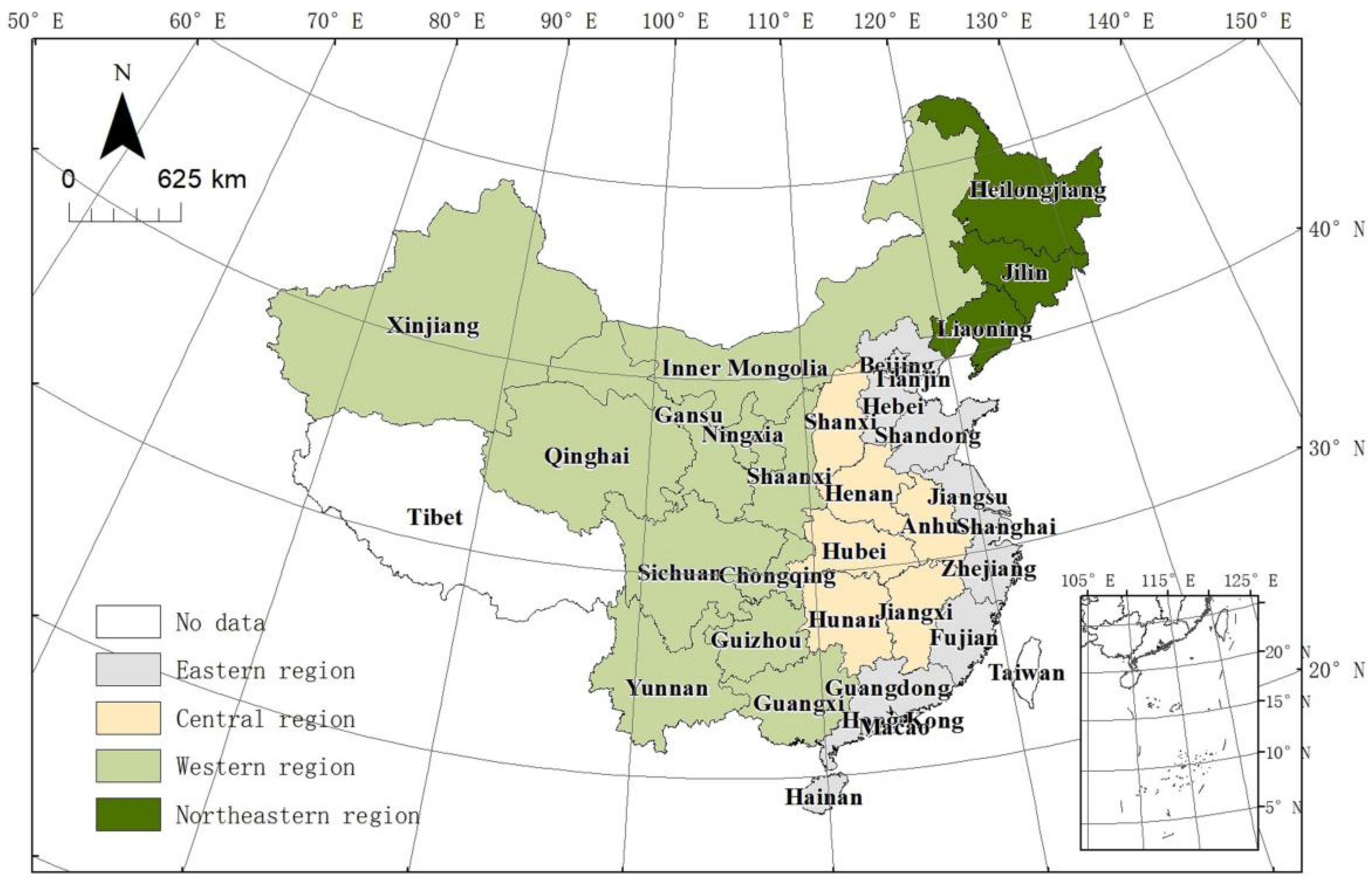
2.1. Research Area
2.2. Index Selection and Data Sources
WSGUE Assessment Indicators
- (1)
- Input indicators. We selected the total water consumption, employee index, and capital stock as input indicators. The total water consumption, including agricultural, industrial, domestic, and ecological water, referred to the data from NBSC [2]. The employee data came from the statistical yearbook of the Chinese provinces (2010–2020) [27].
- (2)
- The capital stock was estimated through the perpetual inventory method in this paper. According to Zhang et al. [28], the depreciation rate registered at 9.6%, and the capital stock in 2009 was equal to the investment in fixed assets divided by 10%. The price indices of the investment in fixed assets were converted to 2009 prices based in accordance with China Fixed Capital Investment Yearbook (2010–2013, 2015–2018) [29], China Investment Statistical Bulletin (2014) [30], China Investment Statistical Yearbook (2019–2020) [31], and NBSC [2].
- (3)
- The desirable output indicator. Gross regional product (GDP) was selected as the desirable output indicator in this paper. The provincial GDP was converted to 2009 prices based on GDP deflator. Relevant data were obtained from NBSC [2].
- (4)
- The undesirable output indicators. COD and nitrogen emissions from wastewater were selected, which have been the key monitored objects by the related department of environmental management in China for a long time, which are selected as two undesirable output indicators.
2.3. Driving Factors of WRGUE
2.3.1. Economic Development Level
2.3.2. Water Resources Utilization Structure
2.3.3. Technical Progress
2.3.4. Opening-Up Policy
2.3.5. Urbanization
2.3.6. Population Density
2.4. Methods
2.4.1. The EBM Model with Undesirable Outputs
2.4.2. Spatial Autocorrelation Analysis
2.4.3. Spatial Durbin Model
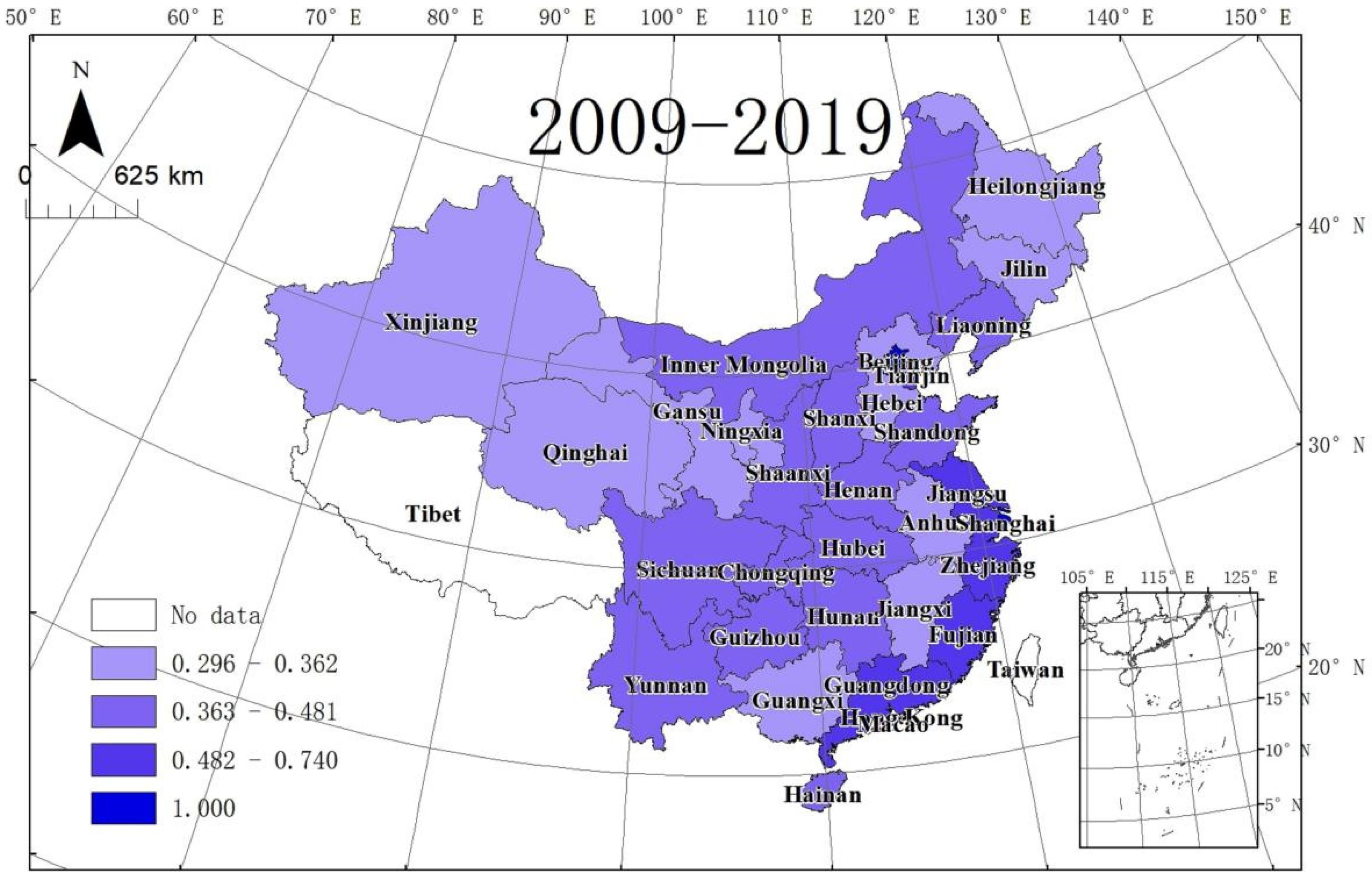
3. Results
4. Discussions
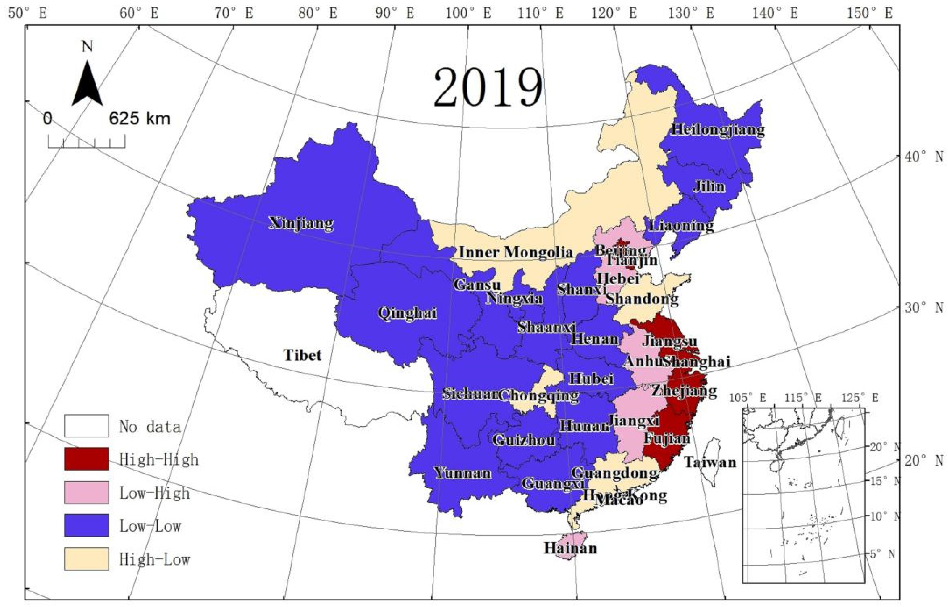
4.1. Spatial Autocorrelation Analysis of WRGUE
4.2. Discussion on Influencing Factors for of WRGUE
5. Conclusions
Author Contributions
Funding
Institutional Review Board Statement
Informed Consent Statement
Data Availability Statement
Conflicts of Interest
References
- Zhou, X.; Luo, R.; Yao, L.; Cao, S.; Wang, S.; Lev, B. Assessing integrated water use and wastewater treatment systems in China: A mixed network structure two-stage SBM DEA model. J. Clean. Prod. 2018, 185, 533–546. [Google Scholar] [CrossRef]
- National Bureau of Statistics of China. China Statistical Yearbooks (CSY) (2009–2018); China Statistical Publishing House: Beijing, China, 2009–2018. Available online: http://tongji.oversea.cnki.net/oversea/engnavi/HomePage.aspx?id=N2017100312&name=YINFN&floor=1 (accessed on 29 August 2022).
- Jiang, Y. China’s water security: Current status, emerging challenges and future prospects. Environ. Sci. Policy 2015, 54, 106–125. [Google Scholar] [CrossRef]
- Li, W.; Zuo, Q.; Jiang, L.; Zhang, Z.; Ma, J.; Wang, J. Evaluation of Regional Water Resources Management Performance and Analysis of the Influencing Factors: A Case Study in China. Water 2022, 14, 574. [Google Scholar] [CrossRef]
- Song, M.; Wang, R.; Zeng, X. Water resources utilization efficiency and influence factors under environmental restrictions. J. Clean. Prod. 2018, 184, 611–621. [Google Scholar] [CrossRef]
- Deng, G.; Li, L.; Song, Y. Provincial water use efficiency measurement and factor analysis in China: Based on SBM-DEA model. Ecol. Indicat. 2016, 69, 12–18. [Google Scholar] [CrossRef]
- Yi, W.; Liu, L.Y. Evolution of water-use efficiency in the Yangtze River Economic Belt based on national strategies and water environment treatment. Ecol. Inform. 2022, 69, 101642. [Google Scholar] [CrossRef]
- Li, D.; Shi, H.; Ma, P.; Zhu, S.; Xu, H. Understanding the Mechanism of Urbanization Affect Agricultural Water Efficiency: Evidence from China. Water 2022, 14, 2176. [Google Scholar] [CrossRef]
- Zhou, Q.; Tong, C. Does Rapid Urbanization Improve Green Water-Use Efficiency? Based on the Investigation of Guangdong Province, China. Sustainability 2022, 14, 7481. [Google Scholar] [CrossRef]
- Gong, Z.; He, Y.; Chen, X. Evaluation of Regional Water Use Efficiency under Green and Sustainable Development Using an Improved Super Slack-Based Measure Model. Sustainability 2022, 14, 7149. [Google Scholar] [CrossRef]
- Wei, J.; Lei, Y.; Yao, H.; Ge, J.; Wu, S.; Liu, L. Estimation and influencing factors of agricultural water efficiency in the Yellow River basin, China. J. Clean. Prod. 2021, 308, 127249. [Google Scholar] [CrossRef]
- Grassauer, F.; Herndl, M.; Nemecek, T.; Guggenberger, T.; Fritz, C.; Steinwidder, A.; Zollitsch, W. Eco-efficiency of farms considering multiple functions of agriculture: Concept and results from Austrian farms. J. Clean. Prod. 2021, 297, 126662. [Google Scholar] [CrossRef]
- Xie, Q.; Xu, Q.; Rao, K.; Dai, Q. Water pollutant discharge permit allocation based on DEA and non-cooperative game theory. J. Environ. Manag. 2022, 302, 113962. [Google Scholar] [CrossRef] [PubMed]
- Liu, K.; Yang, G.; Yang, D. Investigating industrial water-use efficiency in mainland China: An improved SBM-DEA model. J. Environ. Manag. 2020, 270, 110859. [Google Scholar] [CrossRef] [PubMed]
- Dhehibi, B.; Lachaal, L.; Elloumi, M.; Messaoud, E.B. Measuring irrigation water use efficiency using stochastic production frontier: An application on citrus producing farms in Tunisia. Afr. J. Agric. Resour. Econ. 2007, 1, 1–15. [Google Scholar]
- Phillips, M.A. Inefficiency in Japanese water utility firms: A stochastic frontier approach. J. Regul. Econ. 2013, 44, 197–214. [Google Scholar] [CrossRef]
- Kaneko, S.; Tanaka, K.; Toyota, T.; Managi, S. Water efficiency of agricultural production in China: Regional comparison from 1999 to 2002. Int. J. Agric. Resour. Gov. Ecol. 2004, 3, 231–251. Available online: http://www.inderscience.com/link.php?id=6038 (accessed on 31 August 2022). [CrossRef]
- Battes, G.E.; Coelli, T.J. Model for Technical in Efficiency Effects in a Stochastic Production Frontier for Panel Data. Empir. Econ. 1995, 20, 325–332. [Google Scholar] [CrossRef]
- Cullinane, K.; Wang, T.F.; Song, D.W.; Ji, P. The Technical Efficiency of Container Ports: Comparing Data Envelopment Analysis and Stochastic Frontier Analysis. Transp. Res. Part A 2006, 40, 354–374. Available online: https://kns.cnki.net/kns/brief/default_result.aspx (accessed on 31 August 2022). [CrossRef]
- Tone, K.; Tsutsui, M. An epsilon-based measure of efficiency in DEA: A third pole of technical efficiency. Eur. J. Oper. Res. 2010, 207, 1554–1563. [Google Scholar] [CrossRef]
- Tao, X.; Wang, P.; Zhu, B. Provincial Green Economics Efficiency of China: A non-separable input-output SBM approach. Appl. Energy 2016, 171, 58–66. [Google Scholar] [CrossRef]
- Yang, L.; Wang, K.L.; Geng, J.C. China’s regional ecological energy efficiency and energy saving and pollution abatement potentials: An empirical analysis using epsilon-based measure model. J. Clean. Prod. 2018, 194, 300–308. [Google Scholar] [CrossRef]
- Zeng, L. China’s Eco-Efficiency: Regional Differences and Influencing Factors Based on a Spatial Panel Data Approach. Sustainability 2021, 13, 3143. [Google Scholar] [CrossRef]
- Zhao, P.; Zeng, L.; Li, P.; Lu, H.; Hu, H.; Li, C.; Zheng, M.; Li, H.; Yu, Z.; Yuan, D.; et al. China’s transportation sector carbon dioxide emissions efficiency and its influencing factors based on the EBM DEA model with undesirable outputs and spatial Durbin model. Energy 2022, 238, 121934. [Google Scholar] [CrossRef]
- Zeng, L.; Lu, H.; Liu, Y.; Zhou, Y.; Hu, H. Analysis of Regional Differences and Influencing Factors on China’s Carbon Emission Efficiency in 2005–2015. Energies 2019, 12, 3081. [Google Scholar] [CrossRef]
- Ren, Y.F.; Fang, C.L.; Li, G.D. Spatiotemporal characteristics and influential factors of eco-efficiency in Chinese prefecture-level cities: A spatial panel econometric analysis. J. Clean. Prod. 2020, 260, 120787. [Google Scholar] [CrossRef]
- All Province Bureaus of Statistics of China. All Provincial Statistical Yearbooks, 2010–2018. Available online: https://tongji.cnki.net/kns55/Navi/NaviDefault.aspx (accessed on 29 August 2022).
- Zhang, J.; Wu, G.Y.; Zhang, J.P. The Estimation of China’s Provincial Capital Stock: 1952–2000. Econ. Res. J. 2004, 10, 35–44. Available online: http://en.cnki.com.cn/Article_en/CJFDTOTAL-JJYJ200410004.htm (accessed on 29 August 2022).
- National Bureau of Statistics of China. China Fixed Capital Investment Yearbook, 2010–2013, 2015–2018; National Bureau of Statistics of China: Beijing, China, 2010–2013, 2015–2018. Available online: https://data.cnki.net/yearbook/Single/N2019030174 (accessed on 29 August 2022).
- National Bureau of Statistics of China. China Investment Statistical Bulletin, 2014; National Bureau of Statistics of China: Beijing China, 2014. Available online: https://bbs.pinggu.org/thread-8356048-1-1.html (accessed on 29 August 2022).
- National Bureau of Statistics of China. China Investment Statistical Yearbook, 2019–2020; National Bureau of Statistics of China: Beijing, China, 2019–2020. Available online: https://data.cnki.net/yearbook/Single/N2022010278 (accessed on 29 August 2022).
- Bao, C.; Chen, X. Spatial econometric analysis on influencing factors of water consumption efficiency in urbanizing China. J. Geogr. Sci. 2017, 27, 1450–1462. [Google Scholar] [CrossRef]
- Zheng, J.; Zhang, H.; Xing, Z. Re-Examining Regional Total-Factor Water Efficiency and Its Determinants in China: A Parametric Distance Function Approach. Water 2018, 10, 1286. [Google Scholar] [CrossRef]
- Zhang, W.; Wang, D.; Liu, X. Does financial agglomeration promote the green efficiency of water resources in China? Environ. Sci. Pollut. Res. 2021, 28, 56628–56641. [Google Scholar] [CrossRef]
- Yang, Q.; Liu, H.J. Water Resources Performance in China under the Constraint on Pollution Emissions: Dynamic Trend and Driving Factors. J. Financ. Econ. 2015, 41, 56628–56641. Available online: https://xueshu.baidu.com/usercenter/paper/show?paperid=072fc248f27fabc007abd065b1127a66 (accessed on 29 August 2022).
- Liu, G.; Najmuddin, O.; Zhang, F. Evolution and the drivers of water use efficiency in the water-deficient regions: A case study on Ω-shaped Region along the Yellow River, China. Environ. Sci. Pollut. Res. 2022, 29, 19324–19336. [Google Scholar] [CrossRef] [PubMed]
- Charnes, A.; Cooper, W.W.; Rhodes, E. Measuring the Efficiency of Decision Making Units. Eur. J. Oper. Res. 1978, 2, 429–444. [Google Scholar] [CrossRef]
- Banker, R.D.; Charnes, A.; Cooper, W.W. Some models for estimating technical and scale inefficiencies in data envelopment analysis. Manag. Sci. 1984, 30, 1078–1092. [Google Scholar] [CrossRef] [Green Version]
- Tone, K. Slacks-based measure of efficiency in data envelopment analysis. Eur. J. Oper. Res. 2001, 130, 498–509. [Google Scholar] [CrossRef]
- Zeng, L. The Driving Mechanism of Urban Land Green Use Efficiency in China Based on the EBM Model with Undesirable Outputs and the Spatial Dubin Model. Int. J. Environ. Res. Public Health 2022, 19, 10748. [Google Scholar] [CrossRef]
- Ning, L.; Zheng, W.; Zeng, L. Research on China’s Carbon Dioxide Emissions Efficiency from 2007 to 2016: Based on Two Stage Super Efficiency SBM Model and Tobit Model. Acta Sci. Nat. Univ. Pekin. 2021, 57, 181–188. Available online: https://www.scopus.com/inward/record.uri?eid=2-s2.0-85101373648&doi=10.13209%2fj.0479-8023.2020.111&partnerID=40&md5=d948ef3627771ac2ca544cbf07fbc229 (accessed on 29 August 2022).
- Zhao, P.J.; Zeng, L.E.; Lu, H.Y.; Zhou, Y.; Hu, H.Y.; Wei, X.Y. Green economic efficiency and its influencing factors in China from 2008 to 2017: Based on the super-SBM model with undesirable outputs and spatial Dubin model. Sci. Total Environ. 2020, 741, 140026. [Google Scholar] [CrossRef]
- Tobler, W.R. A computer movie simulating urban growth in the Detroit region. Econ. Geogr. 1970, 46, 234–240. [Google Scholar] [CrossRef]
- Li, C.; Shi, H.; Zeng, L.; Dong, X. How Strategic Interaction of Innovation Policies between China’s Regional Governments Affects Wind Energy Innovation. Sustainability 2022, 14, 2543. [Google Scholar] [CrossRef]
- Zeng, L.; Li, C.; Liang, Z.; Zhao, X.; Hu, H.; Wang, X.; Yuan, D.; Yu, Z.; Yang, T.; Lu, J.; et al. The Carbon Emission Intensity of Industrial Land in China: Spatiotemporal Characteristics and Driving Factors. Land 2022, 11, 1156. [Google Scholar] [CrossRef]
- Zeng, L.; Li, H.; Wang, X.; Yu, Z.; Hu, H.; Yuan, X.; Zhao, X.; Li, C.; Yuan, D.; Gao, Y.; et al. China’s Transport Land: Spatiotemporal Expansion Characteristics and Driving Mechanism. Land 2022, 11, 1147. [Google Scholar] [CrossRef]
- Yang, W.Y.; Wang, W.L.; Ouyang, S.S. The influencing factors and spatial spillover effects of CO2 emissions from transportation in China. Sci. Total Environ. 2019, 696, 133900. [Google Scholar] [CrossRef] [PubMed]
- Lesage, J.P.; Pace, P.K. Introduction to Spatial Econometrics; CRC Press Taylor & Francis Group: New York, NY, USA, 2009. [Google Scholar]
- Lu, H.; Zhao, P.; Dong, Y.; Hu, H.; Zeng, L. Accessibility of high-speed rail stations and spatial disparity of urban-rural income gaps. Prog. Geogr. 2022, 41, 131–142. Available online: http://www.progressingeography.com/CN/Y2022/V41/I1/131 (accessed on 29 August 2022). [CrossRef]
- Elhorst, J.P. Spatial Panel Data Models. In Spatial Econometrics; SpringerBriefs in Regional Science; Springer: Berlin/Heidelberg, Germany, 2014. [Google Scholar] [CrossRef]
- Jenks, G.F. The data model concept in statistical mapping. Int. Yearb. Cartogr. 1967, 7, 186–190. Available online: https://xueshu.baidu.com/usercenter/paper/show?paperid=3a917c675547e8306d705d50ee3c73a6 (accessed on 29 August 2022).
- Yan, Z.; Zhou, W.; Wang, Y.; Chen, X. Comprehensive Analysis of Grain Production Based on Three-Stage Super-SBM DEA and Machine Learning in Hexi Corridor, China. Sustainability 2022, 14, 8881. [Google Scholar] [CrossRef]
- Zhao, P.; Lyu, D.; Hu, H.; Cao, Y.; Xie, J.; Pang, L.; Zeng, L.; Zhang, T.; Yuan, D. Population-development oriented comprehensive modern transport system in China. Acta Geogr. Sin. 2020, 75, 2699–2715. Available online: https://www.scopus.com/inward/record.uri?eid=2-s2.0-85098962061&doi=10.11821%2fdlxb202012011&partnerID=40&md5=270e79cdb27ca6f57cde65fc25170846 (accessed on 29 August 2022).
- Zeng, L.; Li, H.; Lao, X.; Hu, H.; Wei, Y.; Li, C.; Yuan, X.; Guo, D.; Liu, K. China’s Road Traffic Mortality Rate and Its Empirical Research from Socio-Economic Factors Based on the Tobit Model. Systems 2022, 10, 122. [Google Scholar] [CrossRef]
- The Department of Economic and Social Affairs. The Sustainable Development Goals Report 2021; United Nations Publications: New York, NY, USA, 2021; Available online: https://unstats.un.org/sdgs/report/2021/goal-06/ (accessed on 29 August 2022).


| Primary Indicators | Specific Indicators | Mean | Min | Max |
|---|---|---|---|---|
| Input indicators | The total water consumption (108 tons) | 201.1952 | 22.5 | 619.1 |
| The capital stock (RMB 108 Yuan) | 130,946.5 | 7982.3 | 530,575 | |
| The social employee (104 person) | 2719.8 | 303.26 | 7150.25 | |
| Desirable output indicator | GDP (RMB 108 Yuan) | 19,083.8 | 939.7 | 87,731.7 |
| Undesirable output indicator | The COD of wastewater (104 tons) | 50.62 | 1.97 | 198.3 |
| The nitrogen of wastewater (104 tons) | 5.06 | 0.1 | 23.09 |
| Explanatory Variable | Variables’ Definition and Unit | Pre-Judgment |
|---|---|---|
| Economic development level | Per capita GDP (RMB 104 Yuan) | Positive |
| Water resources use structure | Proportion of agricultural water to the total water consumption (%) | Negative |
| Technical progress level | Proportion of R& D expenditure to GDP (%) | Positive |
| Opening-up level | Proportion of the foreign trade to GDP (%) | Positive |
| Urbanization level | Proportion of the urban population to the total resident (%) | Unknown |
| Population density | Resident population per square kilometer (person/sq.km) | Unknown |
| Fixed Effects | Random Effects | |
|---|---|---|
| Wald test spatial lag | 46.56 *** | 112.08 *** |
| LR test spatial lag | 42.80 *** | 80.20 *** |
| Wald test spatial error | 27.99 *** | 53.92 *** |
| LR test spatial error | 34.12 *** | 77.79 *** |
| InDEL | InWSUS | InTDL | InOPL | InUL | InPD | Mean VIF | |
|---|---|---|---|---|---|---|---|
| VIF | 5.44 | 1.74 | 3.32 | 2.76 | 5.81 | 3.47 | 3.76 |
| 1/VIF | 0.184 | 0.575 | 0.301 | 0.362 | 0.172 | 0.288 |
| Regions | 2009 | 2010 | 2011 | 2012 | 2013 | 2014 | 2015 | 2016 | 2017 | 2018 | 2019 | Mean |
|---|---|---|---|---|---|---|---|---|---|---|---|---|
| Beijing | 1.000 | 1.000 | 1.000 | 1.000 | 1.000 | 1.000 | 1.000 | 1.000 | 1.000 | 1.000 | 1.000 | 1.000 |
| Tianjing | 0.581 | 0.595 | 0.629 | 0.584 | 0.656 | 0.666 | 0.610 | 1.004 | 0.555 | 0.627 | 0.595 | 0.646 |
| Hebei | 0.387 | 0.381 | 0.384 | 0.352 | 0.382 | 0.368 | 0.355 | 0.368 | 0.332 | 0.336 | 0.331 | 0.362 |
| Shanghai | 1.000 | 1.000 | 1.000 | 1.000 | 1.000 | 1.000 | 1.000 | 1.000 | 1.000 | 1.000 | 1.000 | 1.000 |
| Jiangsu | 0.558 | 0.567 | 0.575 | 0.539 | 0.605 | 0.620 | 0.607 | 0.681 | 0.561 | 0.580 | 0.548 | 0.586 |
| Zhejiang | 0.635 | 0.641 | 0.639 | 0.571 | 0.636 | 0.623 | 0.598 | 0.632 | 0.548 | 0.571 | 0.558 | 0.605 |
| Fujian | 0.571 | 0.579 | 0.562 | 0.507 | 0.562 | 0.541 | 0.509 | 0.550 | 0.473 | 0.470 | 0.456 | 0.525 |
| Shandong | 0.495 | 0.490 | 0.486 | 0.454 | 0.496 | 0.495 | 0.474 | 0.501 | 0.454 | 0.469 | 0.472 | 0.481 |
| Guangdong | 0.819 | 0.823 | 0.792 | 0.692 | 0.794 | 0.775 | 0.722 | 0.802 | 0.661 | 0.648 | 0.610 | 0.740 |
| Hainan | 0.447 | 0.459 | 0.445 | 0.386 | 0.422 | 0.400 | 0.367 | 0.385 | 0.329 | 0.319 | 0.305 | 0.388 |
| Eastern region | 0.649 | 0.653 | 0.651 | 0.609 | 0.655 | 0.649 | 0.624 | 0.692 | 0.591 | 0.602 | 0.588 | 0.633 |
| Shanxi | 0.443 | 0.436 | 0.441 | 0.402 | 0.436 | 0.415 | 0.379 | 0.375 | 0.355 | 0.368 | 0.362 | 0.401 |
| Anhui | 0.352 | 0.361 | 0.359 | 0.335 | 0.363 | 0.355 | 0.336 | 0.382 | 0.324 | 0.315 | 0.306 | 0.344 |
| Jiangxi | 0.336 | 0.339 | 0.334 | 0.314 | 0.340 | 0.335 | 0.321 | 0.331 | 0.301 | 0.297 | 0.287 | 0.321 |
| Henan | 0.417 | 0.422 | 0.433 | 0.392 | 0.440 | 0.438 | 0.415 | 0.443 | 0.383 | 0.390 | 0.376 | 0.414 |
| Hubei | 0.467 | 0.475 | 0.474 | 0.428 | 0.471 | 0.457 | 0.427 | 0.467 | 0.400 | 0.390 | 0.378 | 0.439 |
| Hunan | 0.444 | 0.453 | 0.452 | 0.404 | 0.451 | 0.439 | 0.408 | 0.435 | 0.382 | 0.371 | 0.355 | 0.418 |
| Central region | 0.410 | 0.414 | 0.415 | 0.379 | 0.417 | 0.406 | 0.381 | 0.405 | 0.358 | 0.355 | 0.344 | 0.390 |
| Inner Mongolia | 0.393 | 0.397 | 0.398 | 0.374 | 0.419 | 0.410 | 0.402 | 0.476 | 0.403 | 0.441 | 0.432 | 0.413 |
| Guangxi | 0.357 | 0.352 | 0.354 | 0.314 | 0.348 | 0.336 | 0.310 | 0.330 | 0.275 | 0.264 | 0.246 | 0.317 |
| Chongqing | 0.396 | 0.414 | 0.440 | 0.423 | 0.471 | 0.474 | 0.467 | 0.640 | 0.478 | 0.535 | 0.516 | 0.478 |
| Sichuan | 0.370 | 0.383 | 0.404 | 0.370 | 0.415 | 0.404 | 0.380 | 0.407 | 0.366 | 0.364 | 0.355 | 0.383 |
| Guizhou | 0.431 | 0.431 | 0.433 | 0.383 | 0.425 | 0.403 | 0.371 | 0.382 | 0.325 | 0.310 | 0.292 | 0.381 |
| Yunnan | 0.413 | 0.414 | 0.412 | 0.374 | 0.419 | 0.401 | 0.376 | 0.415 | 0.354 | 0.344 | 0.328 | 0.386 |
| Shaanxi | 0.397 | 0.405 | 0.419 | 0.396 | 0.429 | 0.424 | 0.406 | 0.423 | 0.390 | 0.404 | 0.401 | 0.408 |
| Gansu | 0.369 | 0.365 | 0.361 | 0.319 | 0.354 | 0.336 | 0.307 | 0.353 | 0.287 | 0.286 | 0.278 | 0.329 |
| Qinghai | 0.333 | 0.331 | 0.334 | 0.311 | 0.325 | 0.308 | 0.288 | 0.293 | 0.278 | 0.276 | 0.270 | 0.304 |
| Ningxia | 0.326 | 0.321 | 0.322 | 0.293 | 0.317 | 0.309 | 0.295 | 0.315 | 0.278 | 0.276 | 0.264 | 0.301 |
| Xinjiang | 0.409 | 0.400 | 0.394 | 0.337 | 0.377 | 0.362 | 0.327 | 0.343 | 0.284 | 0.279 | 0.262 | 0.343 |
| Western region | 0.381 | 0.383 | 0.388 | 0.354 | 0.391 | 0.379 | 0.357 | 0.398 | 0.338 | 0.344 | 0.331 | 0.368 |
| Liaoning | 0.385 | 0.388 | 0.398 | 0.373 | 0.408 | 0.403 | 0.398 | 0.453 | 0.389 | 0.404 | 0.402 | 0.400 |
| Jilin | 0.289 | 0.291 | 0.290 | 0.283 | 0.309 | 0.306 | 0.291 | 0.328 | 0.289 | 0.291 | 0.283 | 0.296 |
| Heilongjiang | 0.388 | 0.384 | 0.373 | 0.324 | 0.356 | 0.344 | 0.321 | 0.355 | 0.302 | 0.296 | 0.286 | 0.339 |
| Northeast | 0.354 | 0.354 | 0.354 | 0.327 | 0.358 | 0.351 | 0.337 | 0.379 | 0.327 | 0.330 | 0.324 | 0.345 |
| China | 0.474 | 0.477 | 0.478 | 0.441 | 0.481 | 0.472 | 0.449 | 0.496 | 0.425 | 0.431 | 0.418 | 0.458 |
| Year | Global Moran’s I | Z-Score | p-Value |
|---|---|---|---|
| 2009 | 0.224 ** | 2.249 | 0.025 |
| 2010 | 0.237 ** | 2.355 | 0.019 |
| 2011 | 0.247 ** | 2.446 | 0.014 |
| 2012 | 0.231 ** | 2.375 | 0.018 |
| 2013 | 0.251 ** | 2.465 | 0.014 |
| 2014 | 0.263 *** | 2.567 | 0.010 |
| 2015 | 0.254 ** | 2.522 | 0.012 |
| 2016 | 0.297 *** | 2.775 | 0.006 |
| 2017 | 0.208 ** | 2.158 | 0.031 |
| 2018 | 0.236 ** | 2.362 | 0.018 |
| 2019 | 0.225 *** | 2.294 | 0.022 |
| Spatial Fixed-Effects | Time Fixed-Effects | Spatial and Time Fixed-Effects | |
|---|---|---|---|
| InDEL | 0.8086419 *** | 0.7220803 *** | 0.6974106 *** |
| InWSUS | 0.0004369 | −0.0032236 | −0.0004647 |
| InTDL | 0.0937041 *** | 0.0039324 | 0.0824482 ** |
| InOPL | 0.0625741 *** | 0.0125481 | 0.0717951 *** |
| InUL | −0.9996273 *** | −0.2393367 *** | −0.9468609 *** |
| InPD | −0.0295799 | 0.1158211 *** | −0.1191172 |
| W*InDEL | −0.8510972 *** | −0.4911258 *** | −1.53070 *** |
| W*InWSUS | −0.0068093 | −0.0752403 *** | 0.0045217 |
| W*InTDL | −0.0155968 | −0.1458118 ** | 0.014417 |
| W*InOPL | −0.0166994 | 0.1628485 *** | 0.0597447 * |
| W*InUL | 0.9070408 *** | −0.0868307 | 1.122323 *** |
| W*InPD | −0.3018763 | −0.0216836 | −0.9419549 *** |
| Variance sigma2_e | 0.0030164 *** | 0.0136224 *** | 0.0024756 *** |
| R-squared | 0.3562 | 0.0010 | 0.2760 |
| Log-likelihood | 472.5766 | 240.4700 | 521.8122 |
Publisher’s Note: MDPI stays neutral with regard to jurisdictional claims in published maps and institutional affiliations. |
© 2022 by the authors. Licensee MDPI, Basel, Switzerland. This article is an open access article distributed under the terms and conditions of the Creative Commons Attribution (CC BY) license (https://creativecommons.org/licenses/by/4.0/).
Share and Cite
Zeng, L.; Li, P.; Yu, Z.; Nie, Y.; Li, S.; Gao, G.; Huang, D. Spatiotemporal Characteristics and Influencing Factors of Water Resources’ Green Utilization Efficiency in China: Based on the EBM Model with Undesirable Outputs and SDM Model. Water 2022, 14, 2908. https://doi.org/10.3390/w14182908
Zeng L, Li P, Yu Z, Nie Y, Li S, Gao G, Huang D. Spatiotemporal Characteristics and Influencing Factors of Water Resources’ Green Utilization Efficiency in China: Based on the EBM Model with Undesirable Outputs and SDM Model. Water. 2022; 14(18):2908. https://doi.org/10.3390/w14182908
Chicago/Turabian StyleZeng, Liangen, Peilin Li, Zhao Yu, Yang Nie, Shengzhang Li, Guangye Gao, and Di Huang. 2022. "Spatiotemporal Characteristics and Influencing Factors of Water Resources’ Green Utilization Efficiency in China: Based on the EBM Model with Undesirable Outputs and SDM Model" Water 14, no. 18: 2908. https://doi.org/10.3390/w14182908