
Biomathematical Model for Water Quality Assessment: Macroinvertebrate Population Dynamics and Dissolved Oxygen
 ,
,  , , and
Abstract
:1. Introduction
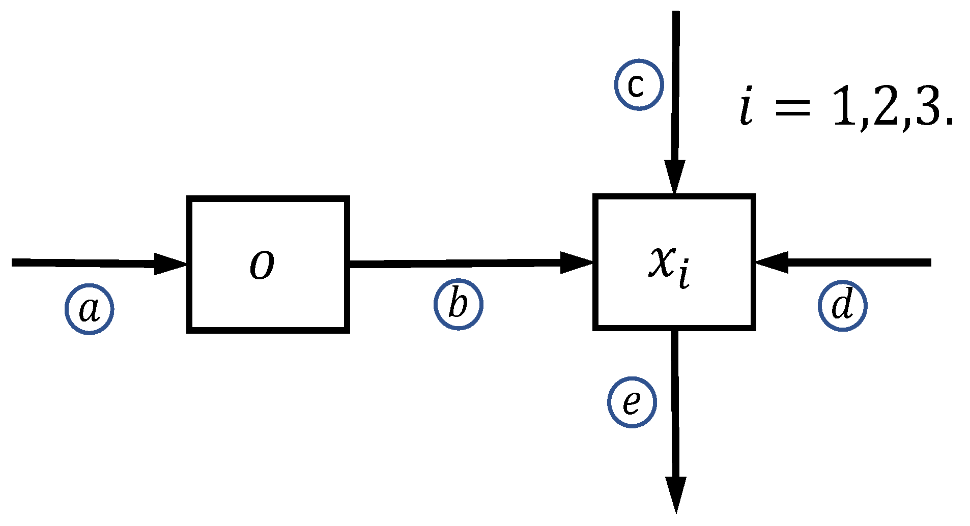
2. Model Conceptualization
Mathematical Formulation
3. Qualitative Analysis
3.1. Absence, Presence, and Coexistence of AMS
- (i)
- AM-free equilibrium: .
- (ii)
- Presence equilibrium: , , ,, and .
- (iii)
- Coexistence equilibrium: with
3.2. Stability Analysis
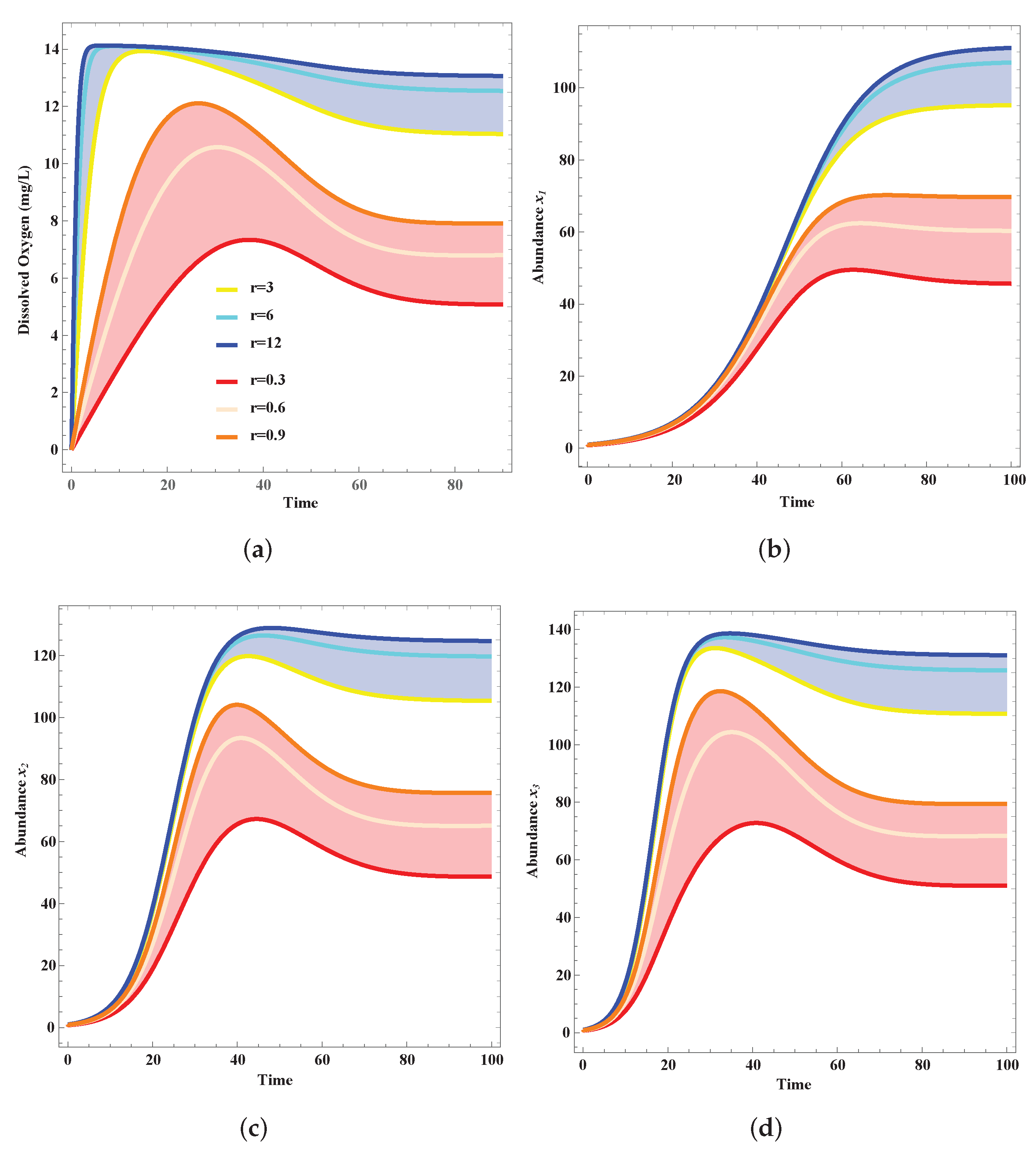
4. Results
Validation
5. Discussion
6. Conclusions
Author Contributions
Funding
Institutional Review Board Statement
Informed Consent Statement
Data Availability Statement
Acknowledgments
Conflicts of Interest
Appendix A. Mathematical Calculation
Appendix A.1. Jacobian Matrix
Appendix A.2. Coefficients
Appendix B. Parameters

References
- United Nations. Transforming our world: The 2030 agenda for sustainable development. In General Assembley 70 Session; United Nations: New York, NY, USA, 2015. [Google Scholar]
- Uddin, M.G.; Nash, S.; Olbert, A.I. A review of water quality index models and their use for assessing surface water quality. Ecol. Indic. 2021, 122, 3400–3411. [Google Scholar]
- Almeida, C.; González, S.O.; Mallea, M.; González, P. A recreational water quality index using chemical, physical and microbiological parameters. Environ. Sci. Pollut. Res. 2012, 19, 3400–3411. [Google Scholar] [CrossRef] [PubMed]
- Farhat, N.; Kim, L.H.; Vrouwenvelder, J.S. Online characterization of bacterial processes in drinking water systems. Npj Clean Water 2020, 3, 1–7. [Google Scholar] [CrossRef]
- Jørgensen, S.E.; Xu, F.L.; Salas, F.; Marques, J.C. Handbook of Ecological Indicators for Assessment of Ecosystem Health; CRC Press: Boca Raton, FL, USA, 2016; pp. 9–64. [Google Scholar]
- Hernández-Mira, F.A.; Rosas-Acevedo, J.L.; Reyes-Umaña, M.; Violante-González, J.; Sigarreta-Almira, J.M.; Vakhania, N. Multimetric Index to Evaluate Water Quality in Lagoons: A Biological and Geomorphological Approach. Sustainability 2021, 13, 4631. [Google Scholar] [CrossRef]
- Bain, M.B.; Stevenson, N.J. (Eds.) Aquatic Habitat Assessment: Commom Methods; Asian Fisheries Society: Bethesda, MD, USA, 1999; p. 186. ISBN 1-888569-18-2. [Google Scholar]
- Ejigu, M.T. Overview of water quality modeling. Cogent Eng. 2021, 8, 1891711. [Google Scholar] [CrossRef]
- Zhen-Gang, J. Hydrodynamics and Water Quality: Modeling Rivers, Lakes, and Estuaries; John Wiley & Sons: Hoboken, NJ, USA, 2017. [Google Scholar]
- Loucks, D.P.; Van Beek, E. Water Resource Systems Planning and Management: An Introduction to Methods, Models, and Applications; Springer: Cham, Switzerland, 2017. [Google Scholar]
- Gonenc, I.E.; Wolflin, J.P. (Eds.) Coastal Lagoons: Ecosystem Processes and Modeling for Sustainable Use and Development; CRC Press: Boca Raton, FL, USA, 2004. [Google Scholar]
- Jacoby, J.; Welch, E. Pollutant Effects in Freshwater: Applied Limnology, 3rd ed.; CRC Press: Boca Raton, FL, USA, 2004. [Google Scholar]
- Sánchez, E.; Colmenarejo, M.F.; Vicente, J.; Rubio, A.; García, M.G.; Travieso, L.; Borja, R. Use of the water quality index and dissolved oxygen deficit as simple indicators of watersheds pollution. Ecol. Indic. 2007, 7, 315–328. [Google Scholar] [CrossRef]
- Kannel, P.R.; Lee, S.; Lee, Y.S.; Kanel, S.R.; Khan, S.P. Application of water quality indices and dissolved oxygen as indicators for river water classification and urban impact assessment. Environ. Monit. Assess. 2007, 132, 93–110. [Google Scholar] [CrossRef]
- Best, M.A.; Wither, A.W.; Coates, S. Dissolved oxygen as a physico-chemical supporting element in the Water Framework Directive. Mar. Pollut. Bull. 2007, 55, 53–64. [Google Scholar] [CrossRef]
- Kannel, P.R.; Kanel, S.R.; Lee, S.; Lee, Y.S.; Gan, T.Y. A review of public domain water quality models for simulating dissolved oxygen in rivers and streams. Environ. Model. Assess. 2011, 16, 183–204. [Google Scholar] [CrossRef]
- Kaller, M.D.; Kelso, W.E. Association of macroinvertebrate assemblages with dissolved oxygen concentration and wood surface area in selected subtropical streams of the southeastern USA. Aquat. Ecol. 2007, 41, 95–110. [Google Scholar] [CrossRef]
- Wilhm, J.; McClintock, N. Dissolved oxygen concentration and diversity of benthic macroinvertebrates in an artificially destratified lake. Hydrobiologia 1978, 57, 163–166. [Google Scholar] [CrossRef]
- Wang, J.; Fu, Z.; Qiao, H.; Liu, F. Assessment of eutrophication and water quality in the estuarine area of Lake Wuli, Lake Taihu, China. Sci. Total Environ. 2019, 650, 1392–1402. [Google Scholar] [CrossRef] [PubMed]
- Meier, H.E.M.; Eilola, K.; Almroth-Rosell, E.; Schimanke, S.; Kniebusch, M.; Höglund, A.; Pemberton, P.; Liu, Y.; Väli, G.; Saraiva, S. Disentangling the impact of nutrient load and climate changes on Baltic Sea hypoxia and eutrophication since 1850. Clim. Dyn. 2019, 53, 1145–1166. [Google Scholar] [CrossRef]
- Zhang, J.; Wang, C.; Jiang, X.; Song, Z.; Xie, Z. Effects of human-induced eutrophication on macroinvertebrate spatiotemporal dynamics in Lake Dianchi, a large shallow plateau lake in China. Environ. Sci. Pollut. Res. 2020, 27, 1–15. [Google Scholar] [CrossRef]
- Bazzanti, M.; Mastrantuono, L.; Solimini, A.G. Selecting macroinvertebrate taxa and metrics to assess eutrophication in different depth zones of Mediterranean lakes. Fundam. Appl. Limnol. Hydrobiol. 2012, 180, 133–143. [Google Scholar] [CrossRef]
- Galic, N.; Hawkins, T.; Forbes, V.E. Adverse impacts of hypoxia on aquatic invertebrates: A meta-analysis. Sci. Total Environ. 2019, 652, 736–743. [Google Scholar] [CrossRef]
- Etemi, F.Z.; Bytyçi, P.; Ismaili, M.; Fetoshi, O.; Ymeri, P.; Shala–Abazi, A.; Muja-Bajraktari, N.; Czikkely, M. The use of macroinvertebrate based biotic indices and diversity indices to evaluate the water quality of Lepenci river basin in Kosovo. J. Environ. Sci. Heal. Part A 2020, 55, 748–758. [Google Scholar] [CrossRef]
- Slimani, N.; Sánchez-Fernández, D.; Guilbert, E.; Boumaiza, M.; Guareschi, S.; Thioulouse, J. Assessing potential surrogates of macroinvertebrate diversity in North-African Mediterranean aquatic ecosystems. Ecol. Indic. 2019, 101, 324–329. [Google Scholar] [CrossRef]
- Silva, D.R.O.; Herlihy, A.T.; Hughes, R.M.; Macedo, D.R.; Callisto, M. Assessing the extent and relative risk of aquatic stressors on stream macroinvertebrate assemblages in the neotropical savanna. Sci. Total Environ. 2018, 633, 179–188. [Google Scholar] [CrossRef]
- Croijmans, L.; de Jong, J.F.; Prins, H.H. Oxygen is a better predictor of macroinvertebrate richness than temperature—A systematic review. Environ. Res. Lett. 2020, 38, 1820–1832. [Google Scholar] [CrossRef]
- Su, P.; Wang, X.; Lin, Q.; Peng, J.; Song, J.; Fu, J.; Wang, S.; Cheng, D.; Bai, H.; Li, Q. Variability in macroinvertebrate community structure and its response to ecological factors of the Weihe River Basin, China. Ecol. Eng. 2019, 140, 105595. [Google Scholar] [CrossRef]
- Mezgebu, A.; Lakew, A.; Lemma, B. Water quality assessment using benthic macroinvertebrates as bioindicators in streams and rivers around Sebeta, Ethiopia. Afr. J. Aquat. Sci. 2019, 44, 361–367. [Google Scholar] [CrossRef]
- Liu, Z.; Fan, B.; Huang, Y.; Yu, P.; Li, Y.; Chen, M.; Cai, M.; Lv, W.; Jiang, Q.; Zhao, Y. Assessing the ecological health of the Chongming Dongtan Nature Reserve, China, using different benthic biotic indices. Mar. Pollut. Bull. 2018, 146, 76–84. [Google Scholar]
- Liu, Z.; Chen, M.; Li, Y.; Huang, Y.; Fan, B.; Lv, W.; Yu, P.; Wu, D.; Zhao, Y. Different effects of reclamation methods on macrobenthos community structure in the Yangtze Estuary, China. Mar. Pollut. Bull. 2018, 127, 429–436. [Google Scholar]
- Pineda-Pineda, J.J.; Rosas-Acevedo, J.L.; Sigarreta, J.M.; Hernández-Gómez, J.C.; Reyes-Umaña, M. Biotic Indices to Evaluate Water Quality: BMWP. Int. J. Environ. Ecol. Fam. Urban Stud. IJEEFUS 2018, 8, 23–36. [Google Scholar]
- Zhou, X.D.; Xu, M.Z.; Lei, F.K.; Zhang, J.H.; Wang, Z.Y.; Luo, Y.Y. Responses of Macroinvertebrate Assemblages to Flow in the Qinghai-Tibet Plateau: Establishment and Application of a Multi-metric Habitat Suitability Model. Water Resour. Res. 2022, 58, e2021WR030909. [Google Scholar] [CrossRef]
- Pineda-Pineda, J.J.; Martínez-Martínez, C.T.; Méndez-Bermúdez, J.A.; Muñoz-Rojas, J.; Sigarreta, J.M. Application of Bipartite Networks to the Study of Water Quality. Sustainability 2020, 12, 5143. [Google Scholar] [CrossRef]
- Schleiter, I.M.; Borchardt, D.; Wagner, R.; Dapper, T.; Schmidt, K.D.; Schmidt, H.H.; Werner, H. Modelling water quality, bioindication and population dynamics in lotic ecosystems using neural networks. Ecol. Model. 1999, 120, 271–286. [Google Scholar] [CrossRef]
- Maier, H.R.; Dandy, G.C. The use of artificial neural networks for the prediction of water quality parameters. Water Resour. Res. 1996, 32, 1013–1022. [Google Scholar] [CrossRef]
- Villamarín, C.; Rieradevall, M.; Paul, M.J.; Barbour, M.T.; Prat, N. A tool to assess the ecological condition of tropical high Andean streams in Ecuador and Peru: The IMEERA index. Ecol. Indic. 2013, 29, 79–92. [Google Scholar] [CrossRef]
- Karaouzas, I.; Smeti, E.; Kalogianni, E.; Skoulikidis, N.T. Ecological status monitoring and assessment in Greek rivers: Do macroinvertebrate and diatom indices indicate same responses to anthropogenic pressures? Ecol. Indic. 2019, 101, 126–132. [Google Scholar] [CrossRef]
- El Sayed, S.M.; Hegab, M.H.; Mola, H.R.; Ahmed, N.M.; Goher, M.E. An integrated water quality assessment of Damietta and Rosetta branches (Nile River, Egypt) using chemical and biological indices. Environ. Monit. Assess. 2020, 192, 1–16. [Google Scholar] [CrossRef] [PubMed]
- Streeter, H.W.; Phelps, E.B. A Study of the Pollution and Natural Purification of the Ohio River; Public Health Bulletin No 146; Public Health Service: Washington, DC, USA, 1925.
- Wang, Q.; Li, S.; Jia, P.; Qi, C.; Ding, F. A review of surface water quality models. Sci. World J. 2013. [Google Scholar] [CrossRef]
- da Silva Burigato Costa, C.M.; Leite, I.R.; Almeida, A.K.; de Almeida, I.K. Choosing an appropriate water quality model—A review. Environ. Monit. Assess. 2021, 193, 1–15. [Google Scholar] [CrossRef]
- Park, R.A.; Clough, J.S.; Wellman, M.C. AQUATOX: Modeling environmental fate and ecological effects in aquatic ecosystems. Ecol. Model. 2008, 213, 1–15. [Google Scholar] [CrossRef]
- West Virginia Department of Environmental Protection. Available online: https://dep.wv.gov/WWE/getinvolved/sos/Documents/Benthic/VisualMacroGuide.pdf (accessed on 1 September 2022).
- Researchgate. Available online: https://www.researchgate.net/profile/Pablo-Gutierrez-Fonseca/publication/295854904_Guia_fotografica_de_familias_de_macroinvertebrados_acuaticos_de_Puerto_Rico/links/56ce23e508aeb52500c36b4f/Guia-fotografica-de-familias-de-macroinvertebrados-acuaticos-de-Puerto-Rico.pdf (accessed on 1 September 2022).
- Everaert, G.; De Neve, J.; Boets, P.; Dominguez-Granda, L.; Mereta, S.T.; Ambelu, A.; Hoang, T.H.; Goethals, P.L.M.; Thas, O. Comparison of the abiotic preferences of macroinvertebrates in tropical river basins. PLoS ONE 2014, 9, e108898. [Google Scholar] [CrossRef] [PubMed]
- Weiwei, L.; Youhui, H.; Zhiquan, L.; Yang, Y.; Bin, F.; Yunlong, Z. Application of macrobenthic diversity to estimate ecological health of artificial oyster reef in Yangtze Estuary, China. Mar. Pollut. Bull. 2016, 103, 137–143. [Google Scholar]
- Weiwei, L.; Zhiquan, L.; Yang, Y.; Youhui, H.; Bin, F.; Qichen, J.; Yunlong, Z. Loss and self-restoration of macrobenthic diversity in reclamation habitats of estuarine islands in Yangtze Estuary, China. Mar. Pollut. Bull. 2016, 103, 128–136. [Google Scholar]
- Pearl, R.; Reed, L.J. On the rate of growth of the population of the United States since 1790 and its mathematical representation. Proc. Natl. Acad. Sci. USA 1920, 6, 275. [Google Scholar] [CrossRef]
- Hutchinson, G.E. An Introduction to Population Ecology; Yale University Press: New Haven, CT, USA, 1978. [Google Scholar]
- Chapman, E.J.; Byron, C.J. The flexible application of carrying capacity in ecology. Glob. Ecol. Conserv. 2018, 13, e00365. [Google Scholar]
- Gunderson, L.H. Ecological resilience-in theory and application. Annu. Rev. Ecol. Syst. 2000, 31, 425–439. [Google Scholar] [CrossRef]
- Rosas-Acevedo, J.L.; Ávila-Pérez, H.; Sánchez-Infante, A.; Rosas-Acevedo, Y.; García-Ibañez, S.; Sampedro-Rosas, L.; Granados-Ramírez, J.G.; Juárez-López, A.L. índice BMWP, FBI y EPT para determinar la calidad del agua en la laguna de Coyuca de Benítez, Guerrero, México. Rev. Iberoam. Cienc. 2014, 1, 81–88. [Google Scholar]
- Rosińska, J.; Kozak, A.; Dondajewska, R.; Kowalczewska-Madura, K.; Gołdyn, R. Water quality response to sustainable restoration measures–Case study of urban Swarzędzkie Lake. Ecol. Indic. 2018, 84, 437–449. [Google Scholar] [CrossRef]
- Gołdyn, R.; Podsiadłowski, S.; Dondajewska, R.; Kozak, A. The sustainable restoration of lakes—Towards the challenges of the Water Framework Directive. Ecohydrol. Hydrobiol. 2014, 14, 68–74. [Google Scholar] [CrossRef]
- Kail, J.; Brabec, K.; Poppe, M.; Januschke, K. The effect of river restoration on fish, macroinvertebrates and aquatic macrophytes: A meta-analysis. Ecol. Indic. 2015, 58, 311–321. [Google Scholar] [CrossRef]


| Parameter | Description | Value | Reference |
|---|---|---|---|
| r | oxygenation/aeration rate | 0–14.5 mgL−1 | Galic et al. [23] |
| m | oxygen saturation constant a | 0 < m ≤ 14.5 mgL−1 | |
| βi | average respiration rate of AMs a | 0–0.918 | Galic et al. [23] |
| ri | average reproduction rate of AMs a | 0–1.02 | Galic et al. [23] |
| ki | average carrying capacity of AMs | varies | |
| γi | average DO utilization rate | varies |
| Relation | Meaning | Water Quality |
|---|---|---|
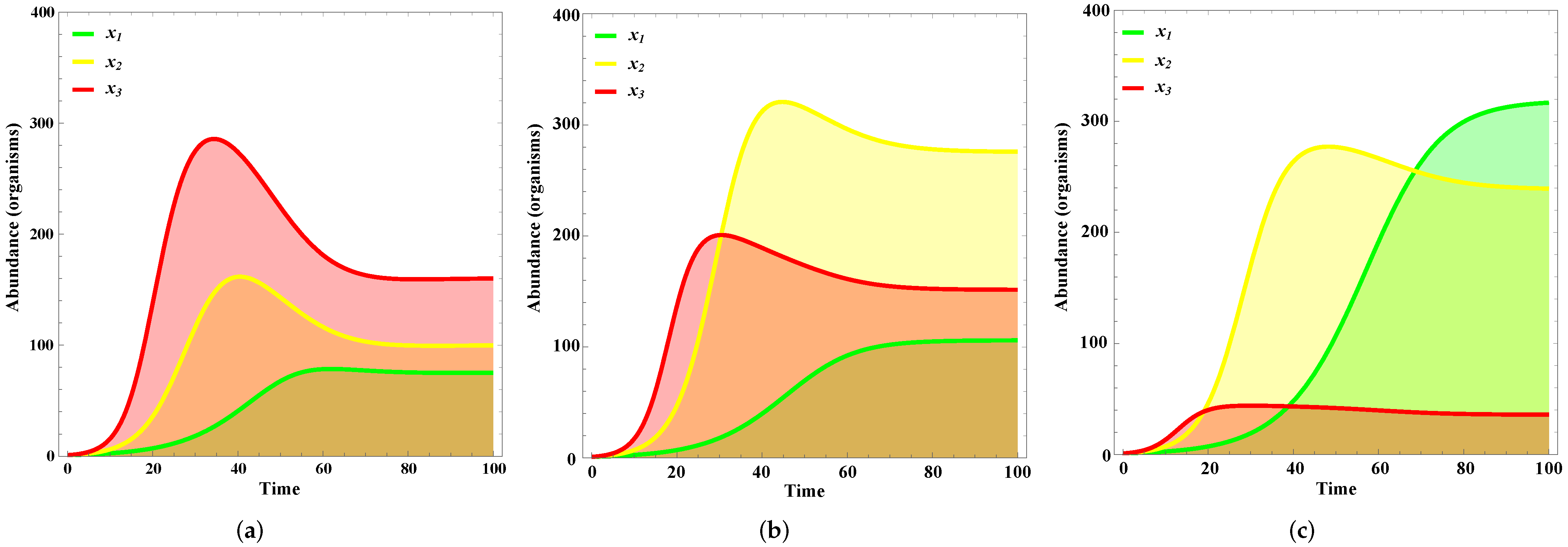
| x3 < x2 < x1 | Low pollution with a tendency to increase | good |
| x3 < x1 < x2 | Regular pollution with a tendency to decrease | moderate |
| x2 < x3 < x1 | Low pollution with a tendency to increase | good |
| x2 < x1 < x3 | High pollution with a tendency to decrease | poor |
| x1 < x3 < x2 | Regular pollution with a tendency to increase | moderate |
| x1 < x2 < x3 | High pollution with a tendency to decrease | poor |
Publisher’s Note: MDPI stays neutral with regard to jurisdictional claims in published maps and institutional affiliations. |
© 2022 by the authors. Licensee MDPI, Basel, Switzerland. This article is an open access article distributed under the terms and conditions of the Creative Commons Attribution (CC BY) license (https://creativecommons.org/licenses/by/4.0/).
Share and Cite
Pineda-Pineda, J.J.; Muñoz-Rojas, J.; Morales-García, Y.E.; Hernández-Gómez, J.C.; Sigarreta, J.M. Biomathematical Model for Water Quality Assessment: Macroinvertebrate Population Dynamics and Dissolved Oxygen. Water 2022, 14, 2902. https://doi.org/10.3390/w14182902
Pineda-Pineda JJ, Muñoz-Rojas J, Morales-García YE, Hernández-Gómez JC, Sigarreta JM. Biomathematical Model for Water Quality Assessment: Macroinvertebrate Population Dynamics and Dissolved Oxygen. Water. 2022; 14(18):2902. https://doi.org/10.3390/w14182902
Chicago/Turabian StylePineda-Pineda, Jair J., Jesús Muñoz-Rojas, Y. Elizabeth Morales-García, Juan C. Hernández-Gómez, and José M. Sigarreta. 2022. "Biomathematical Model for Water Quality Assessment: Macroinvertebrate Population Dynamics and Dissolved Oxygen" Water 14, no. 18: 2902. https://doi.org/10.3390/w14182902