
Economic Analysis of Flood Risk Applied to the Rehabilitation of Drainage Networks
by
 , , and
Leonardo Bayas-Jiménez
1,2,* ,
,
F. Javier Martínez-Solano
1 ,
,
Pedro L. Iglesias-Rey
1 and
Fulvio Boano
2 1
Department of Hydraulic Engineering and Environment, Universitat Politècnica de València, Camino de Vera s/n, 46022 Valencia, Spain
2
Department of Environment, Land, and Infrastructure Engineering, Politecnico di Torino, Corso Duca degli Abruzzi, 24, 10129 Turin, Italy
*
Author to whom correspondence should be addressed.
Water 2022, 14(18), 2901; https://doi.org/10.3390/w14182901
Submission received: 16 August 2022
/
Revised: 9 September 2022
/
Accepted: 14 September 2022
/
Published: 16 September 2022
(This article belongs to the Special Issue Flooding in Urban Areas: Risks and Responses)
Abstract
:Over time, cities have grown, developing various activities and accumulating important economic assets. Floods are a problem that worry city administrators who seek to make cities more resilient and safer. This increase in flood events is due to different causes: poor planning, population increase, aging of networks, etc. However, the two main causes for the increase in urban flooding are the increment in frequency of extreme rainfall, generated mainly by climate change, and the increase in urbanized areas in cities, which reduce green areas, decreasing the percentage of water that seeps naturally into the soil. As a contribution to solve these problems, the work presented shows a method to rehabilitate drainage networks that contemplates implementing different actions in the network: renovation of pipes, construction of storm tanks and installation of hydraulic controls. This work focuses on evaluating the flood risk in economic terms. To achieve this, the expected annual damage from floods and the annual investments in infrastructure to control floods are estimated. These two terms are used to form an objective function to be minimized. To evaluate this objective function, an optimization model is presented that incorporates a genetic algorithm to find the best solutions to the problem; the hydraulic analysis of the network is performed with the SWMM model. This work also presents a strategy to reduce computation times by reducing the search space focused mainly on large networks. This is intended to show a complete and robust methodology that can be used by managers and administrators of drainage networks in cities.
1. Introduction
Urban drainage infrastructure is built at high cost and represents an important asset of cities that is expected to have a long service life. However, the occurrence of floods in cities is becoming more and more evident, generating concern for engineers and managers of city drainage systems. The increase in the frequency of extreme rainfall events is notorious; many studies have delved into the causes of this increase [1,2] and are able to conclude that it is due to an increase in rainfall intensity, mainly due to climate change. In addition to this fact, the growth of cities has decreased the number of green spaces, replacing them with impervious surfaces that increase runoff, aggravating the flooding problem [3,4,5,6]. These conditions have generated frequent floods that generate heavy losses in cities [7,8,9]. O’Donnell and Thorne [10] mention that, by 2050, 68% of the world’s population will live in urban areas, so taking measures against flood risk is of primary importance. Rehabilitating drainage networks is a topic of growing interest for researchers; the use of storm tanks (STs) to mitigate runoff peaks in extreme rainfall events has proven to be an efficient alternative [11,12]. For this reason, their use has been considered in the present work in conjunction with the classical approach of renovating pipes. Furthermore, the inclusion of hydraulic controls (CHs) to rehabilitate networks is considered. For the optimization process of drainage networks, researchers have used different methodologies, highlighting the use of evolutionary algorithms that give good results in water resource research [13]; of these, genetic algorithms show great performance in the search for the best solutions due to their adaptation to complex landscapes [14,15]. The pseudo-genetic algorithm (PGA) used in this work has shown robustness and efficiency in finding solutions, and is easier to implement in optimization models [16]. However, computation times can be very long due to the large search space (SS) that the algorithm must explore. To improve the performance of the algorithms, some strategy must be implemented to optimize the search. One way to do this is to decrease the SS by identifying the best regions containing the best solutions and discarding the less attractive ones. Different works have been carried out with this method [17,18], demonstrating that these strategies can improve the efficiency of optimization models. In this way, in a previously performed work, Bayas-Jiménez et al. [14] present a methodology for search space reduction (SSR) focusing on the recursive reduction of decision variables (DVs) with the use of reduced option lists to identify the best search regions. In this work, an SSR method based on the method of Bayas-Jiménez et al. [14] is used, focusing on reducing the SS in large networks to improve the efficiency of the rehabilitation methodology.
On the other hand, in the work carried out by Bayas-Jiménez et al. [12], the authors present a methodology to rehabilitate drainage networks and improve the efficiency of the optimization model. However, one of the drawbacks of this methodology is the joint evaluation of total investment costs and damage costs for a single rainfall. Although it is a valid methodology, which shows in monetary amounts the advantages of rehabilitating the network using the highest intensity rainfall that the drainage system will face, it does not show us the cost of flood damages with rainfall lower than the return period (T) used. These lower intensity rains can present significant damages in the study area, as rightly mentioned by Freni et al. [19]. For this reason, and with the objective of improving the methodology, this work focuses on determining the annual damage cost that can be caused by floods and annualizing the cost of the required investment. To determine the annual cost of flood damage, we have reviewed the work done by Zhou et al. [20] and Olsen et al. [21], who present models to identify low-cost adaptation measures that mitigate events with high annual risk. In this way, the cost of flood risk is calculated by integrating the area under the curve generated by flood damage in the return periods considered. Finally, a solution is obtained that integrates the annual cost of the flood risk and the annual investment that would be required to face it. This work also emphasizes the need to implement a SSR strategy in the methodology so that a method that significantly reduces calculation times is used. It is important to mention that the optimization model uses the storm water management model (SWMM) to analyze the network; this model completely solves the Saint-Venant equations. For the hydraulic analysis with SWMM, the dynamic wave model is used with the Darcy–Weisbach as the main force equation. The methodology also assumes that flooding occurs by water stagnation, i.e., that the total volume of runoff enters the manholes through the gutters of the system. However, this methodology has certain limitations that must be considered:
- The hydrologic study and the runoff model are beyond the scope of this work;
- No changes in the network topology are considered. The actions allowed to improve the network are the replacement of pipes, the installation of storm tanks and the inclusion of hydraulic control elements in the network;
- The networks in which this methodology can be applied must be gravity-fed. Networks with pumping systems are not considered in this study;
- The hydraulic model is considered as a datum; its parameters and initial conditions are not questioned.
With this work, the authors intend to show a robust methodology that encompasses solutions to the difficulties that may arise in the rehabilitation of drainage networks, providing different alternatives to reduce calculation times and ensure that the optimization criterion satisfies the expectations of network managers.
2. Materials and Methods
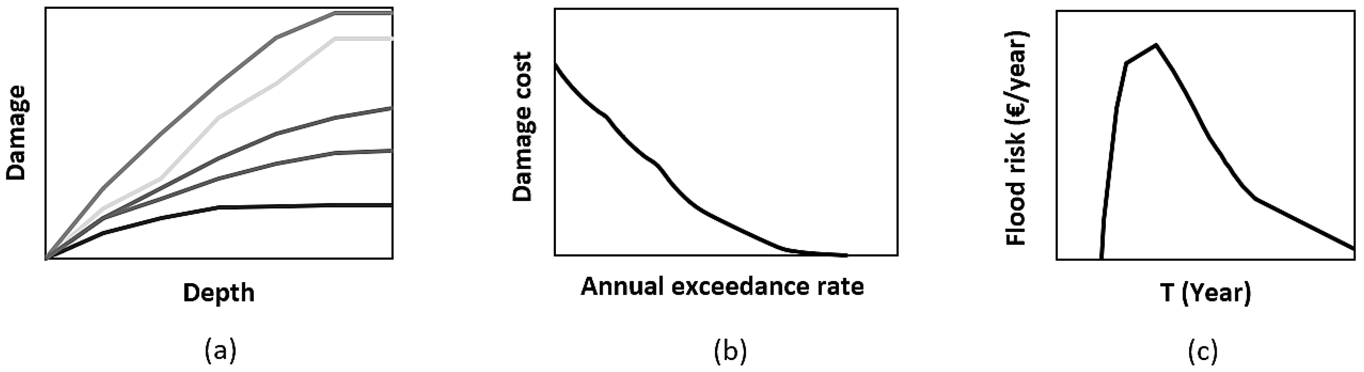
The methodology considered carrying out different actions in the drainage network to reduce the risk of flooding in the studied area. These actions were: the replacement of pipes by others of larger diameter; the construction of small STs to replace the existing wells; and the installation of hydraulic control elements to slow down the flow of water in the network. To determine where these elements would be implemented and what characteristics they would have, an optimization model was used. The model used a PGA as an optimization engine [22]. The hydraulic analysis of the model was performed with the SWMM model [23] connected to the PGA through a toolkit developed by Martínez-Solano et al. [24]. This way of rehabilitating drainage networks was presented in a previous work by Bayas-Jiménez et al. [12], demonstrating its advantages by decreasing the cost of flood damage. However, this methodology analyzes flood costs for a single design rainfall. Although it is true that this rainfall event is the one that is going to demand the most from the system, the methodology does not consider other rain events of lesser intensity that may occur with greater probability in the design period and could generate floods. To solve this problem, this work modified the way of quantifying flood damage by focusing on the analysis of flood risk. Land use and rainfall magnitude are the most important characteristics in flood risk analysis. The study of these characteristics in urban areas and the relationship between them has resulted in the so-called damage–depth curves (Figure 1a) that relate the damage in monetary units or percentage and the depth of flooding. These curves are intended to represent the vulnerability of cities to flood risk [25].
One tool used as an indicator of vulnerability is the expected annual damage (EAD) [26]. This method estimates the average flood damage calculated for a series of events. The method considers that if the annual exceedance rate can be expressed as the inverse of T and the damages in monetary units, different values of flood damages can be calculated for different return periods, thus defining a curve (Figure 1b). In this way, the average annual flood risk can be calculated by integrating the area under this curve [27]. In the work carried out by Olsen et al. [21], the authors compared different methods for estimating flood risk in urban drainage systems. In addition to these comparisons, the authors emphasize that, as return periods increase, flood damage costs also increase, but the annual exceedance rate also decreases, as can be seen in the flood risk density curve (Figure 1c).
It was necessary to integrate this way of evaluating flooding into the methodology by relating it to the annualized infrastructure investment costs. With this objective in mind, an optimization model was developed that could find the best solution to the raised issue.
2.1. Optimization Model
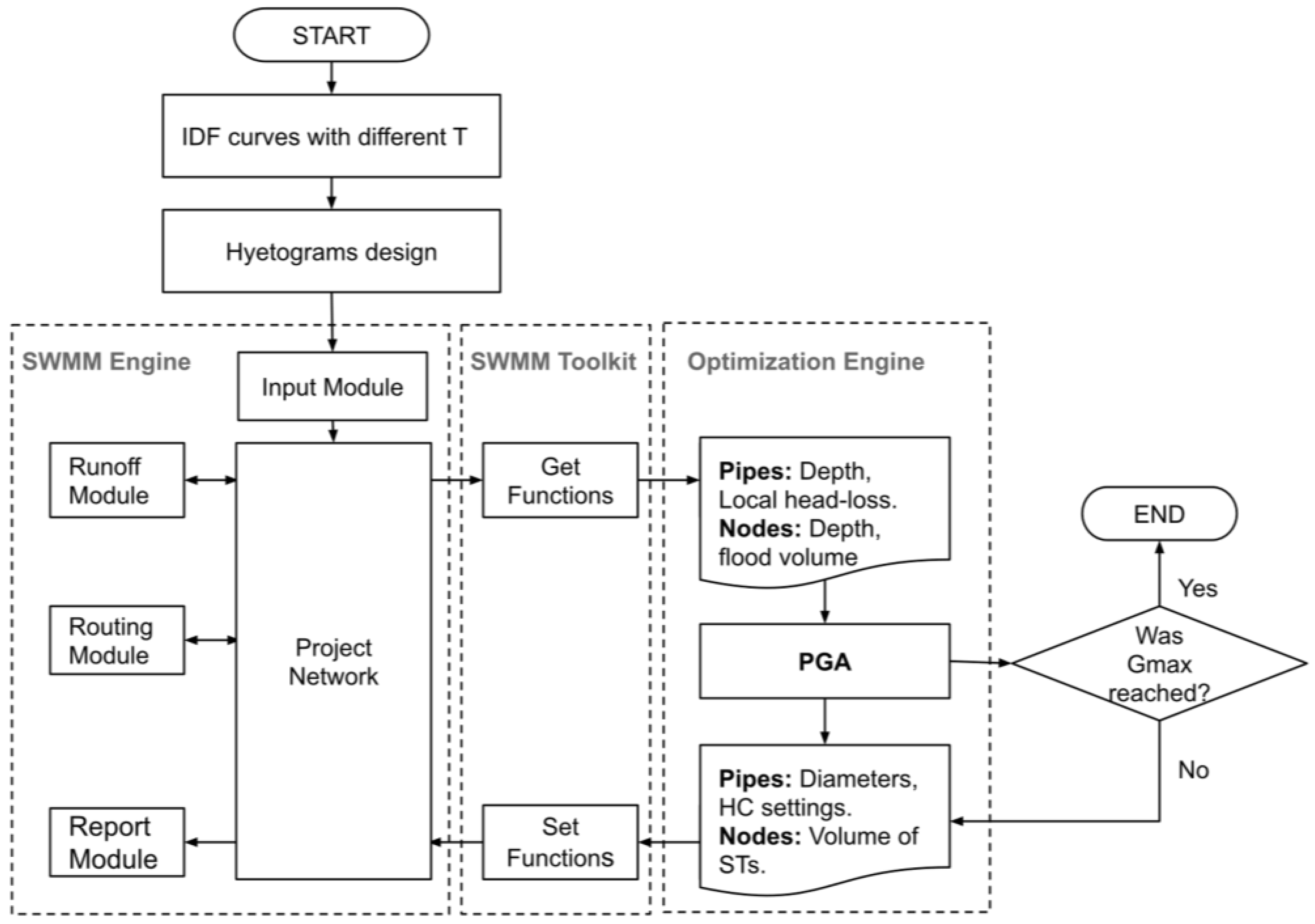
The optimization model used a PGA as a search engine; this type of algorithm, unlike traditional genetic algorithms, uses an integer encoding. The PGA was connected to the SWMM model through a toolkit to perform a series of simulations to find an optimal solution to the problem. To achieve this, the PGA evaluated an objective function composed of two types of cost functions: the annualized costs of infrastructure investment and the costs of the annual cost of flood risk. This implied that design rainfalls must be defined in advance for different return periods. The rainfall was constructed by means of a design hyetograph obtained through the analysis of intensity–duration–frequency (IDF) curves. These rainfalls were introduced into the network to be analyzed by the model. Figure 2 summarizes the operation of the optimization model. The optimization process was iterative and required establishing an end point for a process called the convergence criterion (Gmax). This criterion considers that when the value of the objective function does not change during a certain number of generations, the objective function has reached its minimum and the process ends. Gmax is explained in depth in the work presented by Bayas-Jiménez et al. [14].
2.1.1. Decision Variables
Since this methodology used a PGA for optimization, the DVs were required to take values from lists of options with discrete values. In order to perform the network optimization, it was necessary to clearly define the DVs used in this methodology. The methodology considered three types of DVs. The first type of DVs considered was pipe diameter. In the optimization process, the pipes selected to be optimized could take values from the existing diameter range NDmax. The previously defined list of options for optimization, called ΔND, was composed of a small number of diameters immediately larger than the analyzed pipe diameter. This decision was taken because pipes in the optimization process would only take values larger than the current diameter, so defining lists using the whole range of pipes would only increase the computational effort unnecessarily; with this action, the size of the problem was considerably decreased.
The second type of DVs considered was the storage capacity of the STs. This work considered the depth of the STs to be the same as the existing manholes, so the cross section of the STs was defined as a DV. In the optimization process, the nodes selected to be optimized ns could take values from a previously defined list of options. As shown in Section 2.2, the methodology was composed of two stages. In the first stage, a coarse option list NS0 was used and for the second stage, a refined option list NSmax was used. Finally, the third type of DVs considered the head-loss values that the hydraulic control element installed in the pipes could generate. In the optimization process, the selected pipes vs could have hydraulic controls with a degree of openness from a previously defined option list Nθ.
2.1.2. Cost Functions
In order to define the objective function that the optimization model would evaluate, the first step was to establish the cost functions of the investments in infrastructure and the cost of the flood risk.
The first infrastructure investment cost function was the replacement of pipes. To determine this cost, the cost of acquisition and installation of pipes was analyzed for different diameters.
According to the values obtained, an equation was defined that fits a second-degree polygonal curve and is presented as Equation (1).
In the equation, Cp(Di) represents the pipe replacement cost in euros, Di is the pipe diameter and Li represents the pipe length in meters. The coefficients α, β and γ are adjustment coefficients corresponding to each project.
The second infrastructure investment cost function was the cost of STs. To define this function, the cost of building tanks of different sizes was analyzed. With these data, a cost function composed of two terms was determined and is shown in Equation (2).
where CT(Vi) represents the cost in euros of the construction of a storm tank. Cmin represents the minimum cost of building a storm tank. Vi is the flood volume that the tank must store in cubic meters. Cvar and ω are coefficients corresponding to the analyzed project. The third structural investment cost function determined for this work was the cost of hydraulic control. To define this function, the cost of purchasing and installing valves of different diameters was analyzed. This analysis determined a second-degree polynomial function, shown in Equation (3).
where Cv(Di) is the cost of the hydraulic control in euros, Di is the diameter of the pipe where the hydraulic control would be installed, in meters, and σ, μ and φ are adjustment coefficients of the analyzed project.
On the other hand, to account for the reduction in investment in infrastructure, an annual amortization factor Λ was required that affects each cost function. In this work, the expression shown by Steiner (2007) was used and is shown in Equation (4).
In the equation, r is the annual interest and t is the time in years in which the investment is expected to be recovered.
Determining flood costs is a complicated task, since there are many aspects to be considered and they are commonly divided into two categories: intangible damages and tangible damages. Tangible damages are those that can be expressed in monetary terms and are those that have been widely used in the analysis of flood damages in urban areas. One of the most widely used techniques for flood damage analysis is to use flood depth or flood level as a reference. The analysis based on the flood level allows the reduction of flooding and the cost of flooding, depending on the flood zone. An expression that calculates the cost of flood damage as a function of flood depth and land use is the damage–depth curve; thus, an expression that allows this calculation is presented in Equation (5).
In Equation (7), Cy(yi) represents the damage cost in euros and ymax is the maximum depth at which the flooding reaches the maximum damage in meters. Cmax is the maximum flood damage cost obtained when ymax is reached, Ai is the flood area of the analyzed subcatchment in square meters, yi is the reached depth of the analyzed node in meters and λ and υ are adjustment coefficients based on historical flood damage data.
Once the cost of flooding had been defined, to proceed in analyzing the flood risk, we started from the work presented by Arnbjerg-Nielsen and Fleischer [28], who proposed a way of estimating the annual damage by relating the cost of flood damage from rainfall of various return periods. The authors conclude that the annual damage can be obtained by integrating the area under the curve obtained from plotting the flood cost (Cy(Di)) as a function of its annual exceedance rate (p). In a more recent work, Olsen et al. [21] mention that a good approximation of the curve can be obtained with a log-linear relationship and that, when integrated, it can show the average annual cost of flood risk; Figure 3 shows this relationship.
The equation of the line obtained from this assumption takes the form of the expression shown in Equation (6), where a and b are the coefficients of the line.
To integrate Equation (6), the lower limit 0 was defined as representing the annual exceedance rate associated with an event, with an infinite value of T and p0 representing the annual exceedance rate for which flood damage begins to occur (Equation (7)). Equation (8) shows how to calculate the annual flood risk cost CF(p).
Finally, with all the costs defined, an objective function that the optimization model sought to minimize was proposed. Equation (9) shows the objective function.
2.2. Optimization Process
2.2.1. Search Space Reduction
The SS basically depends on two elements: the DVs and each of the values that these DVs can adopt. When using a PGA, it is mandatory to discretize the SS, i.e., the values that the DVs take must be chosen from a list of options composed of a finite number of values. In this way, the discretization must be carried out carefully. Bayas-Jiménez et al. [14] mentions that an excessive refinement of the SS would greatly increase the SS and would require a very large computational effort. However, if the discretization is coarse, the precision of the results is diminished. The authors also propose an expression to determine the size of the SS, presented in Equation (10).
where ΔND, NS and Nθ represent the options lists used for pipes, STs and HCs, respectively. Some work has been done with the objective of identifying the areas of the SS that contain the best solutions. The works focus on two ways to reduce the SS, some focusing on the change of the search region [18,29], and others focusing on changing the algorithm’s operation [30,31]. In this work, a method based on the change of the search region was used. In summary, the method reduced the SS by identifying and eliminating decision variables that were not part of the optimal search region.
Due to the fact that, in networks of large sizes, the computational effort can be important and consume significant computational time, the SSR method called clustering is presented based on the work presented by Bayas et al. [14]. This method allows a reduction in the search region based on the identification of the most promising regions in a parallel way in the drainage network.
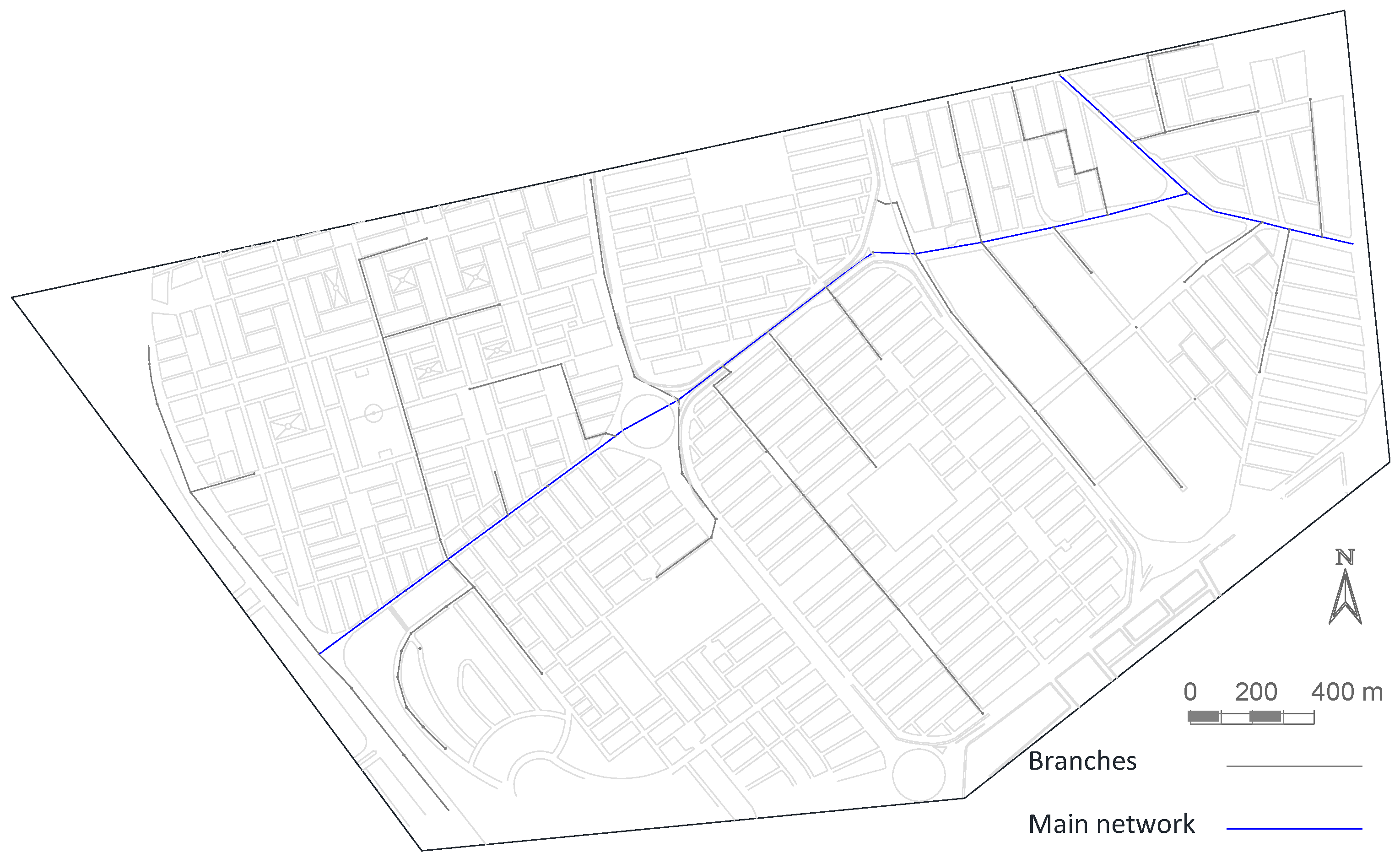
Drainage networks are generally made up of branches that collect rainwater from specific areas previously defined in the design stage of the drainage network. The water carried by these branches is discharged into a main network that collects the water from all the branches and transports it to treatment plants. Figure 4 shows an example of this network configuration.
It can be said that the network can be viewed as a set of sectors. If these sectors can be identified, a particular analysis of them can be performed to reduce the number of DVs within the sector and, consequently, reduce the overall SS. To perform the network analysis, it was necessary to make changes in the optimization model to analyze each sector that made up the drainage network in parallel. Once the sectors were fully defined, a series of evaluations were performed independently and in parallel with coarse option lists NS0 for nodes. In the case of pipes, and in order to optimize the process, a ΔND list of diameters immediately larger than analyzed pipe was used.
The results obtained were analyzed and the selection criterion proposed by Bayas-Jiménez et al. [14] was applied. In the same way, a lax Gmax was used because the objective was to eliminate DVs quickly and not to optimize the network. This process is applied iteratively until DVs could not be reduced further. Once the best regions of each sector were defined, a new search was made in the complete network, with the ns and ms selected in the sectors to finally delimit the optimal search region. It should be noted that the clustering method required significant computational use, so the method required the use of a cluster server to take advantage of its characteristics. Thus, despite the fact that several analyses were carried out, when they were carried out at the same time, and when working with sectors with fewer DVs, results were achieved in less time.
2.2.2. Final Optimization
Finally, after applying the SSR method, a final optimization was performed to find the solution closest to the optimum. Hydraulic controls were included in this stage; since their installation was linked to the installation of an ST, they were not considered in the SSR process. Likewise, at this stage, each of the DVs that made up the final search region were required to be explored in depth. Consequently, a refined (or full option) list NSmax was used for STs. In the case of pipes, the same ΔND range of diameters immediately larger than the analyzed pipes was used. Finally, for the HCs, a list of options Nθ was used that defined the degrees of opening that the element could adopt. At this stage, a more demanding Gmax was also used to find the closest solution to the optimum. This is the process that was followed to obtain the solution to the problem analyzed with the proposed methodology.
2.3. Case Studies
2.3.1. Balloon Network
The Balloon network is part of a drainage network located in a city in northern Italy. The network covers an area of 40.88 hectares. With a length of 1.85 km, the network is in a flat area whose highest point has an elevation of 229 m above sea level and the lowest point of 221 m above sea level. The network is made up of 71 pipes and 70 nodes. A total of 75 drainage sub-basins discharge their waters into the network. Figure 5 shows a schematic of the Balloon network. The entire network is gravity-fed. One problem with the network is the low slope of some of the pipes due to the topographical conditions of the area. To improve network circulation, the network has been designed with deep manholes reaching depths of more than 10 m. Despite this, the network has frequent flooding problems and needs to be rehabilitated. With the methodology and parameters used in this work, the network would present costs associated with the risk of flooding of 733,282 euros per year.
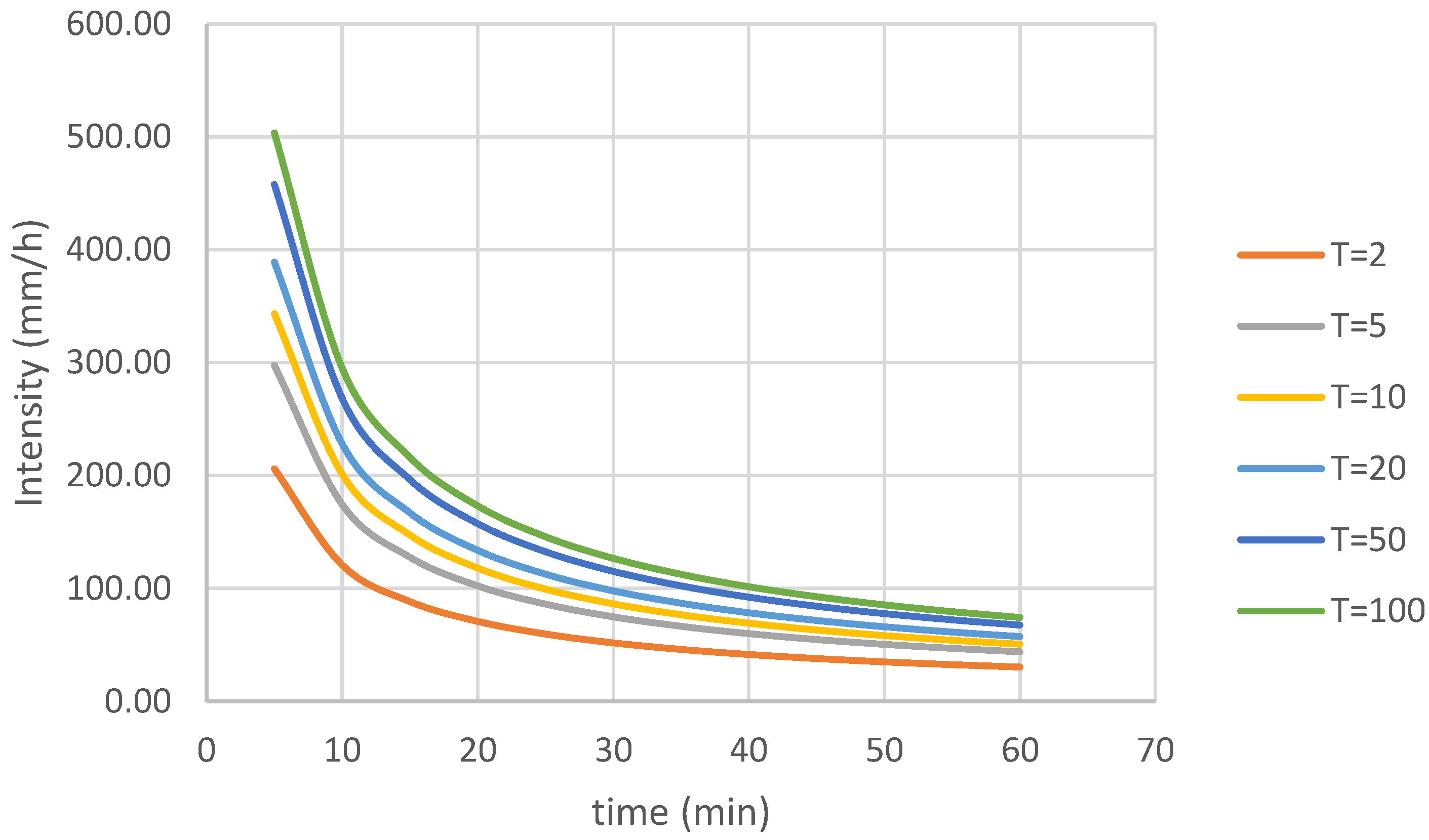
For the analysis of the network, design rainfalls were constructed using the alternating block method for return periods of 2, 5, 10, 20, 50 and 100 years. The IDF curves for the return periods studied are shown in Figure 6. Similarly, the land uses and the percentage they occupy in the study area are shown in Table S3 of the supplementary material of this work.
2.3.2. ES-N Network
The ES-N network is located in the city of Bogotá, Colombia. The network is made up of 385 nodes, 385 conduits and 385 hydrological sub-basins covering an area of 123.24 ha (Figure 7). The network has a total length of 20.11 km. The topography of the area is relatively flat with an average slope of 0.39%. However, the network has been designed to operate entirely by gravity, with pipes located more than 4 m deep. The network is made up of circular pipes with diameters ranging from 0.20 m to 1.40 m. Considering the methodology presented in this work, the network would present costs associated with the risk of flooding of 118,955 euros per year.
For the case study, two rainfalls were defined, designed with two return periods of 50 and 100 years and calculated by the method of alternating blocks with 10-min intervals. Rainfall was calculated from previously defined IDF curves. The curves obtained are shown in Figure 8. On the other hand, for the network study, the percentage of different land uses in the study area were established. Table S6 of the supplementary material shows these land uses.
2.3.3. Investment Costs
To define the coefficients of the cost function, a study was conducted on the prices of pipes of different commercially available diameters, as well as the cost of their installation. Figure 9 shows the cost curve of the pipes of the existing diameters per linear meter and the adjustment of the curve produced by these values. The same graph shows the equation with the coefficients obtained.
To determine the cost function of the STs, a study was conducted on the cost of the construction of these tanks of different sizes, including the excavation and removal of the excavated material. According to these costs, the curve shown in Figure 9 was determined, as well as the expression with the coefficients obtained.
Similarly, a study was conducted on the cost of gate valves, accessories and complementary installations necessary for the installation of HCs in pipelines. Figure 9 shows the costs of different HCs with commercially available diameters. The equation with the coefficients obtained is also shown.
As for the annual amortization factor, considering the design period and the type of construction, an interest rate of 3% and an investment return time of 20 years was fixed.
2.3.4. Flood Costs
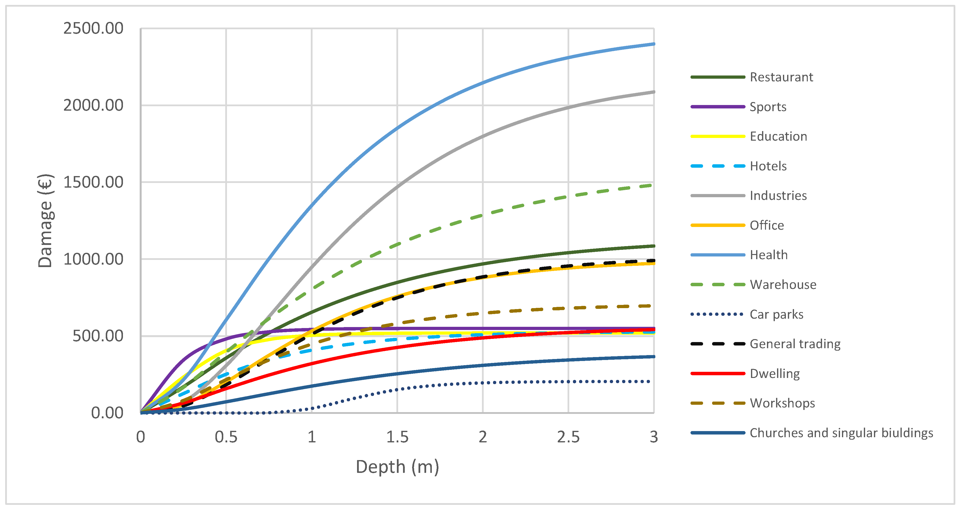
For the study of flood costs, the damage–depth curves presented by Martínez-Gomariz et al. [32] were analyzed. The authors present a series of curves for different types of buildings. Taking these curves as a reference, Equation (7) was used to determine the flood damage cost for different land uses. The expression adjusted quite well to the values that the authors present. Table S7 of the Supplementary Material shows the goodness of fit. Figure 10 shows the damage–depth curves obtained. Thus, all the cost functions required for the study of risk in economic terms for the developed model were defined. The coefficients used to define the curves for the different land uses analyzed are shown in Table S8 of the Supplementary Material.
3. Results
3.1. Balloon Network
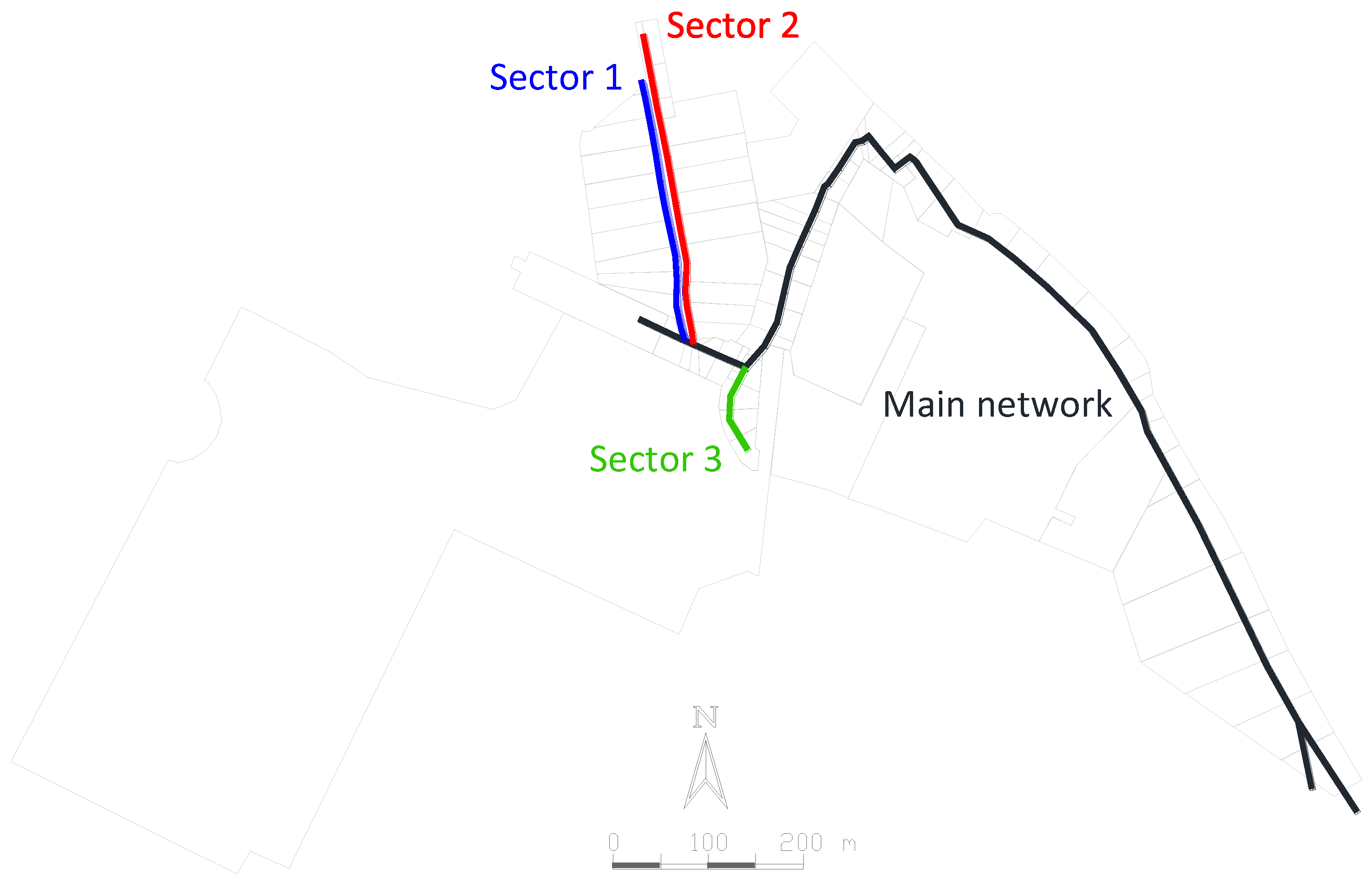
Before applying the SSR method, the sectors that make up the Balloon network and the size of SS are identified. The total network has a magnitude of SS of 233 and 3 sectors are identified that discharge their waters to the main network. Table 1 summarizes the elements that make up each sector, the DVs and the magnitude of SS. Figure 5 shows the sectors and the main network that make up the Balloon network. First, to each of the sectors, the parallel SSR method is applied to decrease the number of DVs. Table 1 also shows the reduction in the magnitude of SS in each of the sectors when applying the clustering method.
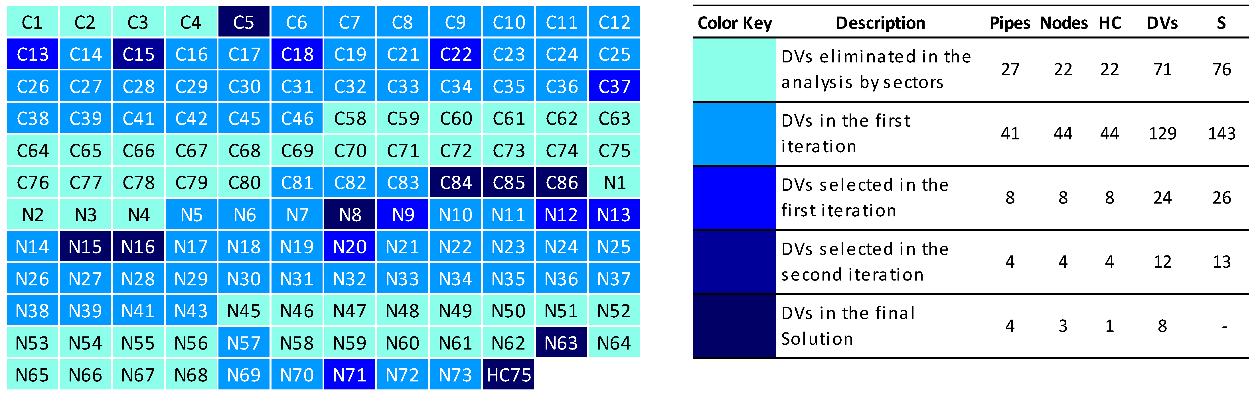
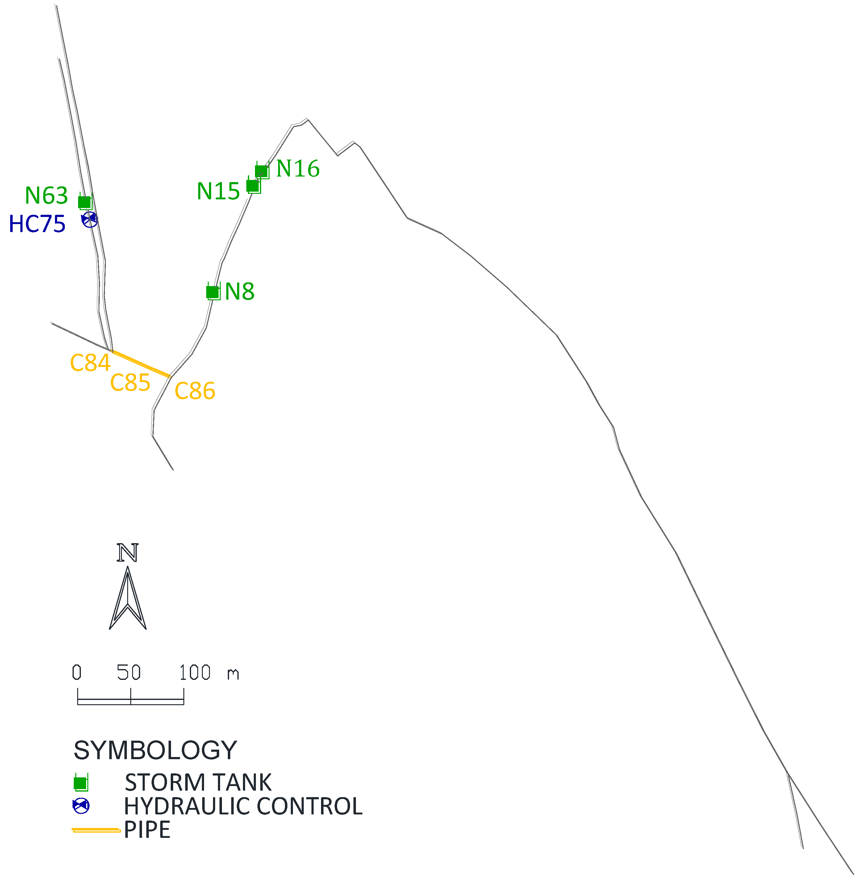
After the initial reduction by sectors, the SSR method is applied to the network iteratively until the final search region is defined. Once the SS is reduced, we proceed to the final optimization, performing a series of simulations to obtain the best possible solution. Figure 11 shows the stages of the SSR in the Balloon network, the number of DVs and the magnitude of SS at each stage of the SSR process, as well as the final solution. Table 2 shows the terms that compose the objective function of the solution found and the characteristics of the elements to be installed. Figure 12 illustrates the elements to be installed in the network.
3.2. ES-N Network
The complete network has an SS magnitude of 1271. Analyzing the problem with the recursive method would demand a very high computational time. For this reason, the SSR clustering method has been considered for the study of the network. As a first step, all the sectors that make up the drainage network are defined. Nineteen sectors have been identified and will be optimized in parallel. Table 3 shows the elements of which the network is composed, the number of DVs and the magnitude of SS. By analyzing the network by sectors and in parallel, it is possible to appreciate the decrease in the magnitude of SS that the algorithm must explore in each scenario. If, in addition to this, it is considered that, in the SSR process, the coarse option lists are used, the computational effort is notably reduced.
For better visualization, the sectors of the drainage network and the main network are differentiated in Figure 7. Applying the SSR method to each sector reduces the number of DVs considerably. The method is applied iteratively until SS cannot be reduced. Table 3 shows the percentage reduction in SS magnitude.
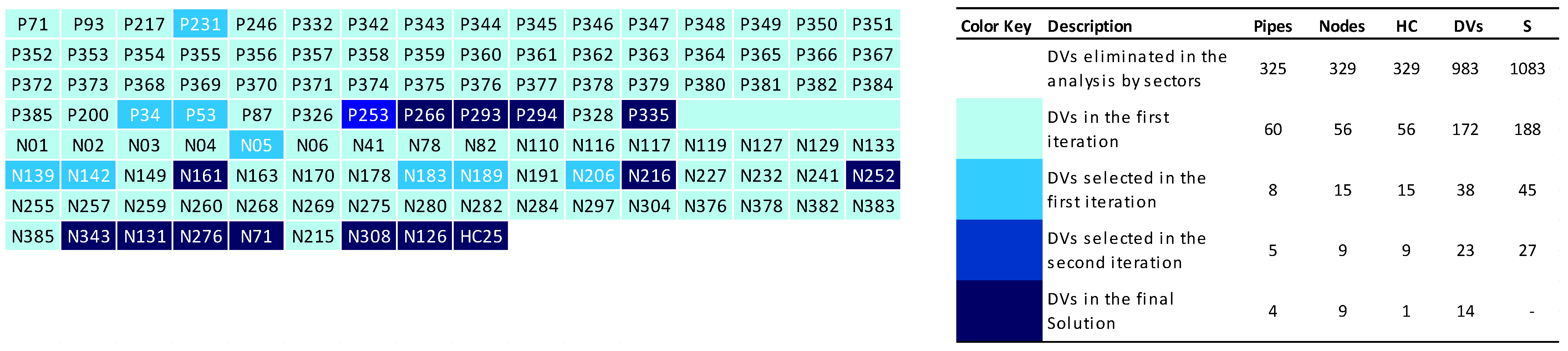
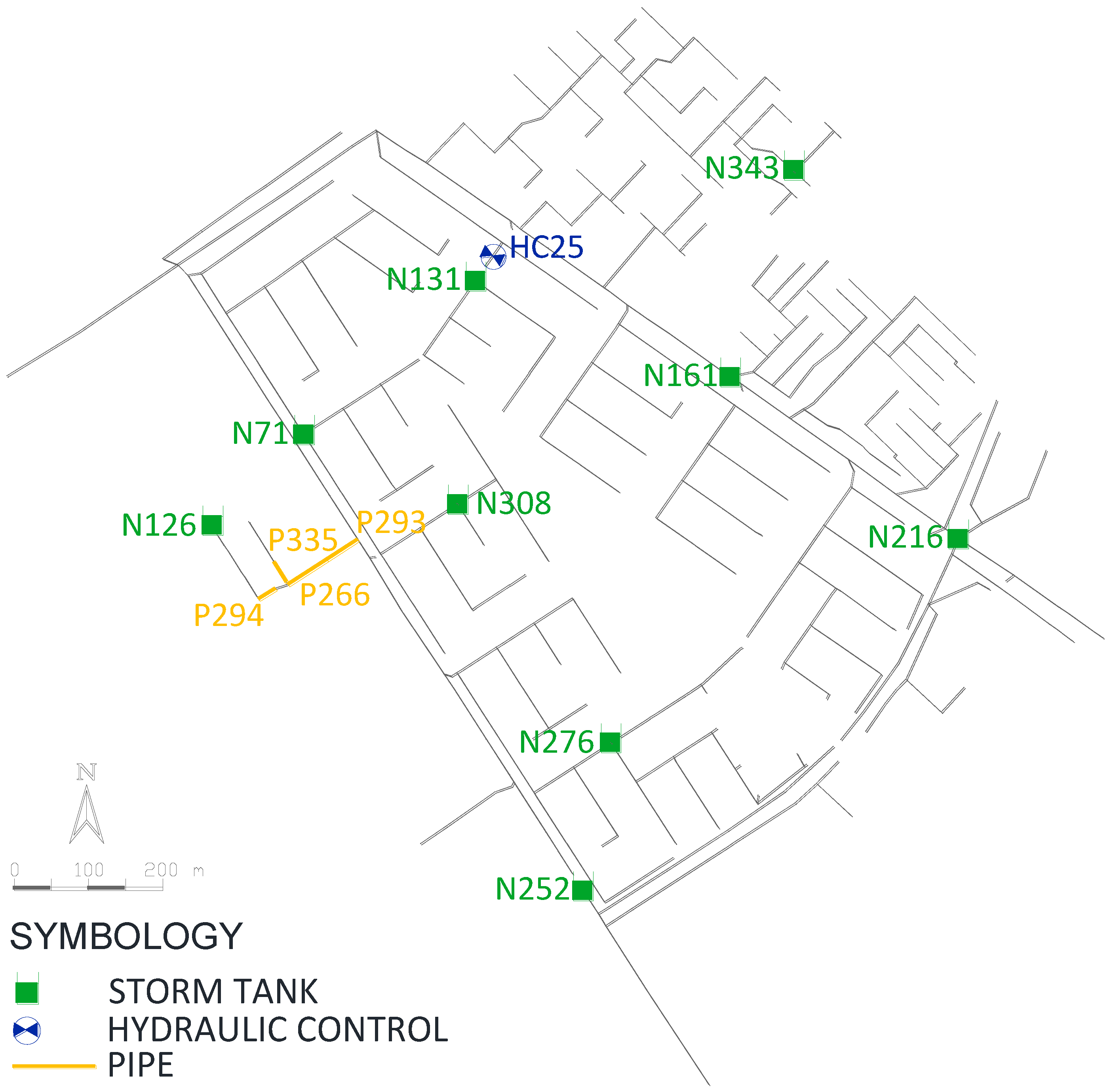
After the application of the SSR in each sector, a new scenario is configured for the optimization of the network that includes the selected DVs in each sector and in the main network. Applying the method in this scenario iteratively defines the final search region. Later, for the final optimization, a refined list of options for the STs is used and the hydraulic control elements are included in the search. At this stage, a much more demanding stopping criterion for the algorithm is also used to find the solution close to the optimal value. After performing a series of simulations, the best possible solution is obtained. Figure 13 shows the SSR until the final solution is found. Table 4 shows the terms that compose the objective function of the solution found and the characteristics of the elements to be implemented. Figure 14 illustrates the elements to be installed in the network. Finally, the dispersion of the different results obtained from the objective function in each iteration and the number of DVs in the case study networks are shown in Figure 15.
4. Discussion
In the optimization process, it is desirable to have a strategy that reduces calculation times, especially when large networks are analyzed. The SSR method used is applied in two networks presented as case studies. In the case of the Balloon network, the network does not have many sectors that make up the drainage network, identifying three sectors. In the process of reduction by sectors, the SS is reduced by 37%. Then, in the iterative analysis with the complete network, it is possible to reduce the SS up to 94%. On the other hand, the ES-N network has the characteristic of being made up of 19 sectors that discharge water to the main network of the drainage network. In this network, the clustering method is applied for the parallel reduction of SS in the analysis stage by sectors; SS is reduced by 85%, this being the great advantage of this methodology: that when analyzing in parallel, a smaller number of DVs are obtained faster. Finally, the SS is reduced to 97.88% in two subsequent iterations. These results show us that the method is particularly beneficial when networks composed of several sectors are analyzed, this being a characteristic of large networks. The process of reducing the SS must prioritize the identification of the best areas of the SS. Figure 15 shows how, when reducing the search region to the most prominent areas, the values of the objective function obtained decrease. It can also be observed how the dispersion of results decreases in each iteration. This can show us that the procedure meets its objective. The results of the final optimization, in economic terms, show the cost of the annual investment prorated throughout the design period and the expected cost that the flood may generate annually. In the Balloon network, losses of 733,282 euros per year are currently generated. When the optimization is carried out, the expected cost of these damages is reduced to 5608 euros per year. On the other hand, in the ES-N network, without making any improvements to the network, rains can be expected to generate damages of 118,955 euros per year. With the implementation of the infrastructure according to the solution found, these damages can be reduced to 27,722 euros per year. If it is considered that the required investment in infrastructure is 3% and 38%, respectively, of the current flood risk costs, it can be said that these investments are relatively low and allow us to verify the advantages of this type of rehabilitation in drainage networks.
5. Conclusions
There are different methods to improve drainage networks. In this work, a methodology based on the substitution of drainage networks combined with the installation of STs and HCs is proposed. The case studies analyzed show the benefits of the method over the traditional pipe replacement technique, since when combined with the installation of STs in line and with the use of HCs, the slowing down of the water is encouraged, reducing the peak of the water flow. In relation to the use of STs in line, it can be said that they have an advantage over traditional STs that are designed to contain a larger volume of water and then require pumping systems to dislodge the water from the tank. With the STs in line, what is sought is a temporary storage of the water to reduce the speed of accumulation downstream. These advantages are explained in detail by Bayas-Jiménez et al. [12]. The use of genetic algorithms is presented as one of the most suitable alternatives to find solutions to this type of problem. Although it is true that its use entails a significant use of resources, there are techniques that can reduce the calculation time. The method presented in this work was previously presented by Bayas-Jiménez et al. [14]. The results obtained in the analyzed case studies show us the suitability of this method. Although the method does not allow a direct reduction of the SS and requires its application in an iterative way, it allows us to address a problem that, without this reduction, would require enormous computational efforts. It should be noted that this method allows rapid convergence towards the best search region. If the results of the first iteration of the SRR process are analyzed, it can be seen how a large amount of the search space is quickly eliminated.
The analysis of the problem focused on evaluating the problem in economic terms, quantifying the cost that the flood would produce in the cities. The analysis fundamentally depends on the volume of flood water that is generated. Analyzing the problem using a design rainfall for the return period used for the design of the network may, at first sight, be the best alternative to the problem. By using this design rainfall, the situation that makes the greatest demands on the operation of the network can be analyzed. However, this form of analysis does not analyze other minor rains that may appear during the period of operation of the network and that can generate floods in the network that, although minor, are not accounted for in the analyzed objective function. The approach used in this work has tried to solve this problem. By analyzing the costs on an annualized basis based on an annual estimate of the damage, it is possible to have a clearer idea of the cost of the damages that the risk of flooding implies. In any case, it must be taken into account that this method is approximate, and that the results will depend greatly on the number of storms analyzed. It is noteworthy to mention that this work does not contemplate in its objectives the realization of projections of increased rainfall due to the effects of climate change. However, if you wanted to analyze a network under this scenario, the methodology could be applied without problems.
On the other hand, identifying different land uses in the studied areas allows for a better optimization of the networks compared to the use of an average curve for the entire study area, as has been done in previous works; this is undoubtedly an improvement that this work presents to the developed methodology. However, this additional action demands longer calculation times, so the use of an SSR method becomes unavoidable.
Finally, distinguishing different zones within the study area and the cost that a flood would entail in that place allows greater protection to be given to particularly sensitive zones or strategies in the functioning of the city. In contrast, in areas where a flood would not cause serious problems, for example, in green areas, a greater volume of flooding can be allowed. This would allow linking the present study to the joint analysis with low-impact developments (LIDs) techniques in specific areas of the cities in which these techniques can be included. This study is proposed as a future development in this line of research.
Supplementary Materials
The following supporting information can be downloaded at: https://www.mdpi.com/article/10.3390/w14182901/s1, Figure S1: Representation of Balloon drainage network; Figure S2: Representation of ES-N drainage network. Table S1: Data for nodes and subcatchments of Balloon network; Table S2: Data for conduits in the network used as a case study; Table S3: Land uses in the study area of Balloon network; Table S4: Data for nodes and subcatchments in the ES-N network; Table S5: Data for pipes in the ES-N network; Table S6: Land uses in the study area of ES-N network; Table S7: Goodness of fit for the different land uses with Equation (5); Table S8: Coefficients of Equation (5) for different land uses.
Author Contributions
All authors contributed extensively to the work presented in this paper. Conceptualization, L.B.-J., F.J.M.-S. and P.L.I.-R.; data curation, L.B.-J. and F.J.M.-S.; formal analysis, L.B.-J., F.J.M.-S., P.L.I.-R. and F.B.; funding acquisition L.B.-J. and F.J.M.-S.; investigation, L.B.-J., F.J.M.-S., P.L.I.-R. and F.B.; methodology L.B.-J., F.J.M.-S. and P.L.I.-R.; project administration, L.B-J. and F.J.M.-S.; resources, L.B.-J., F.J.M.-S., P.L.I.-R. and F.B.; software, L.B.-J., F.J.M.-S. and P.L.I.-R.; supervision, F.J.M.-S., P.L.I.-R. and F.B.; validation, L.B.-J., F.J.M.-S., P.L.I.-R. and F.B.; visualization, L.B.-J., F.J.M.-S., P.L.I.-R. and F.B.; writing—original draft, L.B.-J., F.J.M.-S., P.L.I.-R. and F.B.; writing—review and editing, L.B.-J., F.J.M.-S., P.L.I.-R. and F.B. All authors have read and agreed to the published version of the manuscript.
Funding
The APC was funded by the Universitat Politècnica de València.
Data Availability Statement
Not applicable.
Conflicts of Interest
The authors declare no conflict of interest.
Abbreviations
The following abbreviations are used in this manuscript:
| DV | Decision Variable |
| EAD | Estimated Annual Damage |
| IDF | Intensity–Duration–Frequency |
| LID | Low-Impact Development |
| OF | Objective Function |
| PGA | Pseudo-Genetic Algorithm |
| SS | Search Space |
| SSR | Search Space Reduction |
| SWMM | Storm Water Management Model |
| Nomenclature | |
| a | coefficient of the line of the flood cost |
| Ai | flood area |
| b | coefficient of the line of the flood cost |
| Cmax | maximum flood damage cost |
| Cmin | minimum cost of building a storm tank |
| CP (Di) | cost of pipe replacement |
| CT (Vi) | cost of building a storm tank |
| Cv (Di) | cost of installing hydraulic controls |
| Cvar | adjustment coefficient for calculating the cost of storm tank |
| Cy (yi) | flood damage cost |
| Di | pipe diameter |
| Gmax | convergence criterion |
| Li | pipe length |
| ms | pipes selected to be optimized |
| NDmax | diameter range available |
| ns | nodes selected to be optimized |
| NS | list of options used for nodes |
| NSmax | refined option list for nodes |
| NS0 | coarse option list for nodes |
| Nθ | option list for hydraulic controls |
| p | annual exceedance rate |
| p0 | annual exceedance rate for which flood damage begins to occur |
| r | annual interest |
| t | years to recover the investment |
| T | return period |
| Vi | flood volume at the node |
| vs | pipes selected to install hydraulic controls in the optimization process |
| yi | flood depth at node |
| ymax | maximum depth at which the maximum cost of flood damage is reached |
| α | adjustment coefficient for calculating the cost of replacing pipes |
| β | adjustment coefficient for calculating the cost of replacing pipes |
| γ | adjustment coefficient for calculating the cost of replacing pipes |
| ΔND | range of diameters immediately larger than the analyzed pipe |
| Λ | annual amortization factor |
| λ | adjustment coefficient for calculation of flood damage |
| μ | adjustment coefficient for calculating the cost of installing hydraulic controls |
| σ | adjustment coefficient for calculating the cost of installing hydraulic controls |
| υ | adjustment coefficient for calculation of flood damage |
| φ | adjustment coefficient for calculating the cost of installing hydraulic controls |
| ω | adjustment constant for the calculation of the cost of the construction of storm tanks |
References
- Xiong, L.; Yan, L.; Du, T.; Yan, P.; Li, L.; Xu, W. Impacts of Climate Change on Urban Extreme Rainfall and Drainage Infrastructure Performance: A Case Study in Wuhan City, China. Irrig. Drain. 2019, 68, 152–164. [Google Scholar] [CrossRef]
- Salinas-Rodriguez, C.; Gersonius, B.; Zevenbergen, C.; Serrano, D.; Ashley, R. A Semi Risk-Based Approach for Managing Urban Drainage Systems under Extreme Rainfall. Water 2018, 10, 384. [Google Scholar] [CrossRef]
- Szewrański, S.; Chruściński, J.; Kazak, J.; Świąder, M.; Tokarczyk-Dorociak, K.; Żmuda, R. Pluvial Flood Risk Assessment Tool (PFRA) for Rainwater Management and Adaptation to Climate Change in Newly Urbanised Areas. Water 2018, 10, 386. [Google Scholar] [CrossRef]
- Oberascher, M.; Kinzel, C.; Kastlunger, U.; Kleidorfer, M.; Zingerle, C.; Rauch, W.; Sitzenfrei, R. Integrated urban water management with micro storages developed as an IoT-based solution—The smart rain barrel. Environ. Model. Softw. 2021, 139, 105028. [Google Scholar] [CrossRef]
- Szeląg, B.; Suligowski, R.; De Paola, F.; Siwicki, P.; Majerek, D.; Łagód, G. Influence of urban catchment characteristics and rainfall origins on the phenomenon of stormwater flooding: Case study. Environ. Model. Softw. 2022, 150, 105335. [Google Scholar] [CrossRef]
- Olcina, J.; Hernández, M.; Morote, Á.-F.; Eslamian, S. Reducing Flood Risk in Spain: The Role of Spatial Planning. In Flood Handbook, 1st ed.; Eslamian, S., Eslamian, F.A., Eds.; CRC Press: Boca Raton, FL, USA, 2022; pp. 217–226. [Google Scholar]
- Meyer, V.; Becker, N.; Markantonis, V.; Schwarze, R.; Van der Bergh, J.C.J.M.; Bouwer, L.M.; Viavattene, C. Review article: Assessing the costs of natural hazards—State of the art and knowledge gaps. Nat. Hazards Earth Syst. Sci. 2013, 13, 1351–1373. [Google Scholar] [CrossRef]
- Nicklin, H.; Leicher, A.M.; Dieperink, C.; Van Leeuwen, K. Understanding the Costs of Inaction—An Assessment of Pluvial Flood Damages in Two European Cities. Water 2019, 11, 801. [Google Scholar] [CrossRef]
- Mobini, S.; Nilsson, E.; Persson, A.; Becker, P.; Larsson, R. Analysis of pluvial flood damage costs in residential buildings—A case study in Malmö. Int. J. Disaster Risk Reduct. 2021, 62, 102407. [Google Scholar] [CrossRef]
- O’Donnell, E.C.; Thorne, C.R. Drivers of future urban flood risk. Philos. Trans. R. Soc. A Math. Phys. Eng. Sci. 2020, 378, 20190216. [Google Scholar] [CrossRef]
- Andrés-Doménech, I.; Montanari, A.; Marco, J.B. Efficiency of storm detention tanks for urban drainage systems under climate variability. J. Water Resour. Plan. Manag. 2012, 138, 36–46. [Google Scholar] [CrossRef]
- Bayas-Jiménez, L.; Martínez-Solano, F.J.; Iglesias-Rey, P.L.; Mora-Melia, D.; Fuertes-Miquel, V.S. Inclusion of Hydraulic Controls in Rehabilitation Models of Drainage Networks to Control Floods. Water 2021, 13, 514. [Google Scholar] [CrossRef]
- Maier, H.R.; Kapelan, Z.; Kasprzyk, J.; Kollat, J.; Matott, L.S.; Cunha, M.C.; Reed, P.M. Evolutionary algorithms and other metaheuristics in water resources: Current status, research challenges and future directions. Environ. Model. Softw. 2014, 62, 271–299. [Google Scholar] [CrossRef]
- Bayas-Jiménez, L.; Martínez-Solano, F.J.; Iglesias-Rey, P.L.; Mora-Meliá, D. Search space reduction for genetic algorithms applied to drainage network optimization problems. Water 2021, 13, 2008. [Google Scholar] [CrossRef]
- Marchi, A.; Salomons, E.; Ostfeld, A.; Kapelan, Z.; Simpson, A.; Zecchin, A.; Maier, H.; Wu, Z.; Elsayed, S.M.; Song, Y.; et al. Battle of the Water Networks II. J. Water Resour. Plan. Manag. 2014, 140, 04014009. [Google Scholar] [CrossRef]
- Mora, D. Design of Water Distribution Networks Using Evolutionary Algorithms. Efficiency Analysis. Ph.D. Thesis, Universitat Politècnica de València, Valencia, Spain, July 2012. (In Spanish). [Google Scholar]
- Schraudolph, N.N.; Belew, R.K. Dynamic Parameter Encoding for Genetic Algorithms. Mach. Learn. 1992, 9, 9–21. [Google Scholar] [CrossRef]
- Sophocleous, S.; Savić, D.; Kapelan, Z. Leak Localization in a Real Water Distribution Network Based on Search-Space Reduction. J. Water Resour. Plan. Manag. 2019, 145, 04019024. [Google Scholar] [CrossRef]
- Freni, G.; La Loggia, G.; Notaro, V. Uncertainty in urban flood damage assessment due to urban drainage modelling and depth-damage curve estimation. Water Sci. Technol. 2010, 61, 2979–2993. [Google Scholar] [CrossRef]
- Zhou, Q.; Mikkelsen, P.S.; Halsnæs, K.; Arnbjerg-Nielsen, K. Framework for economic pluvial flood risk assessment considering climate change effects and adaptation benefits. J. Hydrol. 2012, 414, 539–549. [Google Scholar] [CrossRef]
- Olsen, A.S.; Zhou, Q.; Linde, J.J.; Arnbjerg-Nielsen, K. Comparing methods of calculating expected annual damage in urban pluvial flood risk assessments. Water 2015, 7, 255–270. [Google Scholar] [CrossRef]
- Mora-Melia, D.; Iglesias-Rey, P.L.; Martinez-Solano, F.J.; Fuertes-Miquel, V.S. Design of Water Distribution Networks using a Pseudo-Genetic Algorithm and Sensitivity of Genetic Operators. Water Resour. Manag. 2013, 27, 4149–4162. [Google Scholar] [CrossRef]
- Rossman, L.A. Storm Water Management Model (SWMM) User’s Manual Version 5.0; U.S. EPA: Cincinnati, OH, USA, 2009. [Google Scholar]
- Martínez-Solano, F.J.; Iglesias-Rey, P.L.; Saldarriaga, J.G.; Vallejo, D. Creation of an SWMM toolkit for its application in urban drainage networks optimization. Water 2016, 8, 259. [Google Scholar] [CrossRef]
- Locatelli, L.; Guerrero, M.; Russo, B.; Martínez-Gomariz, E.; Sunyer, D.; Martínez, M. Socio-Economic Assessment of Green Infrastructure for Climate Change Adaptation in the Context of Urban Drainage Planning. Sustainability 2020, 12, 3792. [Google Scholar] [CrossRef]
- Arnell, N.W. Expected Annual Damages and Uncertainties in Flood Frequency Estimation. J. Water Resour. Plan. Manag. 1989, 115, 94–107. [Google Scholar] [CrossRef]
- Butler, D.; Digman, C.J.; Makropoulos, C.; Davies, J.W. Urban Drainage, 4th ed.; CRC Press, Taylor & Francis Group: Boca Raton, FL, USA, 2018. [Google Scholar]
- Arnbjerg-Nielsen, K.; Fleischer, H.S. Feasible adaptation strategies for increased risk of flooding in cities due to climate change. Water Sci. Technol. 2009, 60, 273–281. [Google Scholar] [CrossRef] [PubMed]
- Reca, J.; Martínez, J.; López, R. A Hybrid Water Distribution Networks Design Optimization Method Based on a Search Space Reduction Approach and a Genetic Algorithm. Water 2017, 9, 845. [Google Scholar] [CrossRef]
- Creaco, E.; Pezzinga, G. Embedding linear programming in multi objective genetic algorithms for reducing the size of the search space with application to leakage minimization in water distribution networks. Environ. Model. Softw. 2015, 69, 308–318. [Google Scholar] [CrossRef]
- Kadu, M.S.; Gupta, R.; Bhave, P.R. Optimal Design of Water Networks Using a Modified Genetic Algorithm with Reduction in Search Space. J. Water Resour. Plan. Manag. 2008, 134, 147–160. [Google Scholar] [CrossRef]
- Martínez-Gomariz, E.; Gómez, M.; Russo, B.; Sánchez, P.; Montes, J.-A. Methodology for the damage assessment of vehicles exposed to flooding in urban areas. J. Flood Risk Manag. 2019, 12, e12475. [Google Scholar] [CrossRef]
Figure 1.
Damage–Depth curve (a), Damage—annual exceedance rate curve (b) and Flood risk density curve (c).
Figure 1.
Damage–Depth curve (a), Damage—annual exceedance rate curve (b) and Flood risk density curve (c).

Figure 2.
Schematic diagram of the optimization model.

Figure 3.
Annual cost of flood risk as the area under the curve in a log-linear relationship.

Figure 4.
Drainage network with identification of branches and main network.

Figure 5.
Balloon Network.

Figure 6.
IDF Curves studied for Balloon network.

Figure 7.
ES-N Network.

Figure 8.
IDF curves studied for ES-N network.

Figure 9.
Cost curves of pipelines, STs and HCs for the case study.

Figure 10.
Damage–depth curve for the case study.

Figure 11.
SSR in Balloon network.

Figure 12.
Location of infrastructure needed to rehabilitate the Balloon network.

Figure 13.
SSR in the ES-N network.

Figure 14.
Location of infrastructure needed to rehabilitate the ES-N network.

Figure 15.
Results of the Objective Function in each iteration analyzed. (a) Balloon network. (b) ES-N network.
Figure 15.
Results of the Objective Function in each iteration analyzed. (a) Balloon network. (b) ES-N network.


Table 1.
Elements, magnitude of SS and percentage of reduction of the sectors that make up the Balloon network.
Table 1.
Elements, magnitude of SS and percentage of reduction of the sectors that make up the Balloon network.
| Sector | Number of Pipes | Number of Nodes | DV | SS | Reduction of SS in Clustering Process |
|---|---|---|---|---|---|
| Sector 1 | 11 | 11 | 33 | 36 | 100% |
| Sector 2 | 12 | 12 | 36 | 40 | 96% |
| Sector 3 | 4 | 4 | 12 | 13 | 100% |
| Main network | 44 | 43 | 130 | 144 | |
| Total | 71 | 70 | 211 | 233 |
Table 2.
Results of the final optimization in the Balloon network.
| Terms in Objective Function | Pipes | Storm Tank | Hydraulic Control | Flood | Total | ||||||
|---|---|---|---|---|---|---|---|---|---|---|---|
| Cost per year | 2739 € | 19,727 € | 153 € | 5608 € | 28,227 € | ||||||
| Elements | C5 | C84 | C85 | C86 | N8 | N15 | N16 | N63 | C75 | ||
| Present diameter (m) | 0.70 | 0.70 | 0.70 | 0.70 | |||||||
| Optimized diameter (m) | 1.00 | 1.10 | 1.00 | 1.00 | |||||||
| Volume (m3) | 2496 | 4284 | 5031 | 594 | |||||||
| Head-loss (m) | 72.55 | ||||||||||
Table 3.
Elements, magnitude of SS and percentage of reduction in the clustering stage of the sectors that make up the ES-N network.
Table 3.
Elements, magnitude of SS and percentage of reduction in the clustering stage of the sectors that make up the ES-N network.
| Sector | Number of Pipes | Number of Nodes | DVs | SS | Reduction of SS in Clustering Process |
|---|---|---|---|---|---|
| Sector 1 | 5 | 5 | 15 | 17 | 100% |
| Sector 2 | 2 | 2 | 6 | 7 | 100% |
| Sector 3 | 13 | 13 | 39 | 43 | 100% |
| Sector 4 | 23 | 23 | 69 | 76 | 98% |
| Sector 5 | 24 | 24 | 72 | 79 | 91% |
| Sector 6 | 8 | 8 | 24 | 26 | 100% |
| Sector 7 | 55 | 55 | 165 | 182 | 99% |
| Sector 8 | 8 | 8 | 24 | 26 | 100% |
| Sector 9 | 15 | 15 | 45 | 50 | 100% |
| Sector 10 | 23 | 23 | 69 | 76 | 100% |
| Sector 11 | 25 | 25 | 75 | 83 | 100% |
| Sector 12 | 16 | 16 | 48 | 53 | 97% |
| Sector 13 | 9 | 9 | 27 | 30 | 100% |
| Sector 14 | 5 | 5 | 15 | 17 | 100% |
| Sector 15 | 39 | 39 | 117 | 129 | 97% |
| Sector 16 | 45 | 45 | 135 | 149 | 97% |
| Sector 17 | 4 | 4 | 12 | 13 | 100% |
| Sector 18 | 12 | 12 | 36 | 40 | 75% |
| Sector 19 | 5 | 5 | 15 | 17 | 100% |
| Main network | 49 | 49 | 147 | 162 | |
| Total | 385 | 385 | 1155 | 1271 |
Table 4.
Objective function of the best solution found for the ES-N network.
| Terms in Objective Function | Pipes | Storm Tank | Hydraulic Control | Flood | Total | |||||||
|---|---|---|---|---|---|---|---|---|---|---|---|---|
| Cost per year | 2672 € | 41,930 € | 125 € | 27,722 € | 72,449 € | |||||||
| Elements | P266 | P293 | P294 | P335 | N71 | N126 | N131 | N161 | N216 | P25 | ||
| N252 | N276 | N308 | N343 | |||||||||
| Present diameter (m) | 0.40 | 0.40 | 0.25 | 0.30 | ||||||||
| Optimized diameter (m) | 0.70 | 0.70 | 0.45 | 0.50 | ||||||||
| Volume (m3) | 1700 | 500 | 750 | 1950 | 1950 | |||||||
| 1100 | 1250 | 1050 | 800 | |||||||||
| Head-loss (m) | 72.55 | |||||||||||
Publisher’s Note: MDPI stays neutral with regard to jurisdictional claims in published maps and institutional affiliations. |
© 2022 by the authors. Licensee MDPI, Basel, Switzerland. This article is an open access article distributed under the terms and conditions of the Creative Commons Attribution (CC BY) license (https://creativecommons.org/licenses/by/4.0/).
Share and Cite
MDPI and ACS Style
Bayas-Jiménez, L.; Martínez-Solano, F.J.; Iglesias-Rey, P.L.; Boano, F. Economic Analysis of Flood Risk Applied to the Rehabilitation of Drainage Networks. Water 2022, 14, 2901. https://doi.org/10.3390/w14182901
AMA Style
Bayas-Jiménez L, Martínez-Solano FJ, Iglesias-Rey PL, Boano F. Economic Analysis of Flood Risk Applied to the Rehabilitation of Drainage Networks. Water. 2022; 14(18):2901. https://doi.org/10.3390/w14182901
Chicago/Turabian StyleBayas-Jiménez, Leonardo, F. Javier Martínez-Solano, Pedro L. Iglesias-Rey, and Fulvio Boano. 2022. "Economic Analysis of Flood Risk Applied to the Rehabilitation of Drainage Networks" Water 14, no. 18: 2901. https://doi.org/10.3390/w14182901
Note that from the first issue of 2016, this journal uses article numbers instead of page numbers. See further details here.