
Enhancing a Multi-Step Discharge Prediction with Deep Learning and a Response Time Parameter

1
Department of Water Resources Engineering, Kasetsart University, Bangkok 10900, Thailand
2
Department of Industrial Engineering, Kasetsart University, Bangkok 10900, Thailand
*
Author to whom correspondence should be addressed.
Water 2022, 14(18), 2898; https://doi.org/10.3390/w14182898
Submission received: 11 August 2022
/
Revised: 8 September 2022
/
Accepted: 13 September 2022
/
Published: 16 September 2022
(This article belongs to the Section Hydrology)
Abstract
:Flood forecasting is among the most important precaution measures to prevent devastating disasters affecting human life, properties, and the overall environment. It is closely involved with precipitation and streamflow data forecasting tasks. In this work, we introduced a multi-step discharge prediction framework based on deep learning models. A simple feature representation technique using a correlation of backward lags was enhanced with a time of concentration (TC) concept. Recurrent neural networks and their variants, coupled with the TC-related features, provided superior performance with over 0.9 Nash–Sutcliffe model efficiency coefficient and substantially high correlation values for multiple forecasted points. These results were consistent among both the Upper Nan and the Loei river basins in Thailand, which were used as case studies in this work.
1. Introduction
The global population continues to grow every year, leading to an intense requirement for a well-managed water system. Inefficient land-use management coupled with external factors such as climate change could be one of the root causes of flood events. Floods are among the most damaging natural disasters, which could negatively affect a wide range of people and the entire nation including Thailand [1]. Flood control is critical in terms of lessening devastating effects on human life, livelihood as well as properties. More importantly, flood forecasting and an early warning system are required to prevent or minimize risks in flood-prone areas [2,3]. These systems rely mainly on precipitation and streamflow data to predict the water level data, especially abrupt rises leading to flooding events.
With advanced technologies, Artificial Intelligence (AI), Machine Learning (ML), and Deep Learning (DL) have been applied to various domains to analyze and extract insights from historical data. These data-driven methodologies have also gained popularity in hydrology applications. Chang et al. [4] explored the state-of-the-art ML research focusing on flood forecasts with diverse case studies. In earlier days, various ML models were popular and effective in providing accurate flood forecasting results. However, these ML methods mostly require significant effort in manually generating insightful features. To address this, Artificial Neural Networks (ANNs) mimicking neurons in a human brain were developed at an early age of DL. They were built on more complicated interconnections among nodes from multiple layers of the networks. Several models and their variations have been applied to the flood forecasting tasks, as highlighted in [5,6,7,8,9,10]. In addition, river flow forecasting using artificial intelligence is among the fundamental components of water resources management [11]. For example, common ML models such as Support Vector Regression (SVR), Random Forest (RF), ANNs, and Extreme Learning Machine (ELM) were employed to estimate monthly and daily river streamflow, see [12,13]. Rezaie-Balf et al. [14] proposed a hybrid decomposition-based AI for daily streamflow prediction which was superior to individual models.
Later on, the focus of model development shifted to deep learning methods, especially with rich data. Recurrent Neural Networks (RNNs) and their variations have gained popularity over the past years to tackle sequence input like time series data or textual data within natural language processing applications. With specifically-designed network architectures, RNNs can extract features from the original sequence input. They are also widely used in hydrology to predict water levels in advance for flood control [15,16]. Thereafter, more advanced model architectures based on RNNs were developed. Specifically, Gated Recurrent Units (GRUs) and Long Short-Term Memory Networks (LSTMs) handled short-term memory with gate mechanisms within the networks to control the flow of information. Among these models, LSTMs and their variants were the most popular methods in hydrology due to their capability of long-term dependency learning. For instance, LSTM models were utilized for flood forecasting as introduced in previous studies [17,18,19,20,21]. Furthermore, Apaydin et al. [22] proposed a thorough comparative analysis of RNNs for reservoir inflow forecasting.
The classical method for flood hydrograph analysis typically requires time parameters of catchment response such as the time of concentration (TC), lag time (TL), and Time to peak (TP). These parameters are normally used to indicate the catchment characteristics, direct runoff as well as effective rainfall distribution [23]. The Tc concept is commonly employed to define the required time of runoff contributing to the peak discharge from the catchment boundary to the outlet [24]. Many empirical equations have been proposed to estimate TC [23,25,26,27,28,29]. Each equation represented selected study areas that were related to the geomorphology and climatology of the catchment. Both overland flow and channel flow were considered in the stepwise multiple regression analysis [25,30,31]. The Tc parameter was widely applied for various flood analyses such as flood quantity prediction [32], flood routing in channels [33], and flood design of a drainage system [31]. Gericke and Smithers [24] reviewed methods to evaluate the catchment response time for a flood peak estimation in South Africa. Specifically, TC was so frequently used that it became the required time parameter in the flood hydrograph estimation. The NRCS velocity method, developed by the Natural Resources Conservation Service (NRCS), is commonly used to estimate Tc for both overland flow and/or channel flow [24,34,35]. With channel flow, the NRCS velocity method divides the flow path into segments of uniform hydraulic characteristics. Travel time calculations of water discharge are conducted for each segment which is further summarized as the final TC value.
In this study, we proposed a discharge estimation model for flood forecasting and early warning system. Specifically, our multi-step forecasting model predicted every point of discharge value for the next 12 h. This forecasting horizon was specifically selected based on the flood warning guideline of the Royal Irrigation Department (RID) for both study areas. Thorough processing steps, consisting of data collection, data preparation, model development, and model evaluation, were carefully conducted. Highly correlated lags were experiments in the data preparation step. In addition, the Tc concept, commonly used for flood hydrograph prediction, was further incorporated to derive more insightful information for the model. In the model development process, standard RNNs, GRUs, and LSTMs models were investigated to ensure the networks’ performance. Several evaluation metrics were considered against various models with diverse hyperparameters.
Model experiments with data applications and the TC concept distinguish our work from others. Our main contribution is incorporating the TC concept to capture time lags in the feature generation step. We considered the hydrology knowledge to understand specific catchment characteristics via the Tc concept. Experiments on several models with diverse settings were conducted. To the best of our knowledge, no previous study has directly used the TC concept to predict discharge values using deep learning models. Also, there was no prior work that trained deep learning models using river discharge data in Thailand.
We summarize the primary materials and methods as discussed in Section 2. An overall framework, an experimental analysis, and evaluation metrics used to test the models were elaborated. Results of all experiments and discussions were provided in Section 3. A conclusion is finally stated in the last section.
2. Materials and Methods
In this work, we proposed a novel framework to forecast river discharge data which relied mainly on feature representations and prediction models. We thoroughly experimented on two study areas, including the Upper Nan and the Loei river basins in Thailand. Data preparation and background information of implemented models were also discussed. Common evaluation metrics to measure models’ performances were described.
2.1. Study Area
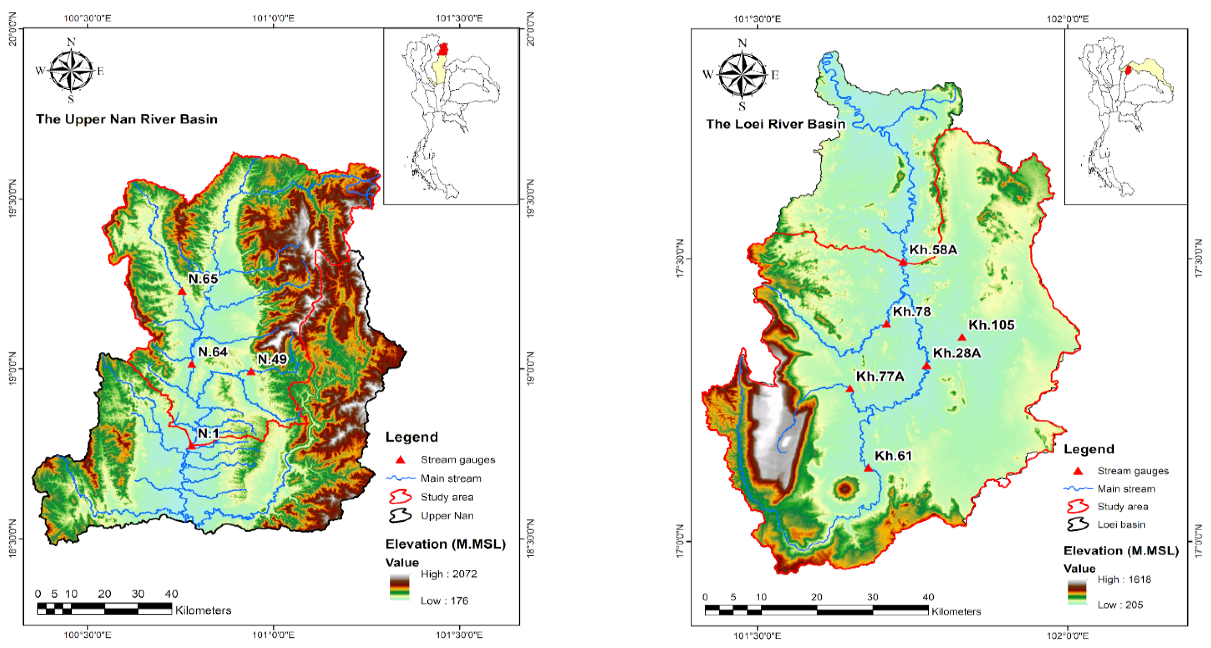
Two study areas in the Upper Nan River basin and the Loei river basin in Thailand are shown in Figure 1. The Upper Nan River basin was in Northern Thailand, with a drainage area of 8706 km2 (4560 km2 of the study area). Annual rainfall and annual runoffs are 1308 mm and 5940 mcm, respectively. Hourly water level data were collected from four stream gauges. Most of the topography of this study area is the mountains and terraced mountains. The major river, named Nan River, originates at a mountain in the north of Nan province and flows through a main economic source in a southern community area. On the other hand, the Loei river basin covers 3956 km2 of the watershed area (3093 km2 of the study area) with 1346 mm of annual rainfall and 1380 mcm of annual runoff. Hourly water level data were collected from six stream gauges. Loei is a sub-basin of the Mekong River basin located in the northeastern region of Thailand. It originates from Phu Luang Mountain and gradually descends to the northern part. The major river, Nam Loei river, flows through the Muang District to meet the Mekong River. Both study areas are affected by the southwest monsoon and tropical depression from the South China Sea during the wet season (May–October).
2.2. Methodology
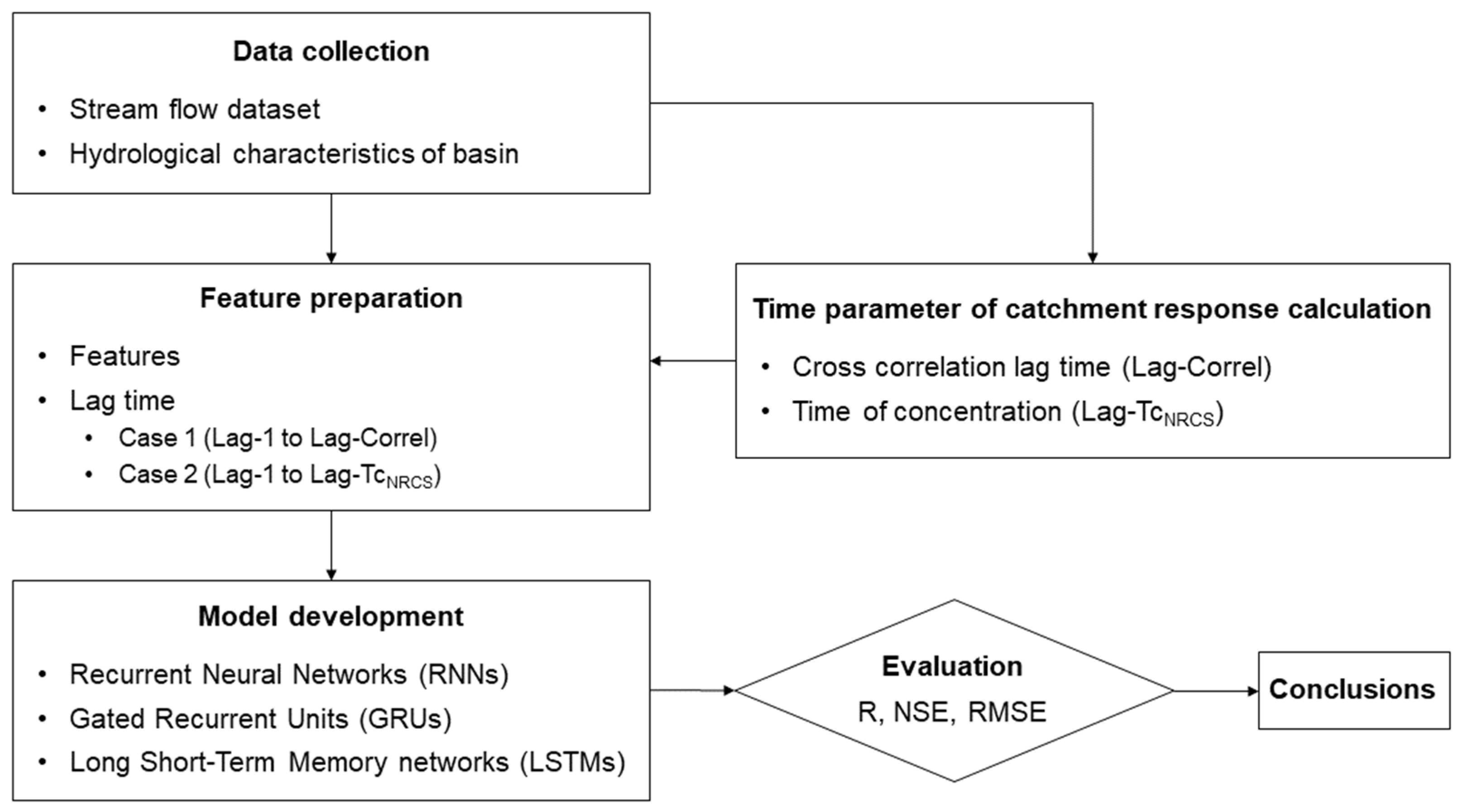
Water level data were collected from multiple telemetry stations in the Upper Nan and the Loei river basins, which were our two case studies in this work. An exploratory data analysis was performed as an initial step of the data preparation process. Missing values and extreme anomalies resulting from malfunctioned sensors or unexpected events were properly pre-processed as explained in the data collection and data preparation section below. Feature representations were carefully prepared using time-lag correlation and the Tc concept. Next, multiple data modeling techniques were implemented and compared with well-defined evaluation metrics. A flow chart of the entire process is summarized in Figure 2.
2.2.1. Data Collection and Data Preparation
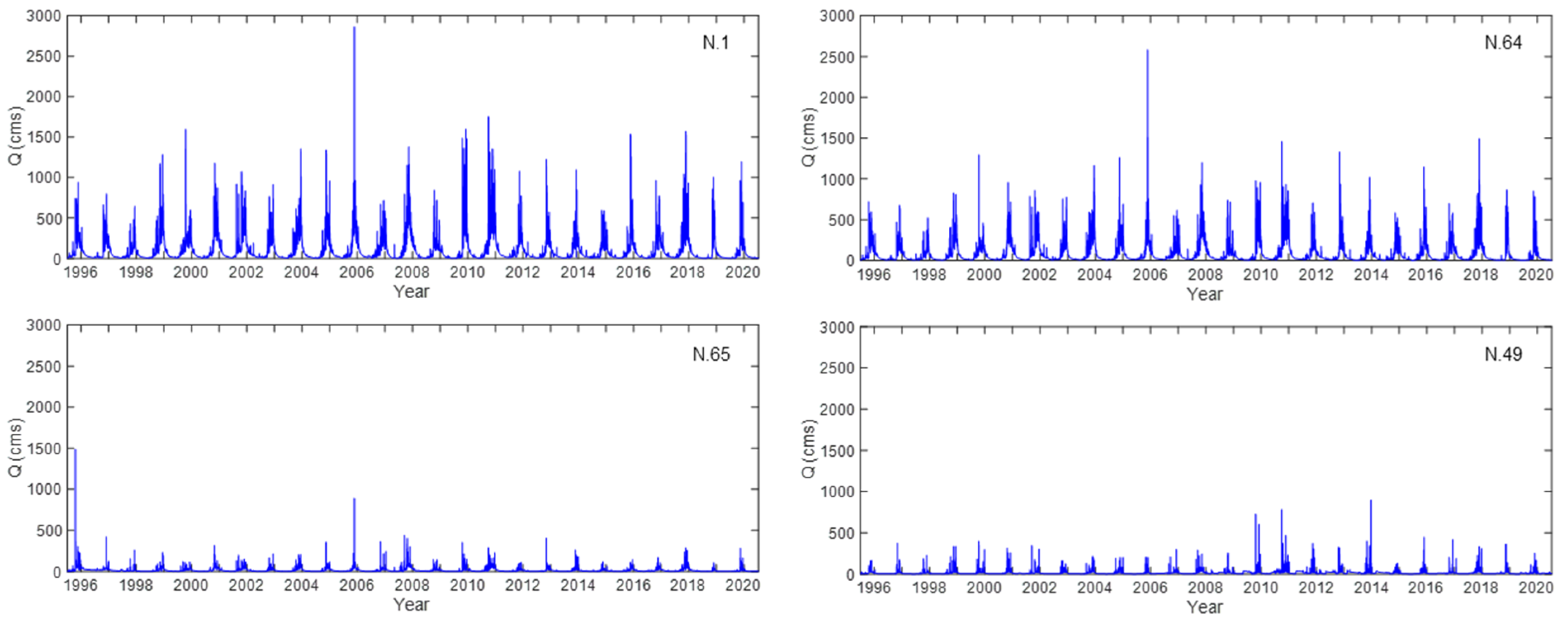
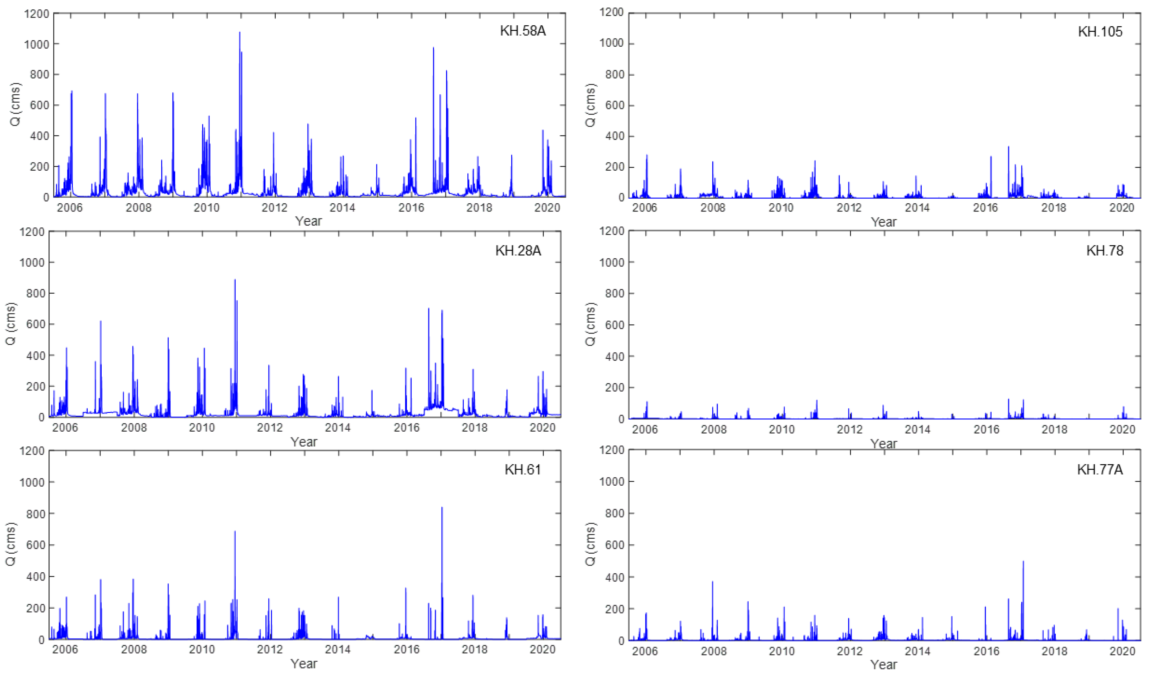
An hourly water level was converted to an hourly discharge by using an annual rating curve. Then, this hourly discharge data at multiple stations corresponding to the Upper Nan and the Loei river basins were explored. A typical outlier detection technique was employed to eliminate extreme anomalies. Specifically, data points that deviated significantly from most of the normal patterns were removed. The remaining incomplete data consisting of missing values and removed outliers were imputed using an interpolation function. An overview of discharge data after the preprocessing step of stations in the Upper Nan and the Loei river basins is illustrated in Figure 3 and Figure 4, respectively.
After the preprocessing step, we split the whole dataset for both study areas into 2 main parts for training, and testing purposes. The entire range of our data was from 1996 to 2020 for the Upper Nan and from 2006 to 2020 for the Loei river basins. Approximately 80 percent of the whole data were used for training while the rest were treated as testing datasets. Furthermore, the training data was partially partitioned into a validation part during the training process to reduce the overfitting circumstances. We intentionally split the data linearly as discharge data was a time series where dependency over time should still be preserved. According to our manual observation, we carefully selected the splitting point to guarantee consistency of seasonal fluctuations and distributions within the data among training and testing parts. This will enhance the possibility that our proposed model should provide a similar accuracy level when applied to any out-of-sample data.
Two diverse methods were utilized in order to select appropriate feature representations. First, we relied on a time-lag correlation approach denoted as Case 1. Several look-back periods (lags) based on all upstream stations were experimented with in order to identify highly correlated features with respect to our target variable. For the Upper Nan river basin, discharge data from station N.1 at present was used as our response variable while backward lags from N.1 and upstream stations N.49, N.64, and N.65 were treated as predictors. Similarly, discharge measured at station KH.58A was counted as our response variable while multiple lags from KH.58A and its upstream stations including KH.77A, KH.28A, KH.105, KH.78, and KH.61 were utilized as potential predictors for the Loei river basin. Experiments on diverse lags and choices of predictors were also conducted to achieve the most desirable performance. According to the pairwise Pearson correlation, highly correlated lags were retrieved. Then, all look-back periods starting from one-step backward until the retrieved lag were used as features. For the Upper Nan River basin, discharge data starting from lag-0, lag-6, lag-16, and lag-20 were selected for stations N.1, N.64, N.65, and N.49, respectively. Similarly, we selected lag-0, lag-7, lag-11, lag-13, lag-28, and lag-30 for KH.58A, KH.105, KH.28A, KH.78, KH.61, and KH.77A stations corresponding to the Loei river basin.
Second, we incorporated the TC concept to select proper time lags for feature generations denoted as Case 2. The NRCS velocity method was employed to calculate the TC of the catchment for both study areas. Particularly, TC as a travel time of channel flow was calculated using the following equations [31]:
where TC is channel flow time of concentration (min), TC(i) is channel flow time of concentration of segment i (min), n is Manning’s roughness parameter, L0,CH is the length of the channel flow path (m), R is hydraulic radius which equals to flow depth (m), and S0,CH is average channel slope (m·m−1). In order to calculate the Tc of each study area, we divided the longest channel into segments representing their bed slope. Then, the Tc of the segment was calculated using the NRCS velocity method. Channel profile and bed slope were computed from digital elevation data (STRM) with a resolution of 30 × 30 m. Channel sections of stream gauge and water level were provided by the Royal Irrigation Department (RID). For the Upper Nan river basin, the Nan river is the longest channel from station N.1 to the catchment boundary (205 km), which was divided into three segments with 0.0593, 0.00596, and 0.00128 of bed slope from upstream. According to the Loei river basin, the longest channel (the Loei river) from station KH.58A to the catchment boundary is 157 km. The channel was divided into three segments with 0.0506, 0059, and 0.00056 of bed slope. In particular, the TC of the Upper Nan and the Loei river basins were 15 h and 24 h. All backward lags up to Tc for all stations were used as input features.
2.2.2. Model Development
In this work, we specifically focused on deep learning models with diverse choices of network architectures. Typical stacked Recurrent Neural Networks (RNNs) [36], commonly used with temporal sequences like discharge, were employed as our baseline. They consist of a stack of input, hidden and output units to capture relationships within the sequence. We also experimented with subclasses of RNNs to solve short-term memory issues. In particular, we explored Gated Recurrent Units (GRUs) [37] and Long Short-Term Memory networks (LSTMs) [36] to capture long-term dependencies between sequence data. Both GRUs and LSTMs, special types of RNNs, could remember and retrieve information that occurred over long periods of time. In addition to typical RNNs, GRUs comprise the update and reset gate, while LSTMs consist of the input, forget and output gate. These gates are used to control the flow of information through the sequence of data. Among these two similar networks, GRUs have fewer operations with less complicated mechanisms; hence, it takes less computational time to train. With specific structures of GRUs and LSTMs, they were commonly used for time series prediction. We relied on 2 layers of stacked GRUs and stacked LSTMs with 32 nodes. The MSE loss function with 0.001 learning rate and 32 batch size were utilized. As we proposed the multi-step forecasting model, there were 12 output nodes in our network structure to represent a prediction vector.
2.2.3. Evaluation Metrics
Common evaluation metrics were used in this work. A statistical measure R [38,39] was employed to represent a proportion of variance within the target variable which can be explained by predictor(s). It typically measures a linear relationship between target and independent variables based on a regression model. Root Mean Square Error (RMSE) was used to measure a standard deviation of residuals computed from differences between the true values and the model predictions. In addition, we computed the Nash–Sutcliffe model efficiency coefficient (NSE) to determine hydrological model efficiency [40]. It represents the proportion of the residual variance versus the observed data variance.
3. Results and Discussions
Two different feature representation techniques with multiple deep learning models were extensively evaluated. These candidates were compared to obtain the most desirable results. Specifically, the correlation-based approach (Case 1) and the Tc concept (Case 2) were considered as the feature generation step. According to the deep learning models, RNNs were initially used as the baseline prior to enhancing with GRUs and LSTMs. Common evaluation metrics consisting of R, RMSE, and NSE were employed as the performance criteria. These metrics were computed for each forecasted time point from all 12-step predictions from the multi-step model.
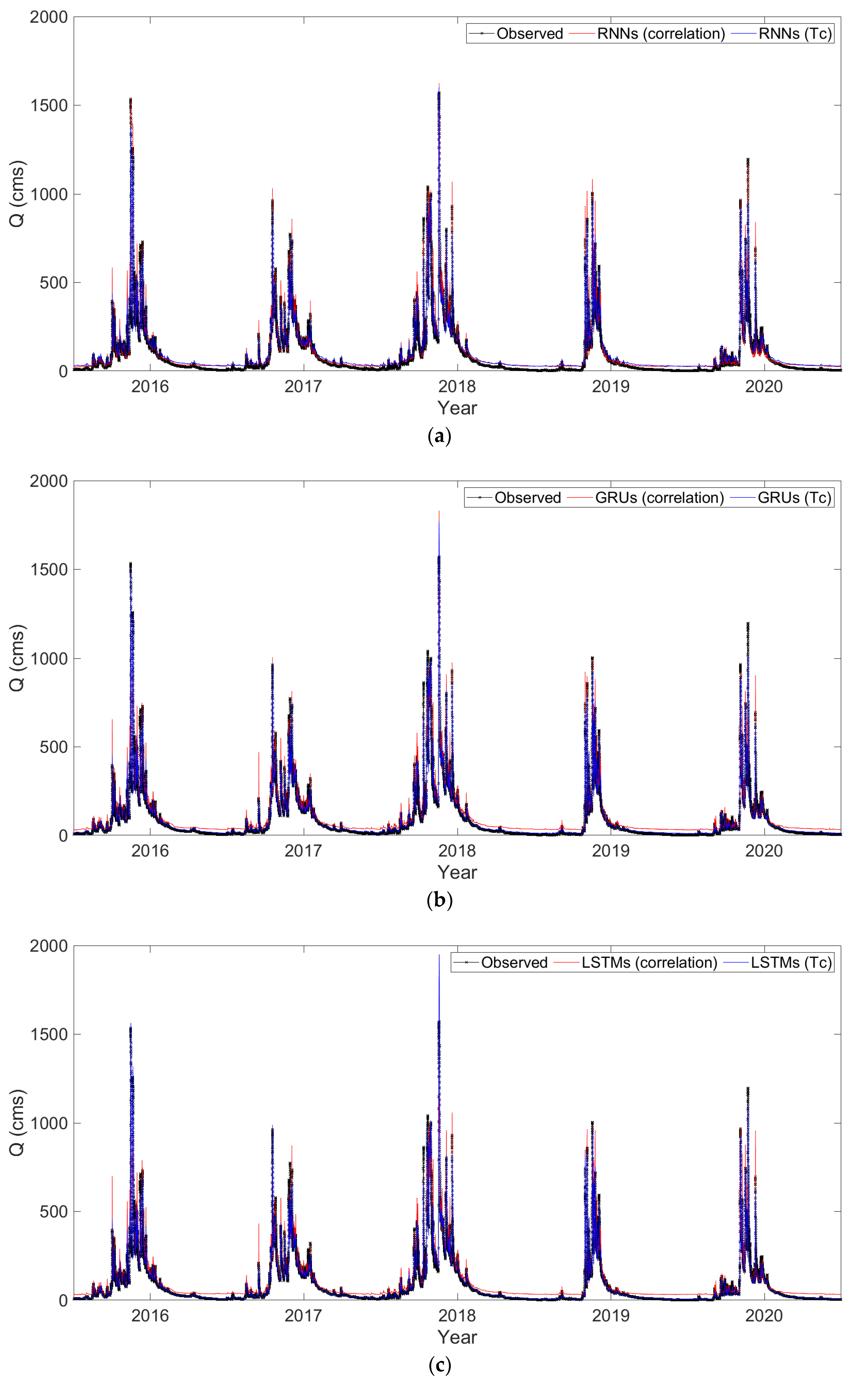
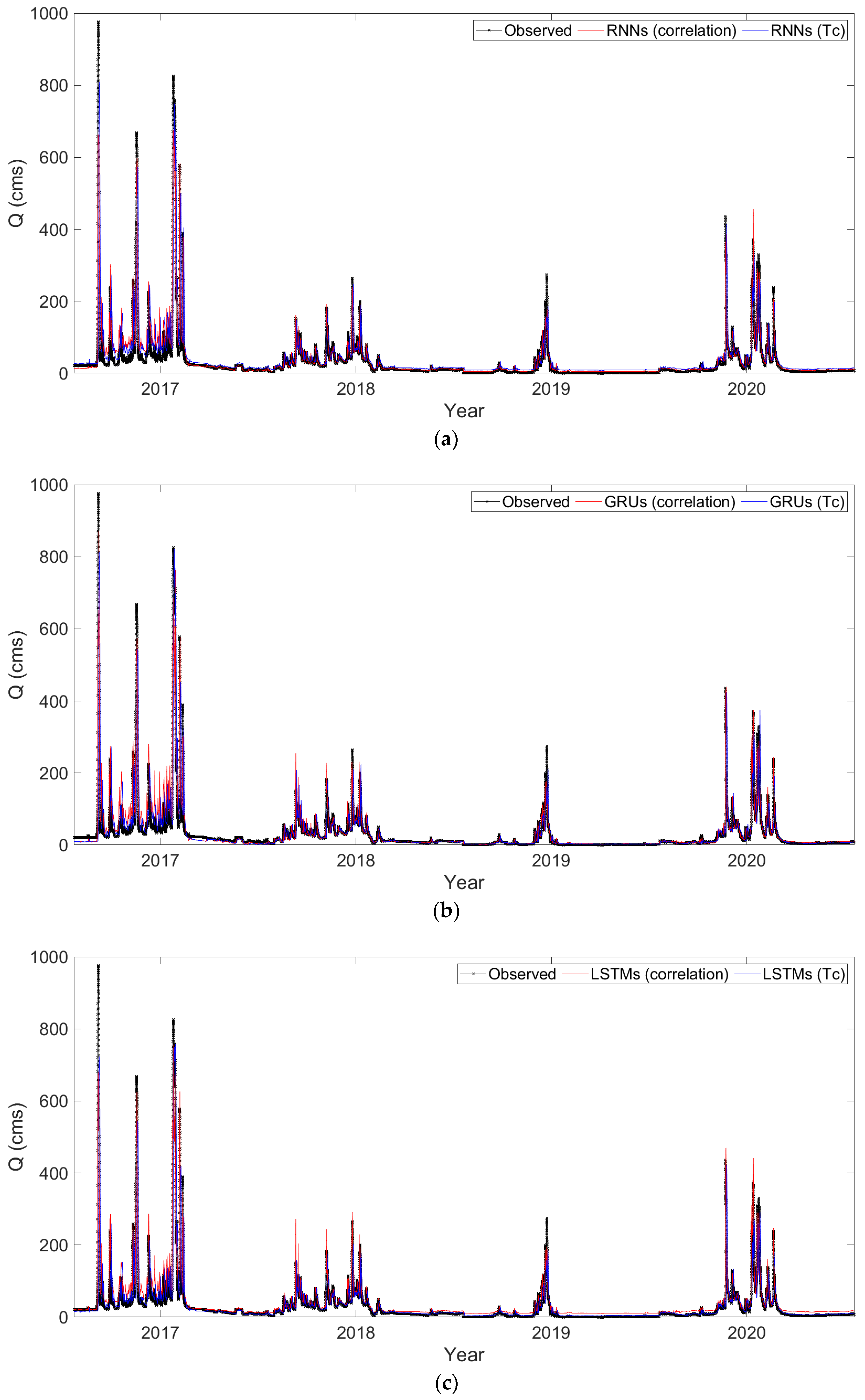
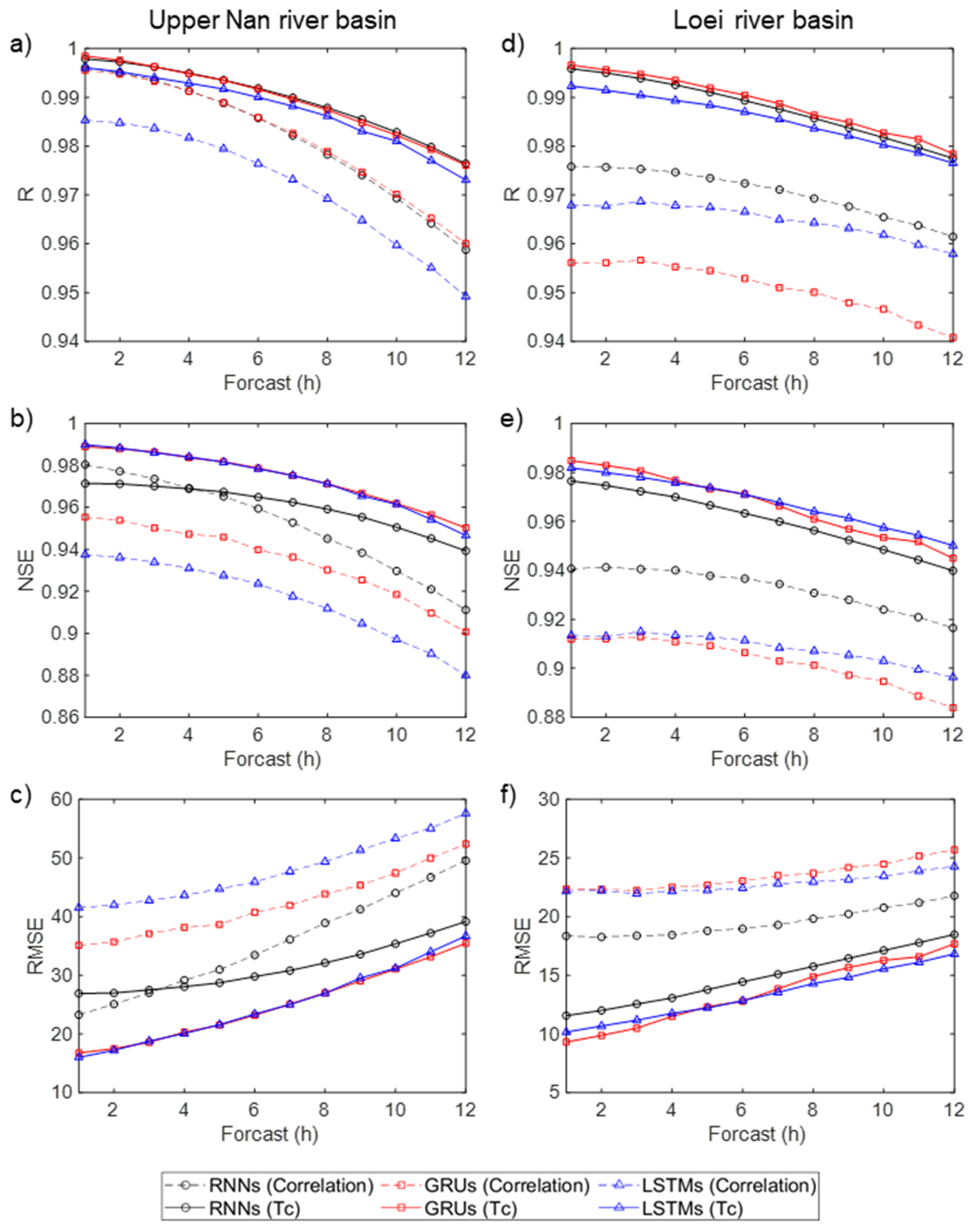
Thorough experiments were conducted with diverse choices of feature representations and network architectures. Three deep learning network architectures consisting of RNNs, GRUs, and LSTMs were compared in this work. These models were carefully fine-tuned to achieve desirable performance. A comparison between observed values and predicted values based on diverse models is provided in Figure 5 and Figure 6 for the Upper Nan and the Loei river basins, respectively. According to these results, all model combinations overestimated the true discharge data. This phenomenon is preferable for precautionary measures with respect to the flood warning system. However, too extreme errors could lead to a false positive warning, which should also be avoided. Among feature representation techniques, utilizing the TC concept yielded fewer overestimated errors than the correlation-based features, as observed in more frequent red spikes in Figure 5 and Figure 6. These observations persisted for both the wet season with peaks of discharge values and the dry season, especially in the latter case. To clearly compare two feature representations, Figure 7 illustrates a comparison of R, RMSE, and NSE based on the correlation-based approach (Case 1) and the TC concept method (Case 2). Results for all 12-step predictions for the Upper Nan (left) and Loei (right) river basins are reported.
According to these results, observed errors regardless of feature representation methods or utilized models were relatively small at the first prediction point. Then, they gradually increased with longer prediction periods and reached the most inferior performance at the 12th farthest point. Using the TC concept in Case 2 generally performed better than the correlation-based approach. These trends were consistent for both the Upper Nan and the Loei river basins as observed in Figure 5 and Figure 6. Incorporating the TC concept based on the time parameter of catchment response was able to identify the accurate required time for the mass of the water to travel from the catchment boundary to the destination station where we aimed to predict. With the use of the NRCS velocity method, the travel time of channel flow from the boundary was considered in Case 2, which exhibited high performance in discharge predictions.
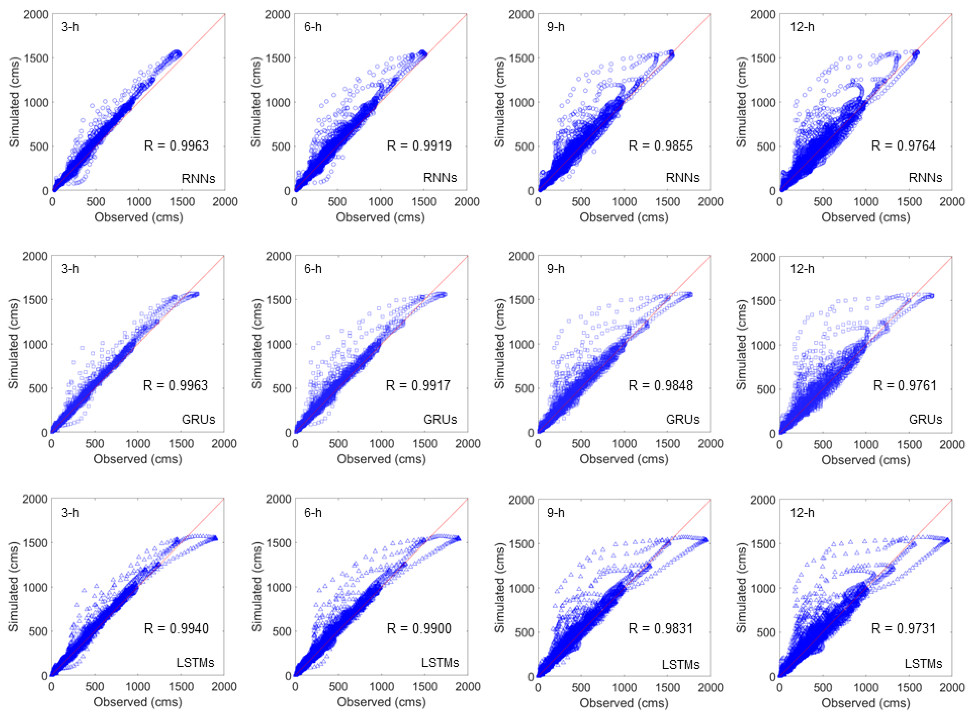
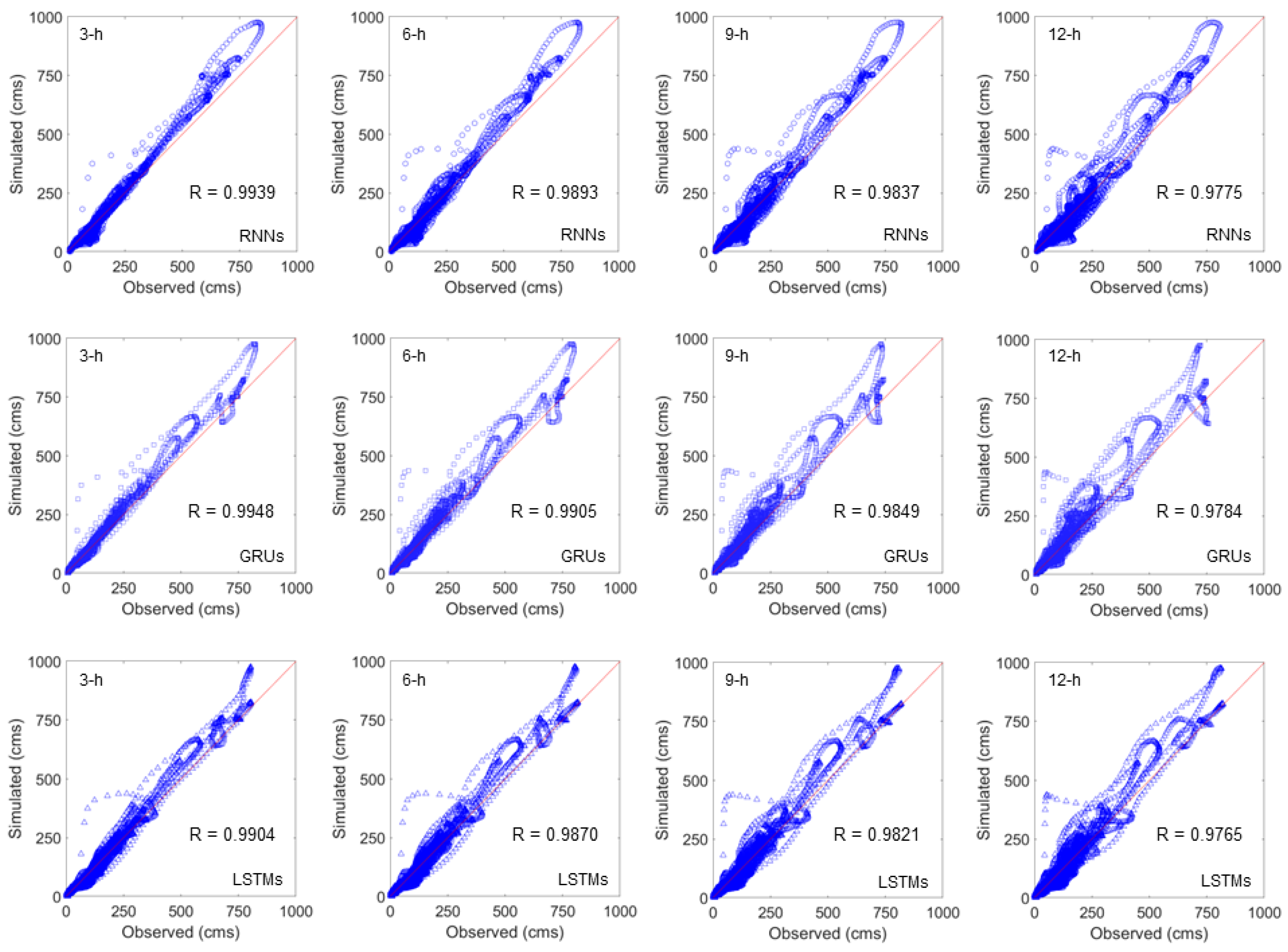
To further evaluate and compare diverse models, we constructed scatter plots between true discharge data and the predicted ones based on the test set. We also considered multiple prediction steps to identify appropriate use cases in real-world applications. Figure 8 depicts scatter plots for the TC feature representation, i.e., Case 2 from RNNs, GRUs, and LSTMs evaluated at 3-h, 6-h, 9-h, and 12-h prediction points for the Upper Nan basin. Similar plots for the Loei basin were constructed, as shown in Figure 9.
Even though RNNs were inferior compared to their two variants based on NSE and RMSE reported in Figure 7, there is no obvious conclusion for R according to Figure 8 and Figure 9. All model networks provided similar results, having high R values with slight variations. The errors were limited at small values and grew substantially for larger discharge data. For the Upper Nan River basin, GRUs yielded slightly better performance with a smaller number of points deviated from the diagonal line, as shown in Figure 8. In terms of deviation directions, all models generally overestimated the true discharge values with small variants at high discharge values of GRUs and LSTMs. Similarly, GRUs and LSTMs provided preferable performance with relatively small RMSE and high NSE. LSTMs are relatively larger and more complicated, which typically work better with large datasets compared to GRUs. With smaller data, LSTMs potentially overfit the training data and fail to generalize with out-of-sample data in the test set. According to our experiment, results among these models were relatively so similar that no obvious conclusion could be made.
Compared with previous studies, we incorporated the TC concept which relied on hydrology domain knowledge, to improve the model performance. Two studied areas of the Upper Nan and the Loei river basins in Thailand were used. This study provided a potential framework for discharge prediction as a universal precautionary measure. Additional steps were required when applying to different datasets. The same networks of RNNs, GRUs, and LSTMS were employed, but computing feature representations and fine-tuning the models were performed separately. Due to the limitation of discharge data availability, the annual rating curve was used to derive the relationship between water level and discharge in this work. Errors were observed from experimented models, especially with longer prediction periods, which should be improved further.
Our future work includes applying additional techniques with more complicated networks to enhance the accuracy of the model. Also, experimenting with the proposed pipeline on additional datasets could confirm observations obtained from our analysis. Rainfall is also an important feature for flood forecasting; however, hourly rainfall data in our study area contains significant missing values. Including rainfall data as input, variables could be further explored in our future work when the data becomes available.
4. Conclusions
In this study, deep learning models were employed to perform a multi-step prediction of the river discharge data. Two study areas of the Upper Nan and the Loei river basins in Thailand were included as our case studies. The correlation-based method was initially used as a feature representation baseline. We further enhanced the feature representations with the Tc concept relying on the hydrograph knowledge. Typical RNNs coupled with more advanced networks like GRUs and LSTMs were experimented with. These models provided similar results with slight variations whereas complicated models, GRUs, and LSTMs provided superior performance for both study areas. Incorporating the TC concept provided more desirable performance regardless of the implemented networks. Further experiments on additional datasets could confirm the results and observations of the analysis. With the current data limitation issue, some insightful input parameters, which potentially enhance the model performance, were excluded.
Author Contributions
Conceptualization, W.T. and P.W.; methodology, W.T.; software, W.S. and P.W.; validation, P.W.; formal analysis, W.S.; investigation, W.T.; data curation, W.T. and W.S.; writing—original draft preparation, W.T. and P.W.; writing—review and editing, P.W.; visualization, W.S.; supervision, W.T. and P.W.; project administration, W.T. All authors have read and agreed to the published version of the manuscript.
Funding
This research was funded by Kasetsart University Research and Development Institute under the grant number FF(KU)25.64.
Institutional Review Board Statement
Not applicable.
Informed Consent Statement
No applicable.
Data Availability Statement
Data available on request due to restrictions, e.g., privacy.
Acknowledgments
This research was supported by Kasetsart University Research and Development Institute under the “FF(KU)25.64” project (to P.W. authors).
Conflicts of Interest
The authors declare no conflict of interest.
References
- Noymanee, J.; Theeramunkong, T. Flood Forecasting with Machine Learning Technique on Hydrological Modeling. Procedia Comput. Sci. 2019, 156, 377–386. [Google Scholar] [CrossRef]
- Cloke, H.L.; Pappenberger, F. Ensemble flood forecasting: A review. J. Hydrol. 2009, 375, 613–626. [Google Scholar] [CrossRef]
- Damle, C.; Yalcin, A. Flood prediction using time series data mining. J. Hydrol. 2007, 333, 305–316. [Google Scholar] [CrossRef]
- Chang, F.J.; Hsu, K.; Chang, L.C. Flood Forecasting Using Machine Learning Methods; MDPI: Basel, Switzerland, 2019; p. 364. [Google Scholar]
- Yaseen, Z.M.; El-Shafie, A.; Jaafar, O.; Afan, H.A.; Sayl, K.N. Artificial intelligence based models for stream-flow forecasting: 2000–2015. J. Hydrol. 2015, 530, 829–844. [Google Scholar] [CrossRef]
- Mosavi, A.; Ozturk, P.; Chau, K.-w. Flood Prediction Using Machine Learning Models: Literature Review. Water 2018, 10, 1536. [Google Scholar] [CrossRef]
- Puttinaovarat, S.; Horkaew, P. Flood Forecasting System Based on Integrated Big and Crowdsource Data by Using Machine Learning Techniques. IEEE Access 2020, 8, 5885–5905. [Google Scholar] [CrossRef]
- Wu, W.; Emerton, R.; Duan, Q.; Wood, A.W.; Wetterhall, F.; Robertson, D.E. Ensemble flood forecasting: Current status and future opportunities. WIREs Water 2020, 7, e1432. [Google Scholar] [CrossRef]
- Ghorpade, P.; Gadge, A.; Lende, A.; Chordiya, H.; Gosavi, G.; Mishra, A.; Hooli, B.; Ingle, Y.S.; Shaikh, N. Flood Forecasting Using Machine Learning: A Review. In Proceedings of the 2021 8th International Conference on Smart Computing and Communications, Kochi, Kerala, India, 1–3 July 2021. [Google Scholar]
- Nguyen, D.T.; Chen, S.-T. Real-Time Probabilistic Flood Forecasting Using Multiple Machine Learning Methods. Water 2020, 12, 787. [Google Scholar] [CrossRef]
- Meshram, S.G.; Meshram, C.; Santos, C.A.G.; Benzougagh, B.; Khedher, K.M. Streamflow Prediction Based on Artificial Intelligence Techniques. Iran. J. Sci. Technol.-Trans. Civ. Eng. 2021, 46, 2393–2403. [Google Scholar] [CrossRef]
- Tongal, H.; Booij, M.J. Simulation and forecasting of streamflows using machine learning models coupled with base flow separation. J. Hydrol. 2018, 564, 266–282. [Google Scholar] [CrossRef]
- Parisouj, P.; Mohebzadeh, H.; Lee, T. Employing Machine Learning Algorithms for Streamflow Prediction: A Case Study of Four River Basins with Different Climatic Zones in the United States. Water Resour. Manag. 2020, 34, 4113–4131. [Google Scholar] [CrossRef]
- Rezaie-Balf, M.; Fani Nowbandegani, S.; Samadi, S.Z.; Fallah, H.; Alaghmand, S. An Ensemble Decomposition-Based Artificial Intelligence Approach for Daily Streamflow Prediction. Water 2019, 11, 709. [Google Scholar] [CrossRef]
- Chen, P.A.; Chang, L.C.; Chang, F.J. Reinforced recurrent neural networks for multi-step-ahead flood forecasts. J. Hydrol. 2013, 497, 71–79. [Google Scholar] [CrossRef]
- Chang, F.J.; Chen, P.A.; Lu, Y.R.; Huang, E.; Chang, K.Y. Real-time multi-step-ahead water level forecasting by recurrent neural networks for urban flood control. J. Hydrol. 2014, 517, 836–846. [Google Scholar] [CrossRef]
- Song, T.; Ding, W.; Wu, J.; Liu, H.; Zhou, H.; Chu, J. Flash Flood Forecasting Based on Long Short-Term Memory Networks. Water 2019, 12, 109. [Google Scholar] [CrossRef]
- Le, X.H.; Ho, H.V.; Lee, G.; Jung, S. Application of Long Short-Term Memory (LSTM) Neural Network for Flood Forecasting. Water 2019, 11, 1387. [Google Scholar] [CrossRef]
- Liu, M.; Huang, Y.; Li, Z.; Tong, B.; Liu, Z.; Sun, M.; Jiang, F.; Zhang, H. The Applicability of LSTM-KNN Model for Real-Time Flood Forecasting in Different Climate Zones in China. Water 2020, 12, 440. [Google Scholar] [CrossRef]
- Kao, I.F.; Zhou, Y.; Chang, L.C.; Chang, F.J. Exploring a Long Short-Term Memory based Encoder-Decoder framework for multi-step-ahead flood forecasting. J. Hydrol. 2020, 583, 124631. [Google Scholar] [CrossRef]
- Gude, V.; Corns, S.; Long, S. Flood Prediction and Uncertainty Estimation Using Deep Learning. Water 2020, 12, 884. [Google Scholar] [CrossRef]
- Apaydin, H.; Feizi, H.; Sattari, M.T.; Colak, M.S.; Shamshirband, S.; Chau, K.W. Comparative Analysis of Recurrent Neural Network Architectures for Reservoir Inflow Forecasting. Water 2020, 12, 1500. [Google Scholar] [CrossRef]
- U.S. Department of Agriculture Natural Resources Conservation Service (USDA-NRCS). Time of concentration. In National Engineering Handbook (NEH); U.S. Department of Agriculture Natural Resources Conservation Service (USDA-NRCS): Washington, DC, USA, 2010; p. 29. [Google Scholar]
- Gericke, O.J.; Smithers, J.C. Review of methods used to estimate catchment response time for the purpose of peak discharge estimation. Hydrol. Sci. J. 2014, 59, 1935–1971. [Google Scholar] [CrossRef]
- Kirpich, Z.P. Time of Concentration of Small Agricultural Watersheds. Civ. Eng. 1940, 10, 362. [Google Scholar]
- Kerby, W.S. Time of Concentration for Overland Flow. Civ. Eng. 1959, 29, 174. [Google Scholar]
- Morgali, J.R.; Linsley, R.K. Computer simulation of overland flow. J. Hydraul. Div. ASCE 1965, 90, 81–100. [Google Scholar] [CrossRef]
- Federal Aviation Administration (FAA). Circular on Airport Drainage; U.S. Department of Transportation: Washington, DC, USA, 1970; p. 80.
- US Bureau of Reclamation (USBR). Design of Small Dams; US Department of the Interior, Bureau of Reclamation: Washington, DC, USA, 1973; p. 860.
- Watt, W.E.; Chow, K.C.A. A general expression for basin lag time. Can. J. Civ. Eng. 1985, 12, 294–300. [Google Scholar] [CrossRef]
- Seybert, T.A. Stormwater Management for Land Development; John Wiley & Sons, Inc.: Hoboken, NJ, USA, 2006; p. 372. [Google Scholar]
- Aziz, K.; Haque, M.M.; Rahman, A.; Shamseldin, A.Y.; Shoaib, M. Flood estimation in ungauged catchments: Application of artificial intelligence based methods for Eastern Australia. Stoch. Environ. Res. Risk Assess. 2017, 31, 1499–1514. [Google Scholar] [CrossRef]
- Hazzab, A.; Seddini, A.; Ghenaim, A.; Korichi, K. Hydraulic flood routing in an ephemeral channel: Wadi Mekerra, Algeria. Model. Earth Syst. Environ. 2016, 2, 1–12. [Google Scholar]
- Fang, X.; Thompson, D.B.; Cleveland, T.G.; Pradhan, P. Variations of Time of ConcentrationEstimates Using NRCS Velocity Method. J. Irrig. Drain. Eng. 2007, 133, 314–322. [Google Scholar] [CrossRef]
- Perdikaris, J.; Gharabaghi, B.; Rudra, R. Reference Time of Concentration Estimation for UngaugedCatchments. Earth Sci. Res. J. 2018, 7, 58–73. [Google Scholar] [CrossRef]
- Lipton, Z.C.; Berkowitz, J.; Elkan, C. A Critical Review of Recurrent Neural Networks for Sequence Learning. arXiv 2015, arXiv:1506.00019. [Google Scholar]
- Chung, J.; Gulcehre, C.; Cho, K.; Bengio, Y. Empirical Evaluation of Gated Recurrent Neural Networks on Sequence Modeling. arXiv 2014, arXiv:1412.3555. [Google Scholar]
- Rahimzad, M.; Moghaddam Nia, A.; Zolfonoon, H.; Soltani, J.; Danandeh Mehr, A.; Kwon, H.-H. Performance Comparison of an LSTM-based Deep Learning Model versus Conventional Machine Learning Algorithms for Streamflow Forecasting. Water Resour. Manag. 2021, 35, 4167–4187. [Google Scholar] [CrossRef]
- Krause, P.; Boyle, D.P.; Bäse, F. Comparison of different efficiency criteria for hydrological model assessment. Adv. Geosci. 2005, 5, 89–97. [Google Scholar] [CrossRef]
- Kan, G.; Liang, K.; Yu, H.; Sun, B.; Ding, L.; Li, J.; He, X.; Shen, C. Hybrid machine learning hydrological model for flood forecast purpose. Open Geosci. 2020, 12, 813–820. [Google Scholar] [CrossRef]
Figure 1.
Study area equipped with the stream gauges of the Upper Nan River basin (left) and the Loei river basin (right).
Figure 1.
Study area equipped with the stream gauges of the Upper Nan River basin (left) and the Loei river basin (right).

Figure 2.
A flow process chart.

Figure 3.
Discharge data collected from stations located in the Upper Nan river basin.

Figure 4.
Discharge data collected from stations located in the Loei river basin.

Figure 5.
The comparison of observed discharge and 12-h predicted discharge using deep learning model for the Upper Nan River basin (a) RNNs (b) GRUs and (c) LSTMs.
Figure 5.
The comparison of observed discharge and 12-h predicted discharge using deep learning model for the Upper Nan River basin (a) RNNs (b) GRUs and (c) LSTMs.

Figure 6.
The comparison of observed discharge and 12-h predicted discharge using deep learning model for the Leoi River basin (a) RNNs (b) GRUs and (c) LSTMs.
Figure 6.
The comparison of observed discharge and 12-h predicted discharge using deep learning model for the Leoi River basin (a) RNNs (b) GRUs and (c) LSTMs.

Figure 7.
A comparison of R, RMSE and NSE for correlation-based and TC-based features using deep learning models for the Upper Nan (left) and Loei (right) river basins. (a) R on the Upper Nan river basin; (b) NSE on the Upper Nan river basin; (c) RMSE on the Upper Nan river basin; (d) R on the Loei river basin; (e) NSE on the Loei river basin; (f) RMSE on the Loei river basin.

Figure 8.
Scatter plots between observed data and the simulated prediction at 3-h, 6-h, 9-h, and 12-h of RNNs, GRUs, and LSTMs using the TC feature representations for the Upper Nan river basin.
Figure 8.
Scatter plots between observed data and the simulated prediction at 3-h, 6-h, 9-h, and 12-h of RNNs, GRUs, and LSTMs using the TC feature representations for the Upper Nan river basin.

Figure 9.
Scatter plots between observed data and the simulated prediction at 3-h, 6-h, 9-h, and 12-h of RNNs, GRUs, and LSTMs using the TC feature representations for the Loei river basin.
Figure 9.
Scatter plots between observed data and the simulated prediction at 3-h, 6-h, 9-h, and 12-h of RNNs, GRUs, and LSTMs using the TC feature representations for the Loei river basin.

Publisher’s Note: MDPI stays neutral with regard to jurisdictional claims in published maps and institutional affiliations. |
© 2022 by the authors. Licensee MDPI, Basel, Switzerland. This article is an open access article distributed under the terms and conditions of the Creative Commons Attribution (CC BY) license (https://creativecommons.org/licenses/by/4.0/).
Share and Cite
MDPI and ACS Style
Thaisiam, W.; Saelo, W.; Wongchaisuwat, P. Enhancing a Multi-Step Discharge Prediction with Deep Learning and a Response Time Parameter. Water 2022, 14, 2898. https://doi.org/10.3390/w14182898
AMA Style
Thaisiam W, Saelo W, Wongchaisuwat P. Enhancing a Multi-Step Discharge Prediction with Deep Learning and a Response Time Parameter. Water. 2022; 14(18):2898. https://doi.org/10.3390/w14182898
Chicago/Turabian StyleThaisiam, Wandee, Warintra Saelo, and Papis Wongchaisuwat. 2022. "Enhancing a Multi-Step Discharge Prediction with Deep Learning and a Response Time Parameter" Water 14, no. 18: 2898. https://doi.org/10.3390/w14182898
Note that from the first issue of 2016, this journal uses article numbers instead of page numbers. See further details here.