

Hydraulic Transient Simulation of Pipeline-Open Channel Coupling Systems and Its Applications in Hydropower Stations
1
State Key Laboratory of Water Resources and Hydropower Engineering Science, Wuhan University, Wuhan 430072, China
2
School of Civil, Environmental & Mining Engineering, The University of Adelaide, Adelaide, SA 5005, Australia
3
Power China Kunming Engineering Corporation Limited, Kunming 650051, China
*
Author to whom correspondence should be addressed.
Water 2022, 14(18), 2897; https://doi.org/10.3390/w14182897
Submission received: 11 August 2022
/
Revised: 5 September 2022
/
Accepted: 7 September 2022
/
Published: 16 September 2022
(This article belongs to the Special Issue About an Important Phenomenon—Water Hammer)
Abstract
:Hydraulic systems may involve both pipelines and open channels, which challenges the hydraulic transient analysis. In this paper, a method of characteristics (MOC)-finite volume method (FVM) coupling method has been developed with the pipeline modelled using the MOC and the open channel modelled using the FVM. The coupling boundaries between these two simulation regions are developed based on Riemann invariants. The simulated parameters can be transmitted from the MOC region to the FVM region and in the reverse direction through the coupling boundaries. Validation of the method is conducted on a simple tank-pipe system by comparing the simulated result using 3D computational fluid dynamics (CFD) analysis. The new method is then applied to a prototype hydropower station with a sand basin located between the upstream reservoir and the turbines. The sand basin is modelled as an open channel coupled with the pipes in the system. The transient processes are also simulated by modelling the sand basin as a surge tank. The comparison with the results by the MOC-FVM coupling method shows the new coupling method can provide more reliable and accurate results. This is because the flow velocity in the horizontal direction in the sand basin is considered in the coupling method but neglected when the sand basin is modelled as a surge tank in the MOC.
1. Introduction
Hydraulic transients occur regularly in hydraulic systems conveying fluids, such as water distribution systems, pumping stations [1], subsea pipelines [2] and hydropower stations [3]. They can cause large pressure surges which may damage the pipe assets and lead to operation instabilities when a control system is in operation together with the hydraulic system. Therefore, conducting hydraulic transient simulation is important to facilitate the design of hydraulic systems [4].
Traditional methods to simulate hydraulic transient events include the method of characteristics (MOC) [5,6], the finite-difference method, the finite volume method and frequency domain methods (e.g., transfer matrix method [7]). The MOC gradually becomes the most popular in real engineering practices. The transient simulation software programs to solve engineering problems are mostly based on MOC with some exceptions (e.g., [8]). One of the reasons for its popularity is its ability to consider complicated phenomena, such as the fluid-structure interaction [9], pipe wall viscoelasticity [10] and unsteady friction [11]. Another reason is its simplicity to be integrated with the modelling of other subsystems in a complicated system. For example, the transient simulation of a hydropower station involves the modelling of the turbines, pressure surge control elements (e.g., surge tanks), the control system (to control the operation of guide vanes) and sometimes the electrical system [3].
In engineering practice, some pressurized pipe flow in these hydraulic systems may be coupled with free-surface open channel flow. For example, a division canal may be used to deliver water to the inlet of a pump station. Another example used in some hydropower stations is the sand basin which can also suppress the pressure surge during the transient events. Traditional methods to simulate free surface open channel flow include the finite element method (FEM), the finite-difference method (FDM) and the finite volume method (FVM) [12]. Since the FVM possesses high efficiency and accuracy, modelling flexibility and clear physical meaning [13], the FVM is adopted in this study for open channel flow simulation.
One of the common measures in practice for simulating pipeline-open channel coupling systems is to neglect the effects of the open channel on the pressure response of the entire system. This is because the magnitude of the wave oscillation in the open channel is relatively small compared with the pressure surge in the pressurized pipe. Such measures are acceptable when the open channel is relatively short and only the pressure magnitude in the pipe is of interest. However, such approximation may reduce the accuracy of the simulation especially when the channel plays an important role in the transient response (e.g., the channel is located between two pressurized pipes). Another solution to such issues is the 1D-3D coupling simulation [14,15,16,17] with pipelines modelled using 1D MOC and other parts modelled with a 3D CFD method. For example, the ANSYS-fluent package can be used for 3D CFD simulation coupling with 1D MOC simulation in hydropower stations and pump stations. This method shows its advantages when the 3D region possesses a complicated geometry that is difficult to simplify to a 1D or 2D model, such as pump turbines in [16]. However, this method requires high computational resources, which conflicts with the requirement of fast computation and sometimes near-real time simulation for many engineering cases (e.g., hydropower stations, pump stations) involving open channels. The geometries of the open channels in these cases are relatively simple, and mostly can be simplified into a 1D model.
To address the engineering issue described above, this paper proposed a coupling method to simulate such coupling systems. The 1D MOC method is still used to model the pipes in the complicated system, the FVM is used to simulate the open channel flow in the system, and the coupling boundary is developed based on Riemann invariants. Such coupling method has been integrated into the comprehensive transient modelling software program TOPSYS which has been developed by the transient research group at Wuhan university [3,18] and validated through both model testing [19] and prototype testing [20]. This enables the simulation of complicated hydropower systems with considering the effects of the open channel components in the system.
The structure of the paper is as follows: Following the literature review in the introduction, the next section illustrates the methodologies to develop the coupling transient simulation. The 1D simulation method is then numerically validated with a 3D CFD case on a simple tank-pipe coupling system. The validated method is then applied to a prototype hydropower station to solve an engineering problem associated with a sand basin. The simulation results by the new method compared with the traditional transient simulation method (MOC) in this hydropower system illustrate the distinctive effects of the sand basin on both the magnitude and the period of the pressure surge wave as well as on the operation stability of the hydropower system.
2. Mathematical Model and Verifications
2.1. Transient Modelling of Pipeline Flow
The continuity and momentum equations of the pipeline transient flows are given as follows [21]:
in which is the piezometric head; is the discharge; is the distance; is the time; is the wave speed of the transient waves; is the gravitational acceleration; is the Darcy-Weisbach friction factor; is the pipe diameter; and is the cross-sectional area.
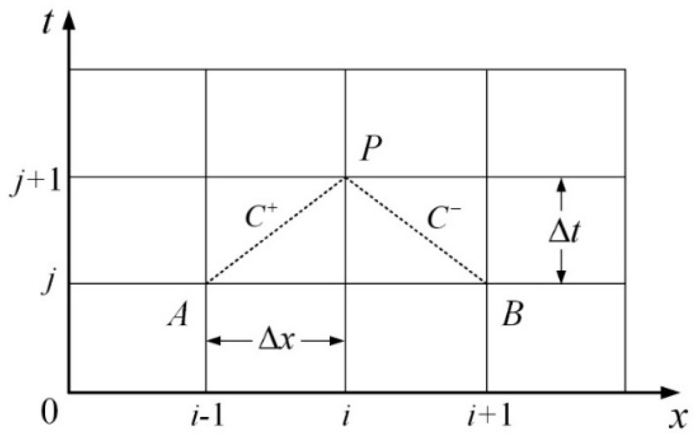
The method of characteristics is widely used to solve Equations (1) and (2) and is briefly introduced below. The partial differential equations can be transformed into ordinary differential equations by:
which are valid along with the positive () and negative () characteristic lines, as shown in Figure 1. The subscripts i − 1, i and i + 1 represent the space steps. By rearranging Equations (3) and (4), the following compatibility equations can be obtained:
where ; ; ; . Details of the method can be found in [21].
According to the space-time plane as shown in Figure 1, the parameters and at time step j + 1 can be calculated by using Equations (5) and (6) if , , and at time step j have already been obtained from the calculation in the time step j − 1 or are already known from the steady state condition.
Apart from the MOC, the Preissmann four-point finite-difference method (FDM) can be also used to solve Equations (1) and (2). By using a forward scanning method [21], a linear relationship between the flow rate and the pressure head at each grid node can be obtained as:
where and are two terms that are related to the boundary conditions, the piezometric head and the discharge at node i and at the time step j. Details of the method can be found in [21].
It can be found from Equations (5)–(7) that a linear relationship between the flow rate and the pressure head can be obtained in both MOC and FDM. Both linear equations can be used to be coupled with the FVM which is used to solve the open channel flow. In the case studies in this paper, the MOC was used to simulate the pipeline flow. But it should be noted that the proposed coupling technique applies to FDM as well.
2.2. Modelling of Open Channel Flow
The continuity and momentum equations of the open channel flow are given as [22,23]
with
in which U is the vector of conserved variables, F is the vector of fluxes and each of its components is a function of the components of U, S is the source term, u is the flow velocity in the x-direction which is along with the channel, h is the water depth, q is the discharge per unit width, z is the bottom elevation of the channel, τ is a parameter on the friction of the channel wall and can be expressed as with representing the Manning coefficient.
In this paper, this non-linear equation group is linearized locally and the fluxes at the grid interfaces are calculated using the Roe–average parameters. The Godunov-type finite volume method (FVM) [22,23] is applied to solve Equation (9). The grids in the FVM are shown in Figure 2, in which the grid node i + 1/2 is defined as the shared node of grid i and grid i + 1, and the subscripts L and R are the vectors on the left side and the right side of a grid node, respectively, and the total number of the grids is N.
Integrating the continuity equation and the momentum equation for the control volume i gives:
By setting and as the averaged values of the control volume i, Equation (10) can be then rewritten as:
with the source term expressed as
in which the superscript k is the number of the time step, and the subscript i is the grid number. It should be noted that i represents the number of the grid node in the MOC and FDM. The symbols and are the duration of the time step and the size of the grid, respectively. The following processes show the procedures to calculate the vectors of fluxes and [22,23].
Equation (8) can be rewritten as:
in which A is the Jacob matrix of the flux function F(U) and can be expressed as:
The linearization of Equation (14) gives:
in which is a constant matrix and can be calculated based on the known UL and UR by
in which . The eigenvalues of are:
and the corresponding right eigenvectors are:
The wave strength, can be obtained using the following equation
with the solutions as:
in which , . The flux and can be then obtained using
2.3. Boundary Condition Based on Riemann Invariants
A general m-dimensional quasi-linear hyperbolic system can be given as [22,23]:
in which is the vector of dependent variables. The corresponding right eigenvector of the wave associated with ith characteristic field with eigenvalue is:
The generalized Riemann invariants are relations that hold for each wave, leading to m-1 ordinary differential equations as:
For the open channel equations, the right eigenvectors are:
Thus, substituting Equation (28) into Equation (27) gives
By taking the relationship
into Equation (30), it gives
which can be rearranged to
The integration of Equation (33) gives
According to Equation (34), the flow velocity and pressure head at the downstream boundary in the FVM region at the time step k+1 can be linked with those at the centre of the last FVM grid in the downstream side at the time step k. The expression is given as:
Similar processes can be conducted on the upstream coupling boundary using Equations (34) and (29). The result can be obtained as
It should be noted that the coupling boundary equations (Equations (35) and (36)) are only applicable to open channels with a subcritical flow which is the case for most engineering applications.
2.4. The Simulation Process
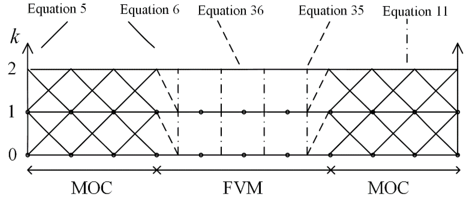
With all the equations listed above, this section gives the processes of the coupling simulation using the grid schematic as shown in Figure 3. To include the coupling boundaries that transmit data from both MOC to FVM and from FVM to MOC, a MOC-FVM-MOC coupling system with 10 grids is used to illustrate the simulation process. The horizontal and vertical coordinates represent the space step and the time step, respectively. The dots on the horizontal coordinate are the grid nodes. In the MOC regions, the solid diagonals represent the calculation process of the C+ (Equation (5)) and C− (Equation (6)) equations and the vertical lines which are superposed on the vertical coordinates mean the boundary conditions that are determined by the system. In the FVM region, the vertical dot-dashed lines represent the calculation process of Equation (11). The dash lines in the leftmost grids in the FVM region represent the coupling boundary of Equation (36) and those in the rightmost grids in the FVM region represent the coupling boundary of Equation (35). Starting from k = 0 with the initial parameters known, the simulation processes are represented by these lines in Figure 3.
3. Numerical Validations
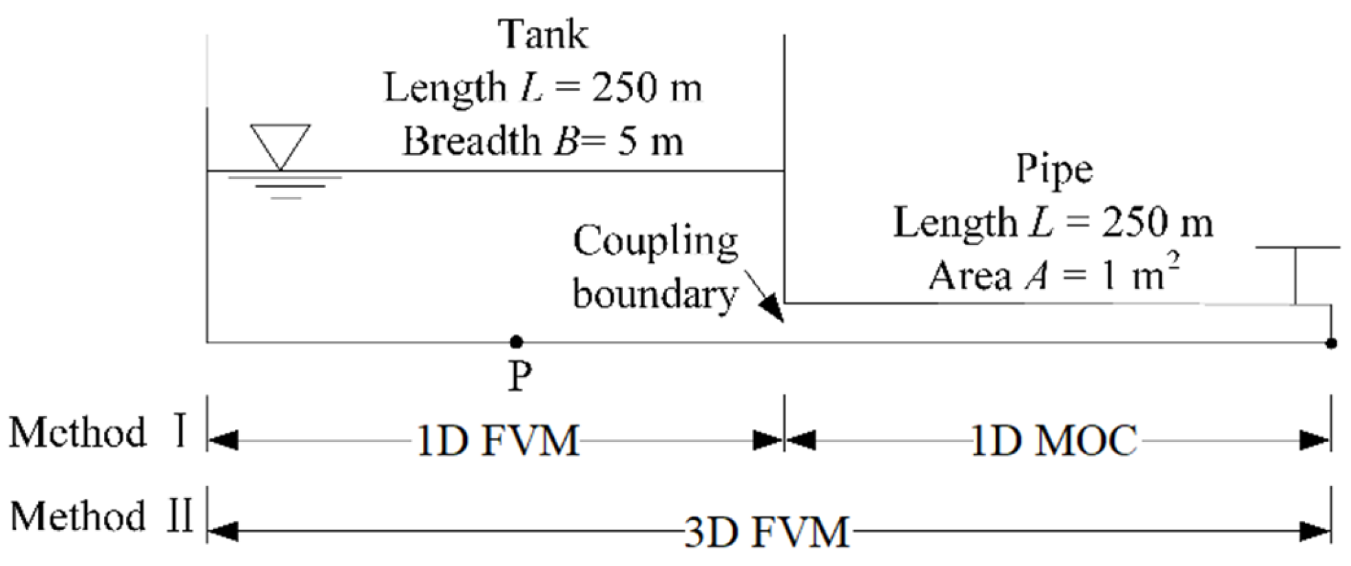
As shown in Figure 4, a tank-pipe system was used to validate the MOC-FVM coupling method. The tank at the upstream side of the pipe is 250 m in length and 5 m in width with an initial water depth of 2 m. The bottom of the tank is horizontal. The pipeline is 250 m in length with the area of the cross-section equal to 1 m2. The wave speed of transient waves in the pipeline is 1000 m/s. The initial flow rate in the pipe is 0 m/s with the valve fully closed at the downstream end of the pipeline. Water is transmitted to the pipeline through the valve and the flow rate increases from 0 m3/s to 2m3/s in 5 s and keeps constant at 2 m3/s after 5 s. The friction losses in the tank and pipeline are neglected in this validation case.
Two methods were applied to simulate this tank-pipe case. The first method (Method I) is the proposed MOC-FVM coupling method. The time step in the simulation is 0.005 s and the spatial step is 5 m for the 1D meshes. The 3D FVM method (Method II) is used to validate the proposed coupling method. In Method II, the whole system including the tank and the pipe is modelled in three dimensions using ANSYS Fluent (3D FVM based simulation). The size of the meshes is 0.2 m and the fluid is assumed as inviscid.
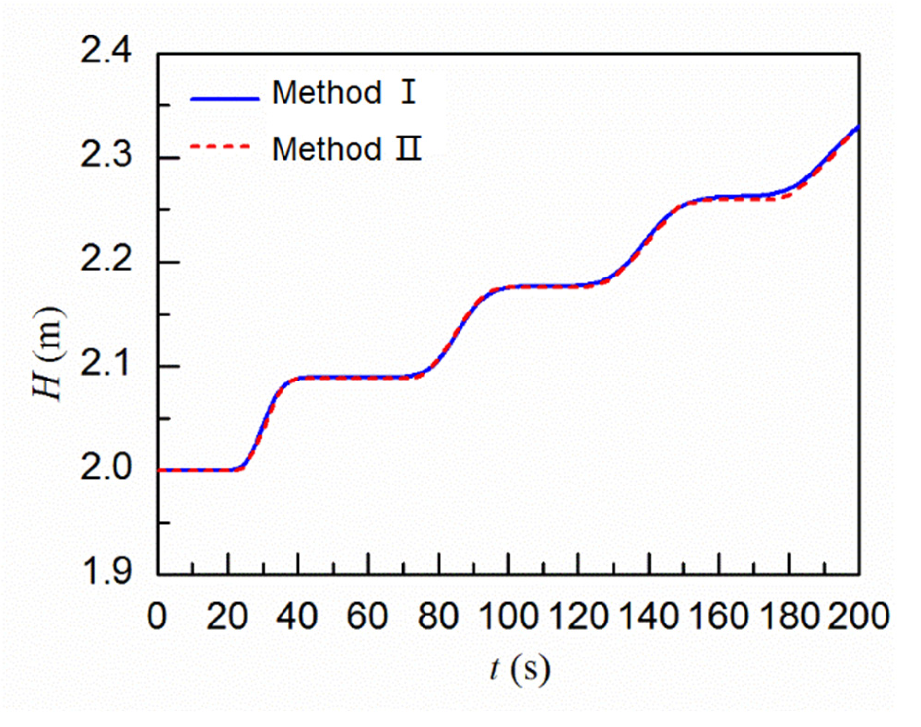
The water depth at position P in Figure 4 is monitored in both simulations. The variations of the water depths from these two simulations are compared in Figure 5, which shows the simulated results are almost identical. The comparison illustrates the proposed MOC-FVM coupling method is able to simulate the unsteady flow for a pipeline-open channel coupling system.
4. Transient Simulation of a Hydropower Station with a Sand Basin
4.1. System Configuration and Modelling
The schematic of the hydropower station is shown in Figure 6. There are three Francis turbines in the station and they share one main penstock on the upstream side. A rectangle open channel is planned to build between the upstream reservoir and the turbines to serve as a sand basin. The length of the sand basin is set as Ls and the width is w. The initial water depth in the sand basin is h. the Manning coefficient in the sand basin is 0.014. The length of the tunnel between the upstream reservoir and the sand basin is L1 and the length of the penstock between the sand basin and the bifurcation is L2. The sum of L1 and L2 is 3370 m and the diameter of the tunnel and penstock are both 8.7 m. The wave speeds of the transient wave in the pipelines are calculated based on the theoretical equation [5] and are around 1100 m/s. The Darcy-Weisbach coefficient is 0.02. Some other basic information about the hydropower station is shown in Table 1.
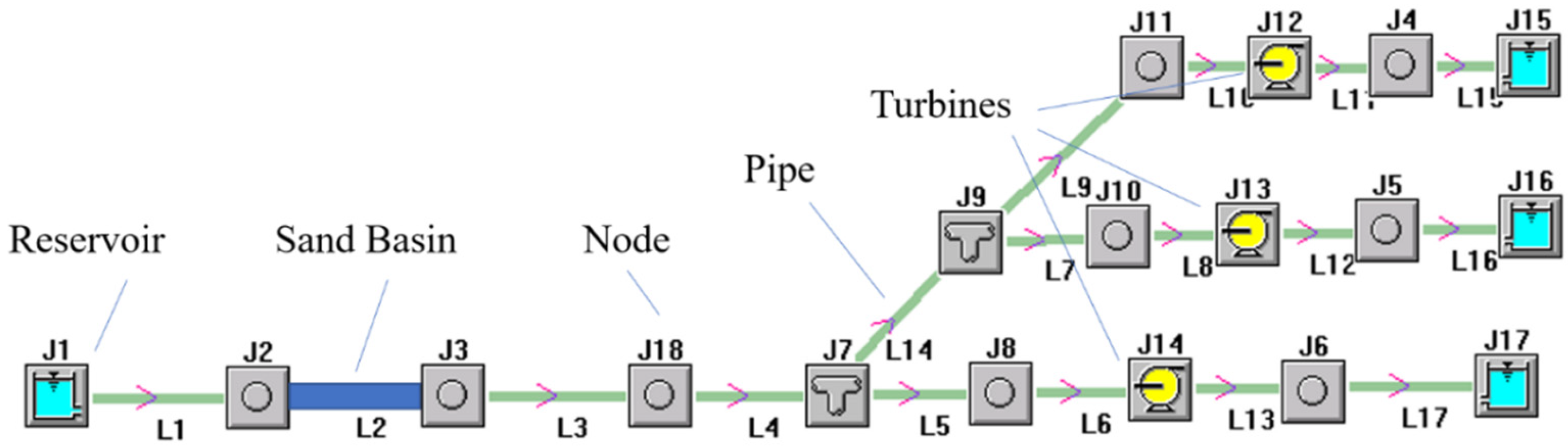
The proposed MOC-FVM method has been integrated into the hydraulic transient simulation program–TOPSYS as shown in Figure 7. The pipe system in the hydropower station is simulated using the proposed MOC-FVM coupling method. The tunnel, penstock, upstream reservoir and branch pipes are simulated using the MOC with the sand basin simulated using the FVM. To simulate the hydraulic transient process of the hydropower station, the turbines and the controller of the servomotor that drives the guide vanes are also modelled with details of the modelling shown in [3]. The characteristic curves are adopted to model the turbines and a PID controller is used to control the movement of the guide vanes.
4.2. Full Load-Rejection
4.2.1. Simulation Results
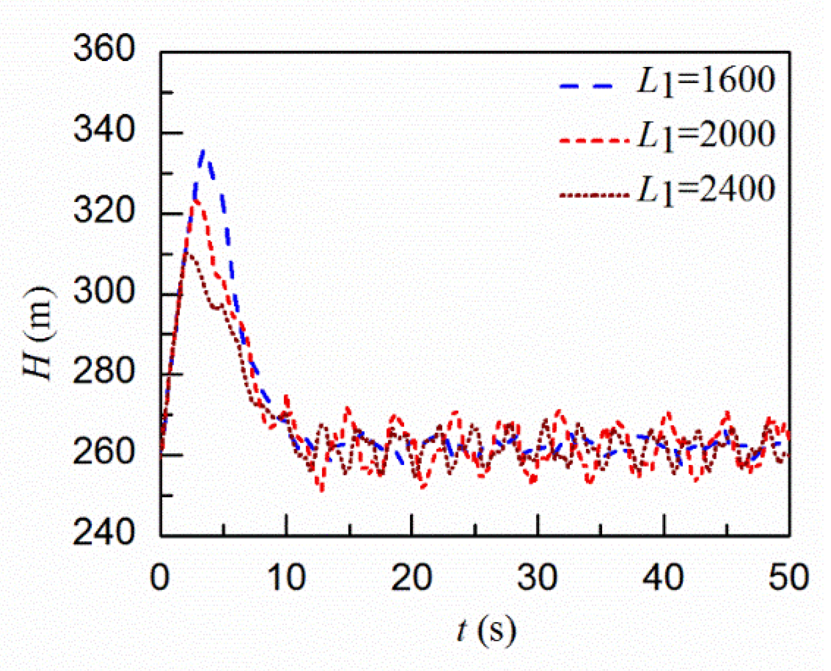
In this case, all the three turbines reject their loads simultaneously. The guide vanes of the turbines are closed linearly within 10 s. The transient waves caused by the closure of the guide vanes will be partially reflected by the sand basin and the reflected waves will be superimposed with the incident waves. The wave reflection and superposition process will be affected by the position of the sand basin. Thus, three scenarios with L1 = 1600 m, 2000 m and 2400 m, respectively, were simulated to illustrate the effects of the position of the sand basin on the transient performance of the hydropower station. The pressure heads at the inlet of the spiral case for these three scenarios were compared in Figure 8, which shows the maximum water hammer pressure decreases when the sand basin gets closer to the turbines. The wave fluctuations after 10 s are the water hammer waves and their periods are associated with the wave traveling time in the penstocks.
Another two scenarios with L1 = 2400 m were conducted by changing the bottom elevation and the width of the sand basin, respectively. The comparison of the pressure heads at the inlet of the spiral case for these two scenarios with the original scenario is shown in Figure 9. The results show that the bottom elevation and width of the basin do not distinctively affect the water hammer pressure. This is because the pressure reaches its maximum shortly (within 5 s) after the load rejection, while the wave oscillation caused by the sand basin has a much large period (as shown in Figure 10).
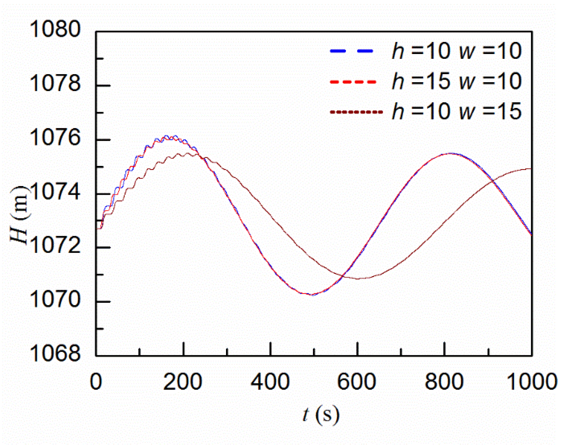
The water level variations at the central point of the tank with L1 = 2400 m are compared in Figure 10 for different sizes of the sand basin. The comparison shows the bottom elevation of the sand basin has a slight effect on the water level fluctuation. The width of the basin, however, affects the water level variation significantly with the period of the oscillation increasing and the magnitude decreasing for a wider basin.
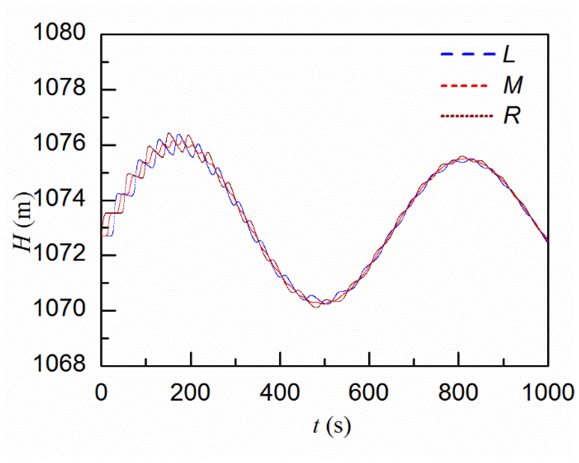
The water levels at different positions (left side L, central point M and right side R) of the sand basin are compared in Figure 11 when L1 = 2400 m, h = 10 m and w = 10 m. The comparison shows the overall trend of the water level oscillations at these three points are the same, but different wave oscillations with a short period are superimposed with the low-frequency oscillation. This is caused by the wave propagating in the horizontal direction along the sand basin during the transient process.
4.2.2. Comparison with the Results by Modelling the Basin Tank as a Surge Tank
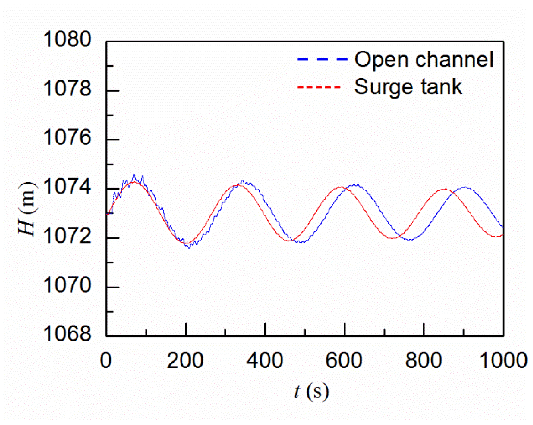
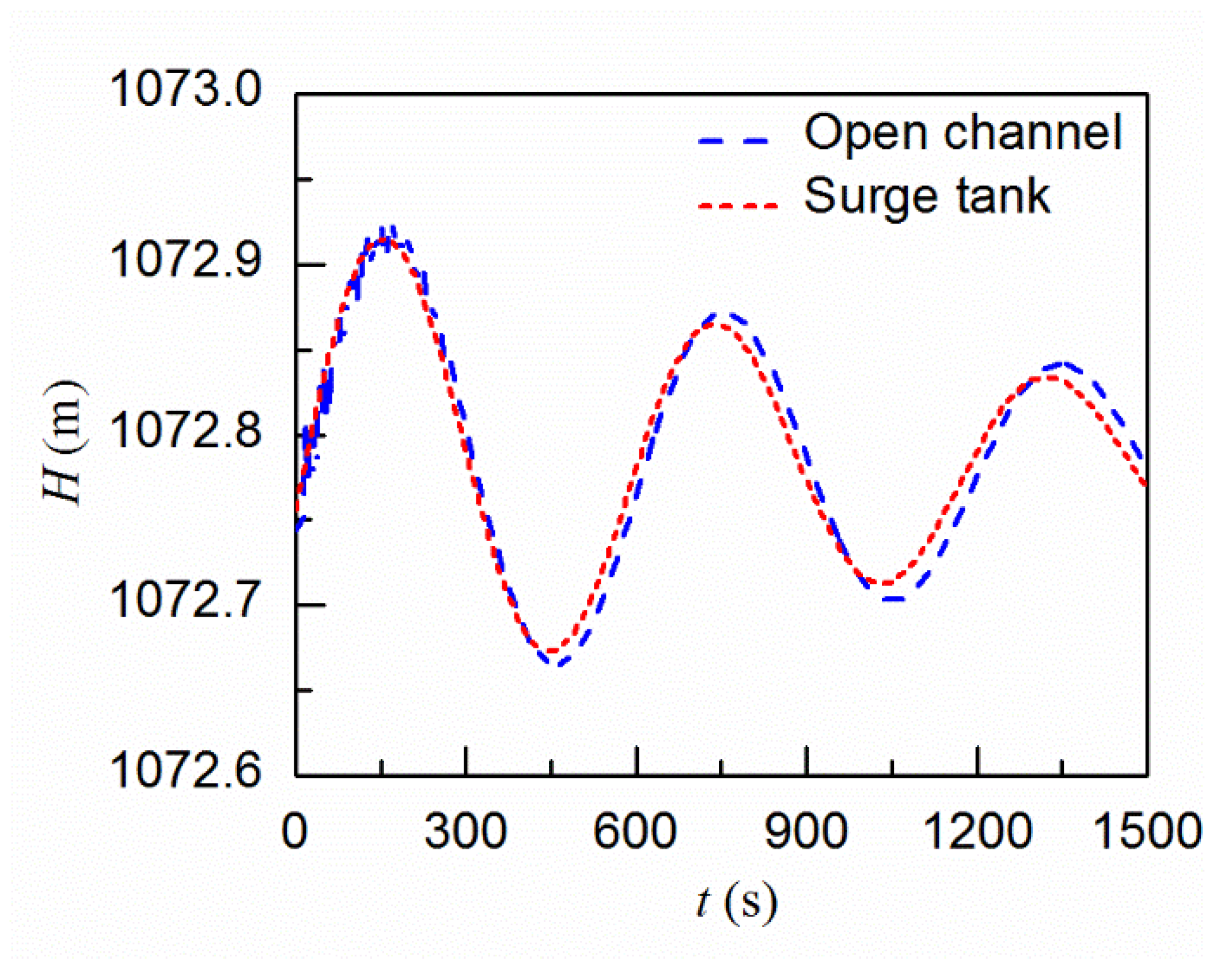
In the previous section, the sand basin is treated as an open channel which is modelled using the FVM. Another modelling method of the sand basin is to simplify it as a surge tank in the hydropower station. With the length of 250 m and width of 10 m for the sand basin, the equivalent area of the surge tank used to model the sand basin is calculated as 2500 m2. The simulated results by treating the sand basin as a surge tank and those by modelling the sand basin as an open channel are compared in Figure 12 and Figure 13. When the sand basin is close to the turbines (L1 = 2400 m), a slight difference can be found in the period and magnitude of the water level fluctuations in the sand basin. A more distinctive difference can be observed when the sand basin is far away from the turbines (L1 = 400 m). Such differences can be ascribed to the fact that the flow velocity and friction in the sand basin along the horizontal direction are neglected in the surge tank modelling but incorporated in the FVM when modelling the sand basin.
4.3. 5% Load-Rejection with Frequency Regulation
4.3.1. Simulation Results
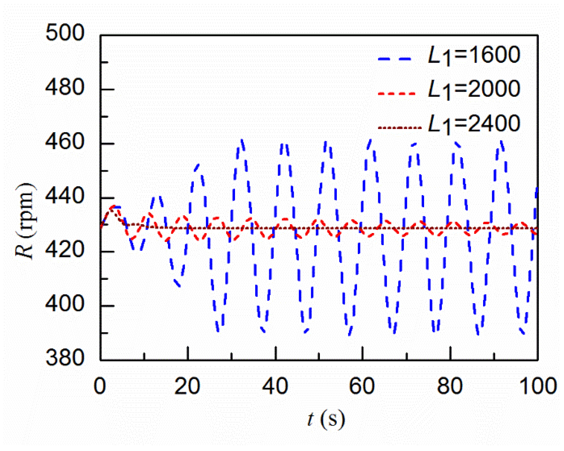
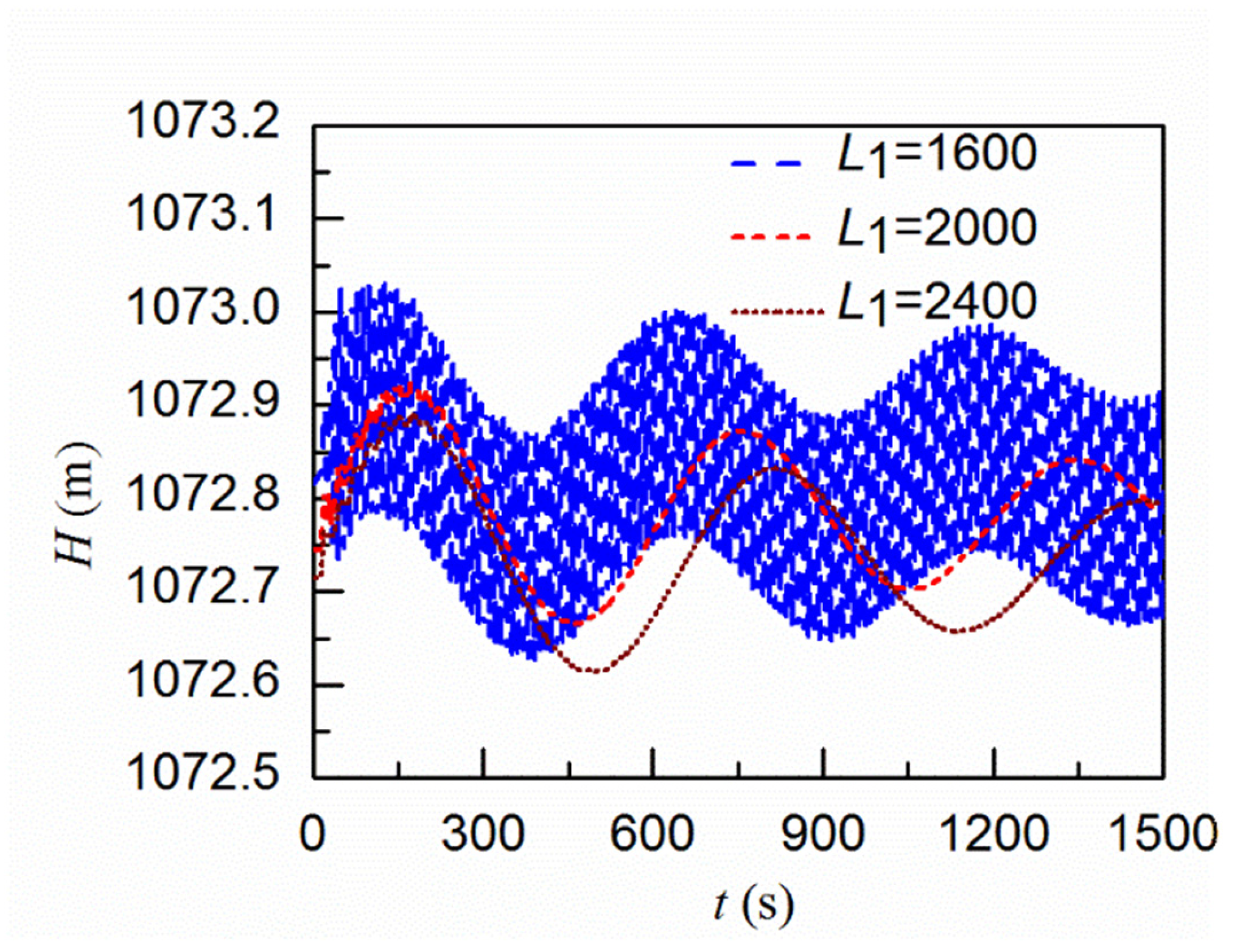
In this case, the loads of all the turbines are reduced by 5% simultaneously. The guide vanes of the turbines are controlled by the servomotor with a frequency regulation process. The parameters of the controller are shown in Table 2 with the assumed zero load self-regulation coefficient of the power grid. The details of the controller can be found in [3]. Three scenarios with L1 = 1600 m, 2000 m and 2400 m, respectively, were simulated to illustrate the effects of the position of the sand basin on the transient process. The rotational speed of the turbine and the water level in the sand basin for these three scenarios are compared in Figure 14 and Figure 15, respectively. Similar to having a surge tank in the system, the comparisons show that a shorter distance between the sand basin and the turbines can facilitate the stability of the transient process.
4.3.2. Comparison with the Results by Modelling the Basin Tank as a Surge Tank
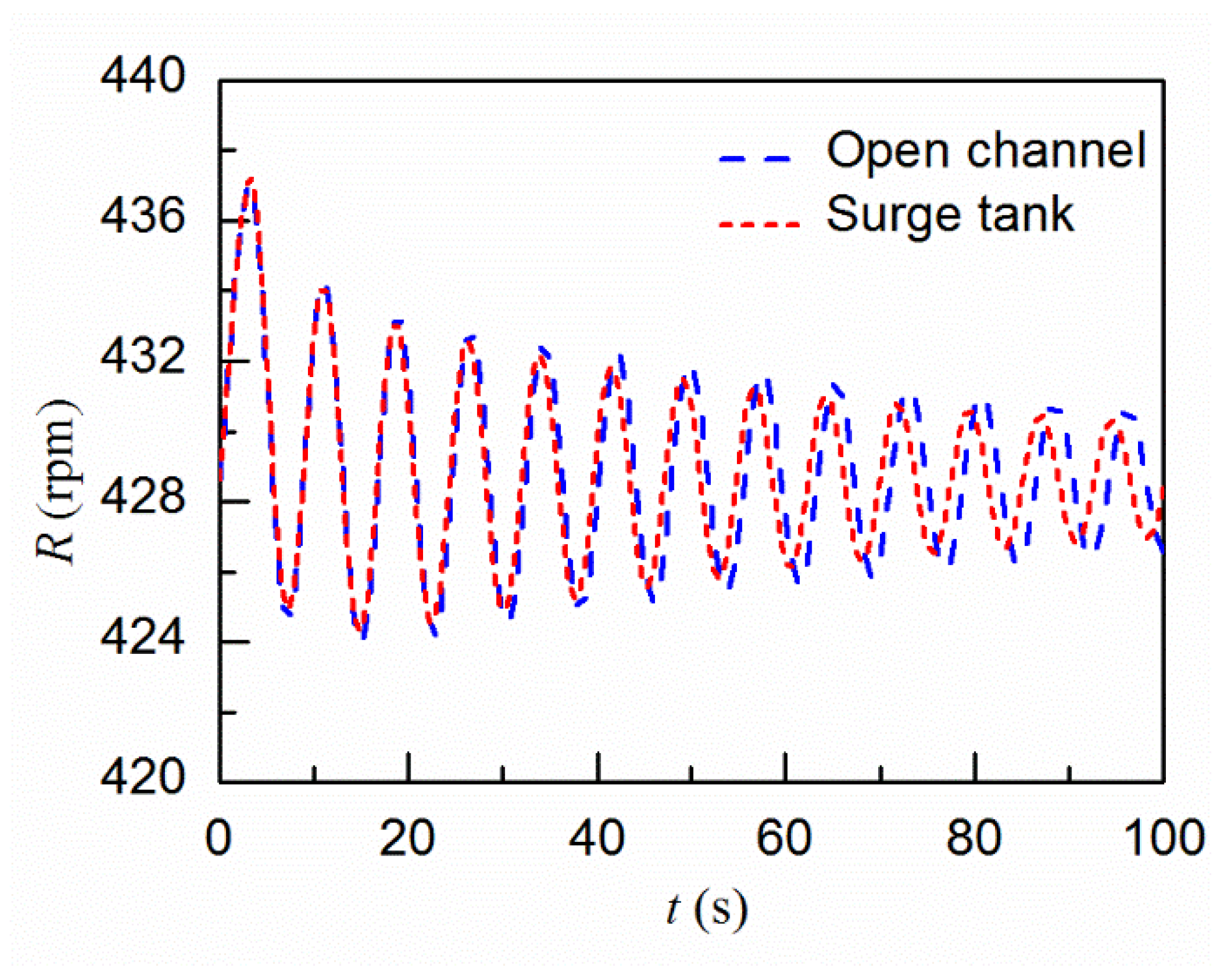
With L1 = 2000 m, the simulated rotational speed of the turbine and the water level fluctuations in the sand basin are shown in Figure 16 and Figure 17, respectively. They are also compared with the results by modelling the sand basin as an open channel. Similar to the full load rejection simulation, the differences observed in the comparison can be ascribed to the neglected flow velocity and friction in the sand basin along the horizontal direction in the surge tank modelling. It can be concluded that treating the sand basin as a surge tank in the modelling may overestimate the operation stability of the system.
5. Conclusions
A MOC-FVM coupling method is developed in this paper to simulate pipeline-open channel coupling transient flow in hydraulic systems including hydropower systems. Pipelines in the systems are modelled using the MOC and the open channel is modelled using the 1D FVM. The coupling boundaries between the MOC simulation region and the FVM simulation region are developed based on Riemann invariants. 3D CFD simulation on a tank-pipe system has been conducted with the result almost identical to that simulated by the proposed coupling method. The proposed method is then applied to a prototype hydropower station with a constructed sand basin. The main conclusions include:
- The MOC-FVM coupling method can accurately simulate the pipeline-open channel coupling transient flow with the simulated parameters transmitted successfully at the coupling boundaries.
- The coupling method has been successfully applied to a hydropower station with a sand basin constructed between the upstream reservoir and turbines. The sand basin can be modelled as an open channel.
- The effects of the sand basin on the transient process are similar to a surge tank which can relieve water hammer pressures during load rejection scenarios and can benefit the frequency regulation process. By modelling the sand basin as an open channel, the flow velocity and the friction in the horizontal direction, which are neglected when modelling the sand basin as a surge tank, can be considered, and thus more reliable and accurate results can be obtained.
Author Contributions
Conceptualization, C.W., W.Z. and J.Y.; methodology, C.W. and W.Z.; software, C.W.; validation, C.W. and J.Y.; investigation, C.W. and W.Z.; writing—original draft preparation, W.Z.; writing—review and editing, C.W. and J.Y.; supervision, J.Y. All authors have read and agreed to the published version of the manuscript.
Funding
The research presented in this study was funded by the Open Research Fund Program of the State Key Laboratory of Water Resources and Hydropower Engineering Science (Grant 2017SDG01), China.
Institutional Review Board Statement
Not applicable.
Informed Consent Statement
Not applicable.
Data Availability Statement
Not applicable.
Acknowledgments
Not applicable.
Conflicts of Interest
The authors declare no conflict of interest.
References
- Kim, S.-G.; Lee, K.-B.; Kim, K.-Y. Water hammer in the pump-rising pipeline system with an air chamber. J. Hydrodyn. 2014, 26, 960–964. [Google Scholar] [CrossRef]
- Zhang, K.; Zeng, W.; Simpson, A.R.; Zhang, S.; Wang, C. Water Hammer Simulation Method in Pressurized Pipeline with a Moving Isolation Device. Water 2021, 13, 1794. [Google Scholar] [CrossRef]
- Yang, W.; Yang, J.; Guo, W.; Zeng, W.; Wang, C.; Saarinen, L.; Norrlund, P. A Mathematical Model and Its Application for Hydro Power Units under Different Operating Conditions. Energies 2015, 8, 10260–10275. [Google Scholar] [CrossRef]
- Karpenko, M.; Bogdevicius, M. Investigation into the hydrodynamic processes of fitting connections for determining pressure losses of transport hydraulic drive. Transport 2020, 35, 108–120. [Google Scholar] [CrossRef]
- Wylie, E.B.; Streeter, V.L. Fluid Transients in Systems; Prentice Hall Inc.: Englewood Cliffs, NJ, USA, 1993. [Google Scholar]
- Urbanowicz, K. Modern Modeling of Water Hammer. Pol. Marit. Res. 2017, 24, 68–77. [Google Scholar] [CrossRef]
- Chaudhry, M.H. Applied Hydraulic Transients, 3rd ed.; Springer: New York, NY, USA, 2014. [Google Scholar]
- Nicolet, C. Hydroacoustic Modelling and Numerical Simulation of Unsteady Operation of Hydroelectric Systems. Ph.D. Thesis, École Polytechnique Fédérale de Lausanne, Lausanne, Switzerland, 2007. [Google Scholar]
- Tijsseling, A.S. Fluid-structure interaction in liquid-filled pipe systems: A review. J. Fluids Struct. 1996, 10, 109–146. [Google Scholar] [CrossRef]
- Covas, D.; Stoianov, I.; Mano, J.F.; Ramos, H.; Graham, N.; Maksimovic, C. The dynamic effect of pipe-wall viscoelasticity in hydraulic transients. Part I—Experimental analysis and creep characterization. J. Hydraul. Res. 2004, 42, 516–530. [Google Scholar] [CrossRef]
- Vardy, A.E.; Brown, J.M.B. Transient, turbulent, smooth pipe friction. J. Hydraul. Res. 1995, 33, 435–456. [Google Scholar] [CrossRef]
- Lai, W.; Khan, A.A. Numerical solution of the Saint-Venant equations by an efficient hybrid finite-volume/finite-difference method. J. Hydrodyn. 2018, 30, 189–202. [Google Scholar] [CrossRef]
- Guo, Y.; Liu, R.-X.; Duan, Y.-L.; Li, Y. A Characteristic-Based Finite Volume Scheme for Shallow Water Equations. J. Hydrodyn. 2009, 21, 531–540. [Google Scholar] [CrossRef]
- Yin, C.-C.; Zeng, W.; Yang, J.-D. Transient simulation and analysis of the simultaneous load rejection process in pumped storage power stations using a 1-D-3-D coupling method. J. Hydrodyn. 2021, 33, 979–991. [Google Scholar] [CrossRef]
- Wang, C.; Nilsson, H.; Yang, J.; Petit, O. 1D–3D coupling for hydraulic system transient simulations. Comput. Phys. Commun. 2017, 210, 1–9. [Google Scholar] [CrossRef]
- Zhang, X.-X.; Cheng, Y.-G.; Yang, J.-D.; Xia, L.-S.; Lai, X. Simulation of the load rejection transient process of a francis turbine by using a 1-D-3-D coupling approach. J. Hydrodyn. 2014, 26, 715–724. [Google Scholar] [CrossRef]
- Zhang, X.-X.; Cheng, Y.-G. Simulation of Hydraulic Transients in Hydropower Systems Using the 1-D-3-D Coupling Approach. J. Hydrodyn. 2012, 24, 595–604. [Google Scholar] [CrossRef]
- Yang, J.; Yang, J. 1-D MOC simulation software for hydraulic transients: TOPsys. Proc. IOP Conf. Ser. Earth Environ. Sci. 2018, 163, 12081. [Google Scholar] [CrossRef]
- Zeng, W.; Yang, J.; Hu, J. Pumped storage system model and experimental investigations on S-induced issues during transients. Mech. Syst. Signal Pract. 2017, 90, 350–364. [Google Scholar] [CrossRef]
- Hu, J.; Yang, J.; Zeng, W.; Yang, J. Transient Pressure Analysis of a Prototype Pump Turbine: Field Tests and Simulation. J. Fluids Eng. 2018, 140, 71102. [Google Scholar] [CrossRef]
- Wang, C.; Yang, J.-D. Water Hammer Simulation Using Explicit-Implicit Coupling Methods. J. Hydraul. Eng. 2015, 141, 4014086. [Google Scholar] [CrossRef]
- Toro, E.F. Shock-Capturing Methods for Free-Surface Shallow Flows; Wiley: Hoboken, NJ, USA, 2001. [Google Scholar]
- Toro, E.F. Riemann Solvers and Numerical Methods for Fluid Dynamics: A Practical Introduction; Springer Science & Business Media: Berlin/Heidelberg, Germany, 2013. [Google Scholar]
Figure 1.
Characteristics lines in the x-t plane.

Figure 2.
The schematic of the FVM grids.

Figure 3.
The calculation process of the coupling method represented by grids.

Figure 4.
Schematic of the tank-pipe system.

Figure 5.
Comparison of the simulated results by the MOC-FVM coupling method and the 3D FVM.

Figure 6.
Schematic of the hydropower station with a sand basin.

Figure 7.
Modelling of the hydropower system in TOPSYS.

Figure 8.
Comparison of the pressure heads at the inlet of the spiral case with different positions of the sand basin.
Figure 8.
Comparison of the pressure heads at the inlet of the spiral case with different positions of the sand basin.

Figure 9.
Comparison of the pressure heads at the inlet of the spiral case with different sizes of the sand basin.
Figure 9.
Comparison of the pressure heads at the inlet of the spiral case with different sizes of the sand basin.

Figure 10.
Comparison of the water levels in the sand basin with different sizes of the sand basin (L1 = 2400 m).
Figure 10.
Comparison of the water levels in the sand basin with different sizes of the sand basin (L1 = 2400 m).

Figure 11.
Comparison of the water levels in the sand basin at different positions (L1 = 2400 m, h = 10 m, w = 10 m).
Figure 11.
Comparison of the water levels in the sand basin at different positions (L1 = 2400 m, h = 10 m, w = 10 m).

Figure 12.
Comparison of the water levels in the sand basin with different modelling methods (L1 = 2400 m, h = 10 m, w = 10 m).
Figure 12.
Comparison of the water levels in the sand basin with different modelling methods (L1 = 2400 m, h = 10 m, w = 10 m).

Figure 13.
Comparison of the water levels in the sand basin with different modelling methods (L1 = 400 m, h = 10 m, w = 10 m).
Figure 13.
Comparison of the water levels in the sand basin with different modelling methods (L1 = 400 m, h = 10 m, w = 10 m).

Figure 14.
Comparison of the turbine rotational speed with different locations of the sand basin (h = 10 m, w = 10 m).
Figure 14.
Comparison of the turbine rotational speed with different locations of the sand basin (h = 10 m, w = 10 m).

Figure 15.
Comparison of the water level fluctuations in the sand basin with different locations of the sand basin (h = 10 m, w = 10 m).
Figure 15.
Comparison of the water level fluctuations in the sand basin with different locations of the sand basin (h = 10 m, w = 10 m).

Figure 16.
Comparison of the turbine rotational speed with different modelling methods (L1 = 2000 m, h = 10 m, w = 10 m).
Figure 16.
Comparison of the turbine rotational speed with different modelling methods (L1 = 2000 m, h = 10 m, w = 10 m).

Figure 17.
Comparison of the water level fluctuations in the sand basin with different modelling methods (L1 = 2000 m, h = 10 m, w = 10 m).
Figure 17.
Comparison of the water level fluctuations in the sand basin with different modelling methods (L1 = 2000 m, h = 10 m, w = 10 m).


Table 1.
Basic information about the hydropower station.
| Runner Inlet Diameter (m) | Guide Vane Height (m) | Upstream Water Level (m) | Downstream Water Level (m) | Rated Rotational Speed (rpm) | Rated Output (Mw) | Rated Flow Rate (m3/s) | Rotational Inertia (t.m2) |
|---|---|---|---|---|---|---|---|
| 2.3 | 0.7 | 1073 | 829 | 429.6 | 10.54 | 29 | 726 |
Table 2.
Parameter setting for the PID controller.
| Temporary Droop | Differential Time Constant | Time Lag in Servomotor | Dashpot Time Constant |
|---|---|---|---|
| 0.3 | 0.3 s | 0.05 s | 5.0 s |
Publisher’s Note: MDPI stays neutral with regard to jurisdictional claims in published maps and institutional affiliations. |
© 2022 by the authors. Licensee MDPI, Basel, Switzerland. This article is an open access article distributed under the terms and conditions of the Creative Commons Attribution (CC BY) license (https://creativecommons.org/licenses/by/4.0/).
Share and Cite
MDPI and ACS Style
Zeng, W.; Wang, C.; Yang, J. Hydraulic Transient Simulation of Pipeline-Open Channel Coupling Systems and Its Applications in Hydropower Stations. Water 2022, 14, 2897. https://doi.org/10.3390/w14182897
AMA Style
Zeng W, Wang C, Yang J. Hydraulic Transient Simulation of Pipeline-Open Channel Coupling Systems and Its Applications in Hydropower Stations. Water. 2022; 14(18):2897. https://doi.org/10.3390/w14182897
Chicago/Turabian StyleZeng, Wei, Chao Wang, and Jiandong Yang. 2022. "Hydraulic Transient Simulation of Pipeline-Open Channel Coupling Systems and Its Applications in Hydropower Stations" Water 14, no. 18: 2897. https://doi.org/10.3390/w14182897
Note that from the first issue of 2016, this journal uses article numbers instead of page numbers. See further details here.