Article

Evaluation of Machine Learning Models for Daily Reference Evapotranspiration Modeling Using Limited Meteorological Data in Eastern Inner Mongolia, North China

1
College of Agriculture, Shenyang Agricultural University, Shenyang 110866, China
2
Chifeng Institute of Agricultural and Animal Husbandry Science, Chifeng 024031, China
3
Farmland Irrigation Research Institute, Chinese Academy of Agriculture Sciences, Xinxiang 453003, China
*
Authors to whom correspondence should be addressed.
Water 2022, 14(18), 2890; https://doi.org/10.3390/w14182890
Submission received: 9 August 2022 / Revised: 12 September 2022 / Accepted: 13 September 2022 / Published: 16 September 2022

Abstract

:
Background: Water shortages limit agricultural production in arid and semiarid regions around the world. The accurate estimation of reference evapotranspiration (ET0) is of the utmost importance for computing crop water requirements, agricultural water management, and irrigation scheduling design. However, due to the combination of insufficient meteorological data and uncertain inputs, the accuracy and stability of the ET0 prediction model were different to varying degrees. Methods: Six machine learning models were proposed in the current study for daily ET0 estimation. Information on the weather, such as the maximum and minimum air temperatures, solar radiation, relative humidity, and wind speed, during the period 1960~2019 was obtained from eighteen stations in the northeast of Inner Mongolia, China. Three input combinations were utilized to train and test the proposed models and compared with the corresponding empirical equations, including two temperature-based, three radiation-based, and two humidity-based empirical equations. To evaluate the ET0 estimation models, two strategies were used: (1) in each weather station, we trained and tested the proposed machine learning model, and then compared it with the empirical equations, and (2) using the K-means algorithm, all weather stations were sorted into three groups based on their average climatic features. Then, each station tested the machine learning model trained using the other stations within the group. Three statistical indicators, namely, determination coefficient (R2), root mean square error (RMSE), and mean absolute error (MAE), were used to evaluate the performance of the models. Results: The results showed the following: (1) The temperature-based temporal convolutional neural network (TCN) model outperformed the empirical equations in the first strategy, as shown by the TCN’s R2 values being 0.091, 0.050, and 0.061 higher than those of empirical equations; the RMSE of the TCN being significantly lower than that of empirical equations by 0.224, 0.135, and 0.159 mm/d; and the MAE of the TCN being significantly lower than that of empirical equations by 0.208, 0.151, and 0.097 mm/d, and compared with the temperature-based empirical equations, the TCN model markedly reduced RMSE and MAE while increasing R2 in the second strategy. (2) In comparison to the radiation-based empirical equations, all machine learning models reduced RMSE and MAE, while significantly increasing R2 in both strategies, particularly the TCN model. (3) In addition, in both strategies, all machine learning models, particularly the TCN model, enhanced R2 and reduced RMSE and MAE significantly when compared to humidity-based empirical equations. Conclusions: When the radiation or humidity characteristics were added to the given temperature characteristics, all the proposed machine learning models could estimate ET0, and its accuracy was higher than the calibrated empirical equations external to the training study area, which makes it possible to develop an ET0 estimation model for cross-station data with similar meteorological characteristics to obtain a satisfactory ET0 estimation for the target station.

1. Introduction

Optimizing the use of the limited available water, especially in agricultural production systems, is becoming increasingly crucial in recent years due to the rising demand for water resources as a consequence of uneven water distribution, resource abuse, and inefficient irrigation practices. Therefore, in order to manage the increasingly precious water resources, it is vital to study various techniques to enhance water efficiency and prevent excessive water consumption. Crop evapotranspiration (ET), which is crucial in tasks such as irrigation scheduling and forecasting, water resource management, agricultural water resource development, and hydrological studies, is based on the accurate estimation of reference evapotranspiration (ET0) [1,2,3]. As a result of the high accuracy across a range of climatic circumstances, the United Nations Food and Agriculture Organization (FAO) has recommended the Penman–Monteith equation (FAO56-PM) as a standard approach for predicting ET0 and calibrating other empirical and semiempirical models [4,5,6]. The FAO56-PM equation data requirements, however, are high, since the model requires solar radiation, the maximum and minimum air temperature, relative humidity, and wind speed. The meteorological stations measuring these features, worldwide, are scarce, and the wide application of the Penman–Monteith method has thus been severely constrained, especially in developing countries such as China [7]. Therefore, in order to estimate ET0 accurately, a simpler model using fewer weather feature inputs needs to be explored.
Numerous methods depending upon incomplete weather characteristics have been developed to estimate ET0, such as temperature-based models [8,9], radiation-based models [10,11,12], humidity-based models [13,14], mass transfer-based models [15], and pan-based methods [16]. Among these models, when all meteorological features are unavailable, the first three models are frequently used to replace the FAO56-PM equation to calculate ET0 [10]. Nevertheless, these empirical models also have some defects, such as either overestimating or underestimating the ET0 [14], and are suitable to estimate weekly or monthly scales but not effective for daily ET0 estimation [17]. Thus, it is necessary to investigate and develop better models for forecasting ET0 with a high level of precision using fewer weather features.
In recent decades, with advancements in artificial intelligence and data mining technology, some scholars have begun to apply machine learning models and deep learning models to estimate ET0 in order to overcome the dependency on meteorological data due to their outstanding capacity to handle nonlinear interactions between the dependent and independent variables. To forecast ET0, many machine learning and deep learning models have been proposed, including support vector machines (SVMs) [18,19,20], random forests (RFs) [5,21], the M5 model tree (M5Tree) [22,23], extreme gradient boosting (XGBoost) [24], artificial neural networks (ANNs) [4,25], extreme learning machines (ELMs) [7,26], the long short-term memory neural network (LSTM) [16,27], bidirectional LSTM (Bi-LSTM) [28], the adaptive neuro fuzzy inference system (ANFIS) [29], and multivariate adaptive regression spline (MARS) [30,31].
The linked study makes clear that the ANN, SVM, and RF models have been employed extensively for ET0 prediction, but the employment of deep machine learning methods, particularly the TCN and LSTM models, have been quite sparse. In addition, there has not been a thorough comparison of these deep learning models with the widely used ANN, SVM, and RF models, particularly in terms of their performance in predicting ET0 with limited meteorological inputs under different climatic conditions. Additionally, almost all studies that have adopted classical machine learning models (e.g., ANN, SVM and RF) to estimate ET0 have tested the accuracy and stability of these models for forecasting ET0 in a single station alone, which fails to make a comparison with machine learning models. In this case, the specific objectives of this study were to (1) develop six machine learning models, namely, TCN, ANN, LSTM, K-nearest neighbors (KNN), RF, and Light Gradient-Boosting Machine (LGB), to predict ET0 in North China’s Inner Mongolia Autonomous Region; (2) determine the effects of limited meteorological inputs on the accuracy of daily ET0 prediction; and (3) investigate the performance of these machine learning models and empirical equations within and outside of the study area.

2. Materials and Methods

As shown in Figure 1, the study region is located in the northeast of the Inner Mongolia Autonomous Region (41°17′ N~53°20′ N; 115°31′ E~126°4′ E), China. Three-quarters of the grain produced in the Inner Mongolia Autonomous Region was produced in this region, which has an area of approximately = 0.462 million km2. With features of both a continental and monsoon climate, the northeast of the Inner Mongolia Autonomous Region is in the mild temperate zone. The average daily weather variables for the 18 stations located in the northeast of China’s Inner Mongolia Autonomous Region are summarized in Table 1. Continuous daily meteorological data during the period 1960–2019 were collected from the China Meteorological Administration in this study, including maximum temperature (Tmax), minimum temperature (Tmin), sunshine duration (SH), relative humidity (RH), wind speed at 2 m height (U2), and precipitation (P).

2.1. Models for Modeling Reference Evapotranspiration

2.1.1. FAO-56 Penman–Monteith Equation

The FAO-recommended Penman–Monteith equation (FAO 56-PM) was used to estimate ET0 data, which were chosen as the calibration and assessment goals for the proposed models. This process is reasonable and has been applied in many earlier investigations [4,32,33,34]. The following shows how the Penman–Monteith model is expressed:
ET 0 = 0.408 ( R n G ) + γ 900 T + 273 u 2 ( e s e a ) + γ ( 1 + 0.34 u 2 )
where ET 0 is the reference evapotranspiration (mm d−1); R n is the net radiation (MJm−2d−1); G is the soil heat flux density (MJm−2d−1); T is the mean daily air temperature (°C); u2 is the wind speed at a height of 2 m (ms−1); es and ea are the saturation vapor pressure (kPa) and actual vapor pressure (kPa), respectively; is the slope vapor pressure curve (kPa °C−1); and γ is the psychrometric constant (kPa °C−1).

2.1.2. Empirical Models for Predicting Daily ET0

Temperature-based empirical models. When statistics on solar radiation, relative humidity, and wind speed are lacking, the Hargreaves model and modified Hargreaves model predict daily ET0 using just the maximum and minimum air temperature. Equations (2)–(4) represent the Hargreaves and modified Hargreaves models, respectively [8,35,36].
ET 0 = 0.000939 ( T avg + 17.8 ) ( T max T min ) 0.5 R a
ET 0 = 0.000939 ( T avg + 37.5 ) ( T max T min ) 0.424 R a
ET 0 = 0.000816 ( T avg + 33.9 ) ( T max T min ) 0.296 R a
where T max is the maximum air temperature (°C); T min is the minimum air temperature (°C); T avg is calculated as the average of T max and T min (°C); and R a is the extraterrestrial radiation for daily periods (MJm−2d−1), which is calculated using the following equation:
R a = 24 × 60 π G SC d r [ ( ω s sin ( φ ) sin ( δ ) + cos ( φ ) cos ( δ ) sin ( ω s ) ]
where G SC denotes a solar constant that is equal to 0.0820 MJm−2min−1; d r is the inverse relative distance between the Earth and the sun; δ is the solar declination (rad); φ is the latitude (rad); ω s is the sunset hour angle (rad).
Radiation-based models. The Ritchie (Equation (6)), Priestley–Taylor (Equation (7)), and Makkink (Equation (8)) models—three widely used and highly accurate radiation-based models that call for information on air temperature and solar radiation—were employed to calculate ET0 [10,11,37].
ET 0 = a 1 × [ 0.00387 R s ( 0.6 T max + 0.4 T min + 29 ) ]
When
5   <   T max   >   35   ° C   a 1 = 1.1 ; T max   >   35   ° C   a 1 = 1.1 + 0.05 ( T max 35 ) ; T max   <   5   ° C   a 1 = 0.01 exp ( T max + 20 ) .
ET 0 = 1.26 + γ ( R n G )
ET 0 = 0.61 + γ R s 0.12
where R s is the solar radiation, and R s in MJm−2d−1 is given by
R s = a s + b s n N R a
where n is the actual duration of sunshine (hour); N is the maximum possible duration of sunshine or daylight hours (hour); a s and b s are the regression constants; and the values a s = 0.25 and b s = 0.5.
Humidity-based models. Two empirical equations based on relative humidity and temperature data, Romanenko (R) and Schendel (S) equations, were applied in this work [13,14]. These equations have often been applied in the literature by many researchers. Equations (10) and (11) represent the R and S equations, respectively.
ET 0 = 0.00006 ( 25 + T avg ) 2 ( 100 RH )
ET 0 = 16 T avg RH  
where T avg is the mean air temperature, °C, and RH is the mean air relative humidity.
In accordance with the advice of Allen et al. and the investigations of various authors [5,38,39], the empirical methods were calibrated using statistics from all weather stations under study based on a simple linear model. Calibrated ET0 was derived using the following formula:
ET 0 , cal = aET 0 + b
where ET 0 , cal is the reference evapotranspiration calculated using the calibrated equation, and a and b are the calibration parameters.

2.1.3. Machine Learning Models for Predicting Daily ET0

Random forest (RF). An ensemble of numerous classification or regression trees known as a “random forest” (RF) model aims to create precise predictions that do not overfit the data. It is a combination of tree predictors that depend on the values of random vectors sampled independently and with the same distribution for all trees in the forest [40]. Great prediction accuracy and high tolerance for outliers and “noise” have both been demonstrated in the RF model. The RF model produces n data sets from the original data set’s duplicate samples. It creates an unpruned classification or regression tree for each dataset. All trees vote to determine the final categorization outcome for the classification issue. However, the average of all the tree outcomes is the ultimate solution for the regression problem.
K-nearest neighbors (KNN). The K-nearest neighbors (KNN) is a nonparametric regression method which is different from the traditional regression method [41]. The KNN regression does not have a fixed function form and predicts the values for test data/new data points by looking for similar testing state samples among historical data. The similarity of the new point to the training data samples determines its value. There are two methods for KNN regression. The average of the target of the K-nearest neighbors is first calculated. The second calculation is the inverse distance weighted average of the K-nearest neighbors [42]. KNN regression uses the same distance functions as KNN classification—Euclidean, Manhattan, and Minkowski. Due to its simplicity and intuitiveness, KNN is widely adopted for classification and regression [43,44].
Light Gradient-Boosting Machine (LGB). LGB is a novel GBDT (gradient-boosting decision tree) algorithm, proposed by Microsoft, which has been used in many different kinds of data mining tasks, such as classification and regression [45]. The LGB algorithm contains two novel techniques, which are gradient-based one-side sampling and exclusive feature bundling, respectively. Gradient-based one-side sampling (GOSS) can eliminate a large amount of data with a small gradient, and only uses the remaining data to estimate the information gain, so as to avoid the influence of the long tail of the low gradient. Exclusive feature bundling (EFB) implements the binding of mutually exclusive features to reduce the number of features. Additionally, the histogram-based algorithms can help speed up training and reduce memory usage. More importantly, compared with traditional parallel methods, LGB also has feature parallel and data parallel advantages. LGB’s remarkable prediction accuracy has led to its widespread use in a variety of sectors, preventing the model from overfitting during training; greatly speeding up the forecasting speed; and reducing its memory utilization [46,47,48].
Artificial neural networks (ANNs). An artificial neural network (ANN) is a type of information processing system that mimics the capacity of the human brain to recognize patterns and learn from mistakes. ANNs generally have a number of processing components called neurons that are connected by synaptic weights [26]. Typically, an ANN’s design consists of an input layer, some hidden layers, and an output layer. The input layer and output layer denote the inputs and output, respectively. The function of hidden layers is to complicate the ANN, which is necessary for solving nonlinear fitting problems.
In the ANN model, every neuron receives weighted inputs, which might be input variables or the outputs of the neuron in the preceding layer. The inputs are then summed, a bias term is added, and the outcome is sent through an activation function to produce the output (activation value). The required output can be generated by modifying the weights of an artificial neuron. The operation of adjusting the weights of the ANN is called learning or training. Additionally, a number of learning algorithms, such as the backpropagation algorithm, radial basis function, generalized regression, conjugate gradient descent, and quick propagation, try to minimize the error function of the ANN model. The backpropagation algorithm is the most frequently used among them. This algorithm is trained using sets of examples that contain input arrays and the desired output arrays. The input is introduced to the network, and the error between the actual and desired output is then propagated backward in the network to readjust the weights in order to reduce the error. In this study, we adopted a backpropagation algorithm to train an ANN model, and then used it for estimating ET0.
Long short-term memory (LSTM). LSTM is an excellent variant of the recurrent neural network (RNN), which solves the problem of gradient disappearance and difficult training of RNN [49]. The LSTM is a nonlinear time series model that can learn the order dependency between observations in a sequence and allows information to persist using a memory state. The core idea of LSTM is the state of the cell, which introduces a hidden layer unit known as a memory cell compared to the traditional RNN. Three gates—the input gate, output gate, and forget gate—are used by memory cells to govern their self-connections, which store the network’s temporal state for later use. The memory cell has the ability to store historical information and recall it at any time. The cell allows the network to only remember, store, and transfer information that is directly connected to the current value and to forget other information that is not relevant. As a result, LSTMs do not struggle to learn new information; rather, long-term memory is basically their default habit.
Temporal convolutional neural network (TCN). The temporal convolutional neural network (TCN) approach was initially developed to examine long-range patterns using a hierarchy of temporal convolutional filters [50]. The TCN is founded on two guiding principles: first, that knowledge about the future cannot be revealed in the past and, second, that a neural network will always create an output that is as long as its input. Causal convolution is introduced to meet these two criteria. In causal convolution, only the neural nodes that are active at time step t and those that were active previously in the prior layer are convolved. The lengthy sequence, however, complicates the simple causal convolution. To look back in time for very long time sequences, we need to stack causal convolution for several layers. However, this procedure will result in overfitting and a significant rise in parameters. Dilated convolution is offered as a solution to this issue. Another crucial component of TCN is residual connection. According to residual connection, the input of the block is increased by the output of a branch that includes a number of transformations. The TCN is defined as 1D causal CNN + 1D dilation CNN + residual connection, in brief. These techniques allow TCN to extract data from multivariate time sequences with a minimal number of layers while maintaining the temporal characteristic.

2.2. Data Management and the Development of Machine Learning Models

This study investigated the performance of the suggested empirical and machine learning models for calculating ET0 with incomplete meteorological data under three data availability situations: temperature-based models, which used only measured data on maximum and minimum air temperature; humidity-based models, which used measured data on maximum and minimum air temperature, average temperature, and relative humidity; and radiation-based models, which used measured data on maximum and minimum air temperature, average temperature, and solar radiation. In these instances, extraterrestrial radiation, which was estimated using latitude and the day of the year, was applied to supplement the observed data [39]. Furthermore, the differences in performance between the proposed machine learning models and the relevant empirical equations were tested individually for significance.
In order to obtain models with higher performances, we used the K-means method to group weather stations according to their average climatic characteristics: Group I had 8 weather stations, Group II had 6 weather station, and Group III included 4 weather stations, as presented in Table 1, and then two methodologies were also used. The first strategy involved training and testing all machine models in every single weather station in each group. The second strategy was for each station in each group to take turns serving as a validation station, testing the models trained by the other stations within the group. Meteorological data from all of the weather stations in each group were used to build the models. In the first strategy, taking into account that the performance of the model in a single weather station could not be used to determine whether the model was superior, these data were randomized and split into training (75%) and validation (25%) sets. The t-test was used in both strategies to evaluate whether there were any significant variations in how well the proposed models performed.
For each weather station, the daily average values of Tmax, Tmin, RH, Ra, Rs, and ET0 from 1960 to 2019 were available for this study. All weather stations were grouped using these features via the K-means algorithm, a well-known clustering technique that has the advantages of being quick and simple. K-means is one of the most commonly used data clustering algorithms, and its wide application is well-known. Given K initial centroids, the K-means algorithm aims to assign algorithms of the data points into K clusters by minimizing the distance from each vector to the centroid of its cluster. Therefore, it produced various clustering outcomes with various cluster numbers and initial centroid values. Since choosing the K value is not an easy task, the best choice of K value was determined using the silhouette coefficient. The value of the silhouette coefficient is between −1 and 1: the closer to 1, the better the cohesion and separation. Figure 2 demonstrates that the study’s best option was the use of three clusters, with a silhouette coefficient of 0.57. Table 1 displays the K-means algorithm’s output, which shows that Eergunaqi, Tulihe, Xiaoergou, and Aershan belonged to Group III; Manzhouli, Hailaer, Xinbaerhuyouqi, Xinbaerhuzuoqi, Zhalantun, and Suolun belonged to Group II; and the others belonged to Group I.
Before the training of the machine learning models, original meteorological data were normalized as input variables ranging from 0 to 1 according to Equation (13) to avoid convergence problems.
x n = x i x min x max x min
where xn and xi represent the moralized and raw training and testing data, respectively, and xmax and xmin are the minimum and maximum of the training and testing data, respectively.

2.3. Model Performance and Assessment

Three commonly used statistical indicators—the determination coefficient (R2), root mean square error (RMSE), and mean absolute error (MAE)—were used to assess and compare the performance of the trained models for estimating ET0. The formulae are as follows:
R 2 = [ i = 1 N ( O i O ¯ ) ( P i P ¯ ) i = 1 N ( O i O ¯ ) 2 i = 1 N ( P i P ¯ ) 2 ] 2
RMSE = 1 N i = 1 N ( P i O i ) 2
MAE = 1 N i = 1 N | O i P i |  
where Oi is the ith observation (mm/d), Pi is the predicted value of the ith model (mm/d), O ¯ is the average of the observed values Oi (mm/d), P ¯ is the average of the model-predicted values Pi (mm/d), and N is the number of samples.

3. Results

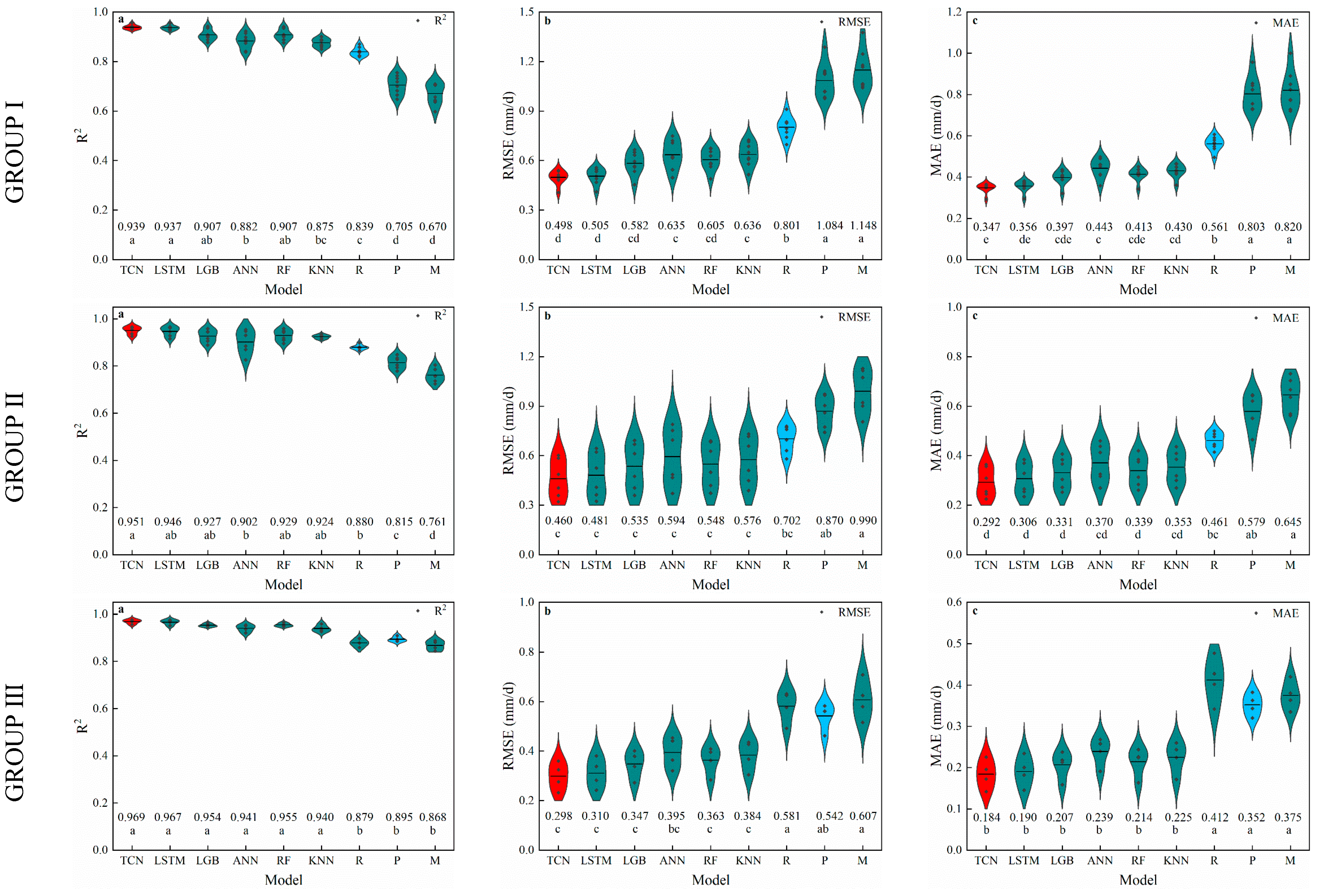
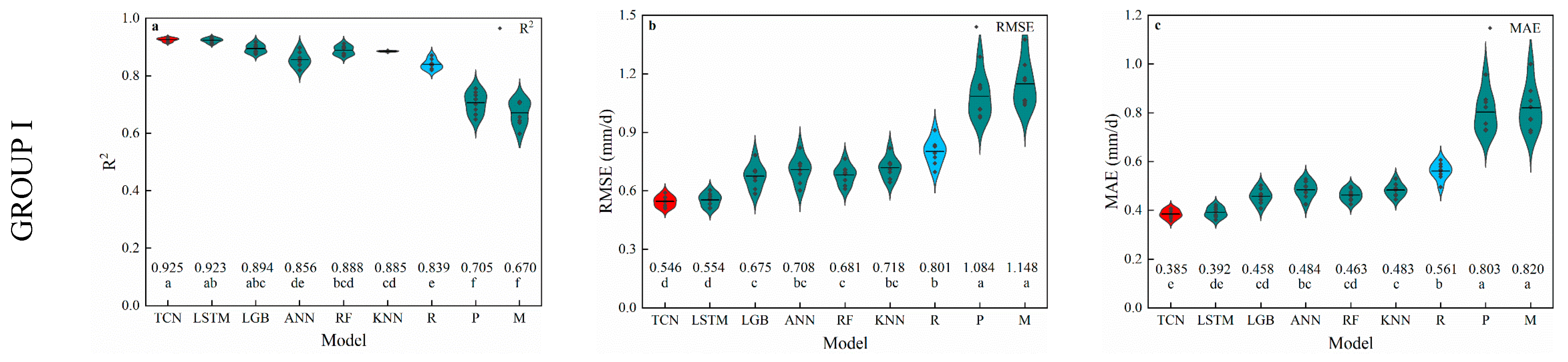
3.1. Temperature-Based Models

The statistical results of the six machine learning models for estimating ET0 in the first strategy are provided in Figure 3. According to Figure 3, the mean R2 of the H model was higher than that of MH1 and MH2, and the RMSE and MAE were lower than those of MH1 and MH2 in the first and second groups. However, for the third group, the mean R2 of MH2 was higher, and the RMSE and MAE were lower. Thus, the prediction accuracy of TCN, LSTM, LGB, ANN, RF, and KNN, based on air temperature data, was compared with H in the first and second groups, and with MH2 in the third group.
Compared with the H model, the R2 of ANN and KNN was not significantly different, but both the RMSE and MAE were lower than those of the H model in the first group. Figure 3 also illustrates that the TCN, LSTN, LGB, and RF all performed similarly better than the H model, with a significant increase in the mean R2 values ranging from 0.054 to 0.091, and a significant reduction in RMSE, 0.115–0.224 mm/d, and MAE, 0.39–0.208 mm/d, respectively. In the second group, the ANN and KNN models performed as well as the H model, while the LSTM, LGB, and RF models performed better than the H model, with a decrease in MAE of 0.131, 0.126, and 0.106 mm/d, respectively. The mean R2 value of the TCN was 0.920, which was 0.05 higher than that of H, and the MAE of the TCN was 0.379 mm/d, which was 0.151 mm/d lower than that of H. For the third group, from the general trend of R2, RMSE, and MAE, only the TCN model had a better performance among all machine learning models, with an R2 of 0.935, RMSE of 0.433 mm/d, and MAE of 0.277 mm/d. These results indicated that, in the three groups, the temperature-based TCN model outperformed the empirical method in accuracy for predicting ET0.
The performance of the temperature-based models during the test period in the second strategy is demonstrated in Figure 4. From the general trend of R2, RMSE, and MAE, in the first group, compared with the H model, although the R2 and RMSE of the ANN, RF, and KNN models did not differ from it, the MAE of the ANN, RF, and KNN models was decreased by 0.120, 0.106, and 0.085 mm/d, respectively. Figure 4 also illustrates that the TCN, LSTM, and LGB all performed similarly better than the H model, with a significant increase in the mean R2 values ranging from 0.053 to 0.080, and a significant reduction in RMSE, 0.100–0.197 mm/d, and MAE, 0.129–0.182 mm/d, respectively. In addition, compared with LSTM and LGB, TCN slightly increased in R2 and decreased in RMSE and MAE. This result indicated that TCN has better prediction accuracy than LSTM and LGB.
For the second group, the KNN model performed the worst, with the highest RMSE and MAE and the lowest R2. The LGB, ANN, RF, and H model equations exhibited intermediate performances, and they were similar to each other. The LSTM model showed comparable estimates of ET0 to the TCN model, with increases in R2 of 0.041 and 0.043, decreases in RMSE of 0.124 and 0.130 mm/d, and reductions in MAE of 0.138 and 0.140 mm/d compared with the H model. This result indicates that the LSTM showed the highest performance among the six machine learning models, based on the fact that LSTM showed the highest R2 and the lowest MAE and RMSE. For the third group, all machine learning models showed roughly equivalent estimates of ET0, but numerically, the TCN and LSTM exhibited increases in R2 of 0.031 and 0.034, decreases in RMSE of 0.082 and 0.090 mm/d, and reductions in MAE of 0.031 and 0.030 mm/d, respectively, when compared with the MH2 model. As can be seen from the above results, in cases where the temperature-based machine learning models had the same performance, the TCN was chosen given its better overall performance in this investigation.

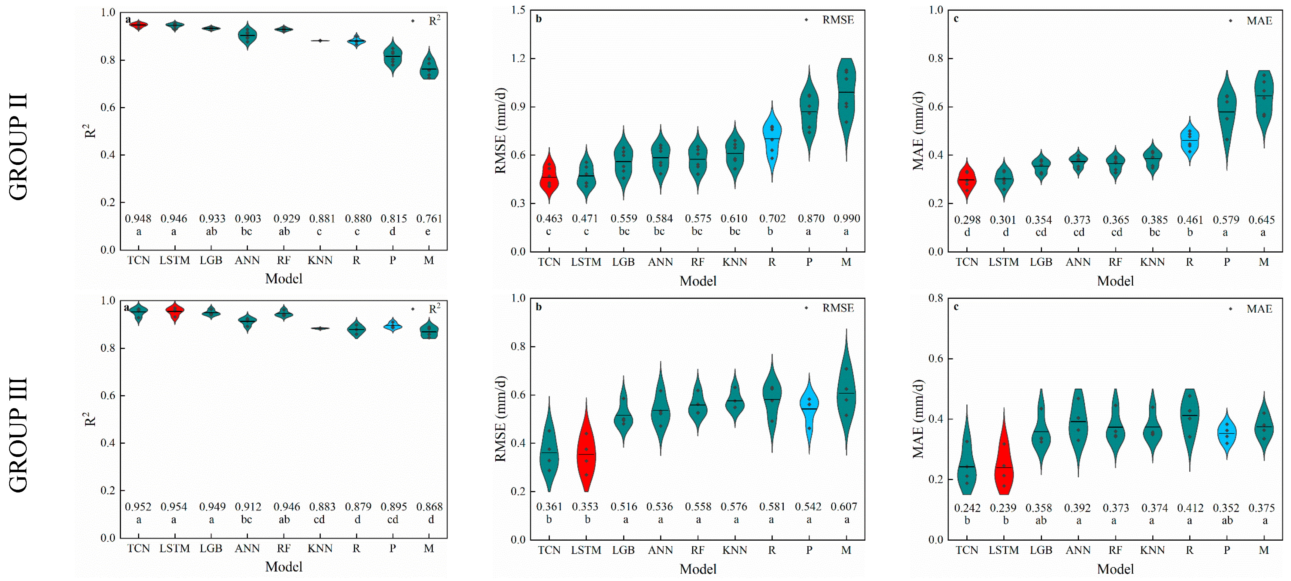
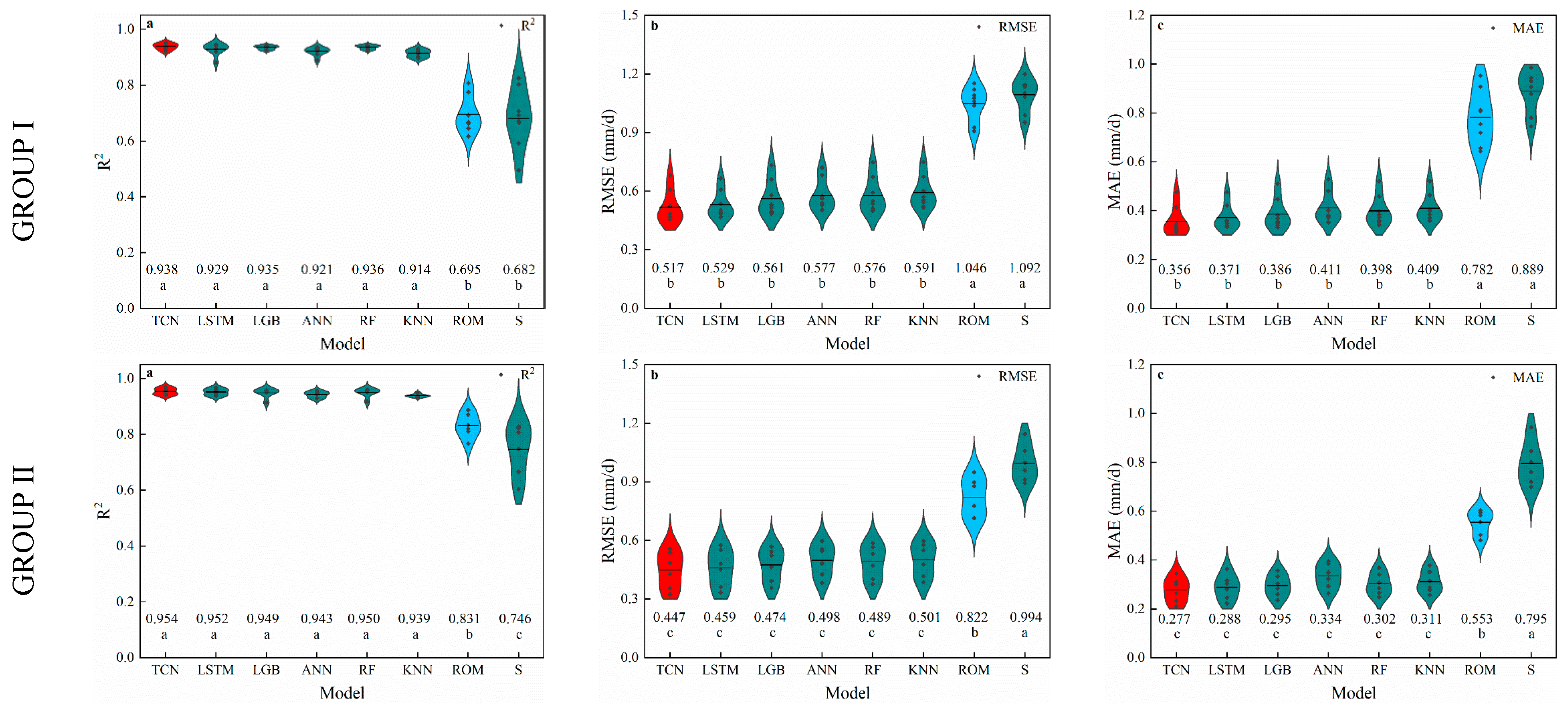
3.2. Radiation-Based Models

As shown in Figure 5, the R models performed the best in the first group and the second group (with an R2 of 0.839, RMSE of 0.801 mm/d, and MAE of 0.561 mm/d for the first group, and an R2 of 0.880, RMSE of 0.702 mm/d and MAE of 0.461 mm/d for the second group, respectively) while the P model performed slightly better in the third group (with an R2 of 0.895, RRMSE of 0.542 mm/d, and MAE of 0.352). Thus, the prediction accuracies of TCN, LSTM, LGB, ANN, RF, and KNN, based on air temperature and radiation data, were compared with R in the first group and the second group, and with P in the third group.
Figure 5 shows that, in the first group, the R2 of the KNN and R models did not differ significantly, but the RMSE and MAE of KNN were lower than those of the R model. Figure 5 also illustrates that the TCN, LSTM, LGB, ANN, and RF all performed similarly better than the H model, with a significant increase in the mean R2 values ranging from 0.043 to 0.100, and a significant reduction in RMSE, 0.166–0.303 mm/d, and MAE, 0.118–0.214 mm/d, respectively. Additionally, TCN significantly outperformed ANN and slightly outperformed LSTM, LGB, and RF in terms of R2, as well as RMSE and MAE. It is clear, then, that the TCN model showed the highest R2 and lowest RMSE and MAE in the first group, as compared to other models. Similarly, the R2, RMSE, and MAE of the ANN, KNN, and R models did not differ significantly in the second group. Although the R2 and RMSE of the LSTM, LGB, RF, and R models did not differ significantly, the MAE was lower in the R model, indicating that the performance of the LSTM, LGB, and RF models was slightly better than that of the R model. Furthermore, the TCN model predicted ET0 with a higher R2 and a lower MAE than the R model, making it better than the R model in predicting ET0 based on radiation datasets. As for the third group, TCN, LSTM, LGB, ANN, RF, and KNN performed better than the P model according to the significant increase in the mean R2 values ranging from 0.045 to 0.074, and a significant reduction in RMSE, 0.158–0.244 mm/d, and MAE, 0.127–0.168 mm/d, respectively. According to these results, radiation-based machine learning models significantly outperformed radiation-based empirical models. Furthermore, compared with other machine learning models, TCN slightly increased in terms of R2 and decreased in terms of RMSE and MAE, indicating that the prediction accuracy of TCN presented the best results among the other machine learning models. Overall, in the first strategy, the TCN model showed better results in predicting ET0 based on radiation datasets.
As seen from Figure 6, the ET0 values predicted using the radiation-based machine learning models were closer to the ET0 values computed using the FAO-56 PM equation, demonstrating the satisfactory prediction accuracy of the proposed machine learning models. In particular, the TCN (with an R2 of 0.925, RMSE of 0.546 mm/d, and MAE of 0.385) performed comparably better than other machine learning models when calculating ET0. This demonstrated the TCN model’s excellent potential for ET0 prediction in the first group. For the second group, there was no discernible difference between the ANN and R models at the 0.05 probability level regarding the accuracy of calculating ET0 making use of radiation data, but the MAE of the ANN model was numerically greater than that of the R model. Figure 6 also illustrates that the TCN, LSTM, LGB, and RF models all performed similarly better than the R model, with a significant increase in the mean R2 values ranging from 0.049 to 0.068, and a significant reduction in RMSE, 0.127–0.239 mm/d, and MAE, 0.096–0.163 mm/d, respectively. Furthermore, the TCN model had the highest R2 (0.948), lowest RMSE (0.463 mm/d), and lowest MAE (0.298 mm/d), indicating that it was more accurate than LSTM, LGB, and RF in predicting ET0 in the second group. As for the third group, the ET0 values predicted by ANN, KNN, LGB, and RF were closer to those of the P model, demonstrating that these machine learning models have the same performance as empirical models in predicting ET0. The TCN and LSTM models were more accurate than the other machine learning and empirical models, according to R2, RMSE, and MAE performance criteria. Additionally, the LSTM model achieved the highest R2 (0.954), lowest RMSE (0.353 mm/d), and lowest MAE (0.239 mm/d). From the above results, it can be concluded that LSTM performed slightly better than TCN, LGB, and RF, and much better than the empirical models under the input combination of Tmax, Tmin, and Ra in the third group. In general, considering the overall prediction accuracy of the machine learning models under the combinations based on temperature and radiation data, the TCN model showed better results in terms of stability in the second strategy.

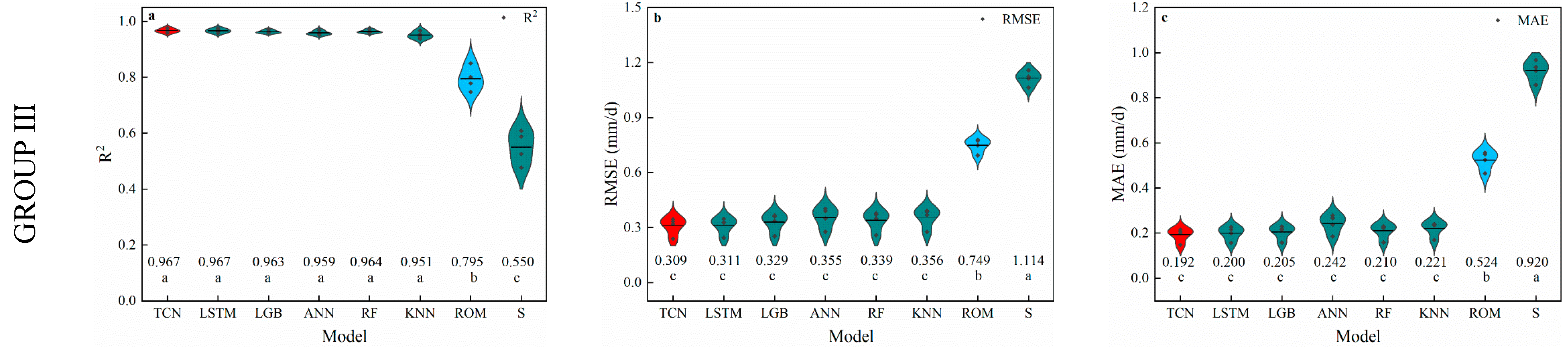
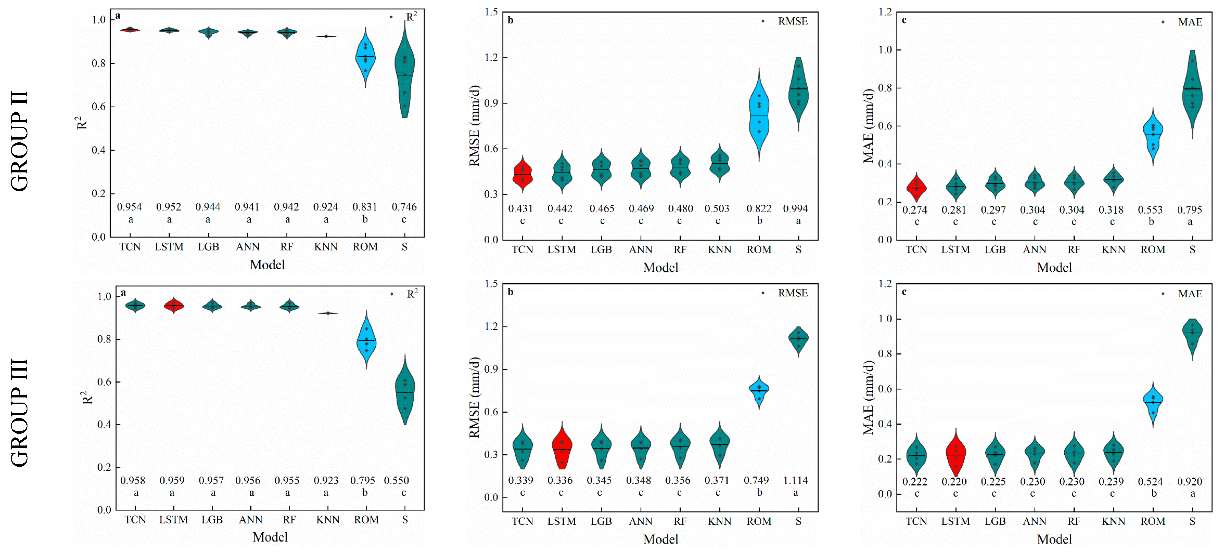
3.3. Humidity-Based Models

The mean R2, RMSE, and MAE of humidity-based machine learning and empirical models is summarized in Figure 7. According to Figure 7, the ROM model (with an R2 of 0.839, RMSE of 0.801 mm/d, and MAE of 0.561 mm/d) performed better than the S model in both strategies. Thus, the prediction accuracy of TCN, LSTM, LGB, ANN, RF, and KNN models, based on air temperature and humidity features, was compared with that of the ROM model.
For the first strategy, the R2 of the ROM was significantly lower than that of the machine learning models, and the RMSE and MAE of the ROM model were substantially higher than that of machine learning models, demonstrating that the machine learning models based on temperature and humidity data outperformed the empirical formulas. Furthermore, the R2 of TCN was slightly higher than that of other machine learning models, and the RMSE and MAE of TCN were slightly lower than those of other machine learning models, indicating that the performance of TCN was slightly better than the other machine learning models. In conclusion, all six of the machine learning models could outperform empirical equations in terms of accuracy, and the humidity-based TCN model outperformed the others.
For the second strategy (Figure 8), the R2 of the ROM model was significantly lower than that of machine learning models, and the RMSE and MAE of the ROM model were substantially higher than those of machine learning models, demonstrating that when it came to calculating ET0 outside of their training region, the machine learning models were well-trained and, based on humidity data, performed better than the empirical equations. In addition, the R2 of TCN (Group I and Group II) and LSTM (Group III) was slightly higher than that of the other machine learning models, and the RMSE and MAE of TCN (Group I and Group II) and LSTM (Group III) were slightly lower than those of other machine learning models, indicating that the performance of TCN (Group I and Group II) and LSTM (Group III) was slightly better than that of the other machine learning models. In conclusion, all six of the proposed machine learning models could outperform empirical equations in terms of accuracy, and the humidity-based TCN model outperformed the others in the first and second groups, while the humidity-based LSTM model outperformed the others in the third group.

4. Discussion

4.1. Performance of Temperature-Based Models

The Hargreaves method (H) was first proposed by Hargreaves and Samani for the estimation of ET0, and is commonly utilized around the world, as it only requires air temperature data as input and has a high accuracy [8]. Since the R2, RMSE, and MAE values of the ANN and KNN models were almost identical to those of the empirical models in all groups, we found that they had no effect on the accuracy of calculating ET0 in this investigation. The reason for this result might be that the layers of the ANN model were not too deep and the KNN model was relatively simple and did not require parameter estimation, resulting in a weak ability to capture nonlinear interactions between the weather and ET0, while Antonopoulos and Antonopoulos found that the temperature-based ANN has a larger R2 and lower MAE, outperforming the H equation [4]. Feng and Cui also reported that the ANN model outperforms the MH method [51]. There are two reasons for this opposite result. First, in general, lower values of MAE and RMSE or a higher R2 score cannot indicate a prediction closer to the actual value unless the low or high value is significantly smaller or larger, respectively. Second, there were significant regional differences in how well machine learning models predicted outcomes [27]. The prediction accuracy of TCN was noticeably superior to that of H or MH, despite the fact that LSTM, LGB, and RF did not perform noticeably better than H or MH in any group. Similarly, Chen et al., who stated that TCN presents the most accurate results based on air temperature data among six machine learning models, also came to the same conclusion [27].
Previous studies have mostly used data from the same station for training and testing models; we are thus unaware of their performance outside the research region. Some researchers have found a solution to this issue by grouping the meteorological data from every station, using this data set to build the training model, then testing each station independently [52]. In this study, all weather stations were located in Inner Mongolia in Northern China and were clustered into three groups using the K-means algorithm, and then, we tested the model developed by other stations in each group using one station within the groups. The meteorological data from each weather station were solely used for training or testing in this way. As a result, it was possible to acquire the model performance beyond the training weather station. In the three groups, the temperature-based TCN model outperformed the empirical method in terms of accuracy in predicting ET0.

4.2. Performance of Radiation-Based Models

Radiation-based empirical equations can obtain better ET0 estimation performance. According to several studies, temperature and radiation can account for approximately 80% of the fluctuation in ET0 [53]. In this research, three widely used empirical methods based on temperature and radiation data, namely, Makkink, Ritchie, and Priestley–Taylor, were selected for comparison with machine learning models [51]. The results showed that, under the combinations of temperature and radiation characteristics, all machine learning models were greatly outperformed by radiation-based empirical equations. Many studies have taken an interest in using machine learning models such as ANN, RF, and SVM to predict ET0 in recent years, with restricted meteorological features, and it has been discovered that their performance is superior to that of empirical equations [5,13]. Deep learning models, however, have been infrequently used to estimate ET0. Numerous research has demonstrated the superior performance of TCN, LSTM, and ANN in sequence problems. As a result, in this work, we modeled daily ET0 utilizing radiation data through these three deep learning models. According to the results, when radiation characteristics were provided, the RMSE and MAE of TCN were lower than those of KNN and ANN in Group I and slightly lower than those of the other machine learning models in general. This result might be due to the reasonable internal structure of TCN, which is more suited than other models to capturing the nonlinear interactions between weather and ET0.
In the second strategy, which involved training and testing the models in different weather stations, radiation-based machine learning models estimated ET0 with a significantly higher accuracy than empirical equations. This conclusion showed that, outside of the training set of weather stations, machine learning models based on radiation data outperform empirical models. It is noteworthy that in the second strategy, the TCN and LSTM outperform the other machine learning machine models.

4.3. Performance of Humidity-Based Models

The humidity-based ROM equation’s RMSE and MAE were lower in this investigation than those of the S equation, showing that ROM performed better than the S model overall. It is noteworthy that the ROM model’s performance was only marginally superior to that of the H and MH, while adding humidity data did not improve the prediction accuracy of the S model in estimating ET0, but further worsened its prediction performance. In contrast to the temperature-based equation, the empirical formula based on temperature and humidity data does not employ extraterrestrial radiation as an input, which might be the cause of this outcome. However, when RH was added as the input variable of the machine learning models, the estimation accuracy of ET0 was significantly improved compared to the temperature-based machine learning models. It is reasonable to give a machine learning model more features to generally improve its accuracy in predicting ET0.
All humidity-based machine learning models achieved a much greater accuracy in evaluating ET0 than humidity-based empirical models, similar to the results of the radiation-based machine learning models. It has been proven that the performance of the proposed machine learning models was also noticeably better than that of traditional methods at given temperatures and RH characteristics. It is worth noting that the TCN model outperformed all other proposed humidity-based machine learning models, having the highest R2, the lowest RMSE, and the lowest MAE. The causal and dilated convolutional layers of the TCN model’s internal structure, which have the ability to “remember” previous information, might be the cause of its superior performance.
In the second strategy, the proposed machine learning models all outperformed the empirical equations, which further proved that when predicting ET0 using humidity factors beyond the training region, applicable machine learning models can achieve a much greater level of accuracy. The findings demonstrated that, when the inputs of machine learning include humidity features, according to RMSE and MAE performance criteria, the TCN model was more accurate than other machine learning models in Groups I and II, and the LSTM model was more accurate than other machine learning models in Group III. It is worth mentioning that, most importantly, the proposed humidity-based machine learning model has a better performance, suggesting that, in the absence of local meteorological data, the proposed machine learning model could be built using cross-station data with similar meteorological characteristics to estimate the daily ET0 of the target station, which has scarcely been reported in previous studies.

5. Conclusions

In this study, six machine learning models were proposed for daily ET0 estimation under incomplete meteorological data in eastern Inner Mongolia, China. In addition, this study adopted two strategies to evaluate the ET0 prediction performance of the proposed machine learning models: (1) we trained and tested the proposed model separately in every single weather station, and (2), according to the average climate characteristics of eastern Inner Mongolia meteorological stations, they were divided into three groups using the K-means method. Then, each station in each group took turns serving as a validation station, testing the models trained by the other stations within the group. The results demonstrated that (1) in the three groups, the temperature-based TCN model outperformed the empirical method in the accuracy of predicting ET0 in the first strategy, and in the second strategy, temperature-based TCN, LSTM, and LGB models performed significantly or slightly better than the empirical method; (2) in both strategies, all radiation-based machine learning models provided more accurate results than the empirical methods, particularly the TCN model; and (3) in both strategies, all humidity-based machine learning models provided more accurate results than the empirical methods, particularly the TCN model. Most importantly, when only temperature characteristics were available, only the TCN model had an overall greater prediction accuracy than the empirical method based on the calibration temperature in both local and external areas. However, when the radiation or humidity characteristics were added to the given temperature characteristics, all the proposed machine learning models could estimate ET0, and their accuracy was higher than that of the calibrated empirical equations external to the training study area, which makes it possible to develop an ET0 estimation model for cross-station data with similar meteorological characteristics to obtain a satisfactory ET0 estimation for the target station.

Author Contributions

Conceptualization, H.Z.; methodology, H.Z. and J.X.; software, H.Z.; validation, J.X. and Z.L.; formal analysis, H.Z.; investigation, H.Z.; resources, J.X. and Z.L.; data curation, J.X.; writing—original draft preparation, H.Z.; writing—review and editing, J.M. and F.M.; visualization, H.Z.; supervision, J.M.; project administration, F.M.; funding acquisition, F.M. All authors have read and agreed to the published version of the manuscript.

Funding

This work was supported by the Earmarked Fund for China Agriculture Research System (CARS-02) and the National Key Research and Development Program of China (2017YFD0300801).

Data Availability Statement

The dataset used during this study can be obtained from the National Meteorological Information Center of China Meteorological Administration or from the corresponding author upon reasonable request.

Acknowledgments

We would like to thank the National Climatic Centre of the China Meteorological Administration for providing the climate database used in this study. This work was also supported by the Earmarked Fund for China Agriculture Research System (CARS-02) and the National Key Research and Development Program of China (2017YFD0300801).

Conflicts of Interest

The authors declare no conflict of interest.

References

  1. Kisi, O. Modeling reference evapotranspiration using three different heuristic regression approaches. Agric. Water Manage. 2016, 169, 162–172. [Google Scholar] [CrossRef]
  2. Shiri, J. Evaluation of FAO56-PM, empirical, semi-empirical and gene expression programming approaches for estimating daily reference evapotranspiration in hyper-arid regions of Iran. Agric. Water Manage. 2017, 188, 101–114. [Google Scholar] [CrossRef]
  3. Tabari, H.; Kisi, O.; Ezani, A.; Hosseinzadeh Talaee, P. SVM, ANFIS, regression and climate based models for reference evapotranspiration modeling using limited climatic data in a semi-arid highland environment. J. Hydrol. 2012, 444, 78–89. [Google Scholar] [CrossRef]
  4. Antonopoulos, V.Z.; Antonopoulos, A.V. Daily reference evapotranspiration estimates by artificial neural networks technique and empirical equations using limited input climate variables. Comput. Electron. Agric. 2017, 132, 86–96. [Google Scholar] [CrossRef]
  5. Feng, Y.; Cui, N.; Gong, D.; Zhang, Q.; Zhao, L. Evaluation of random forests and generalized regression neural networks for daily reference evapotranspiration modelling. Agric. Water Manage. 2017, 193, 163–173. [Google Scholar] [CrossRef]
  6. Ferreira, L.B.; da Cunha, F.F. New approach to estimate daily reference evapotranspiration based on hourly temperature and relative humidity using machine learning and deep learning. Agric. Water Manage. 2020, 234, 106113. [Google Scholar] [CrossRef]
  7. Abdullah, S.S.; Malek, M.A.; Abdullah, N.S.; Kisi, O.; Yap, K.S. Extreme Learning Machines: A new approach for prediction of reference evapotranspiration. J. Hydrol. 2015, 527, 184–195. [Google Scholar] [CrossRef]
  8. Hargreaves, G.H.; Samani, Z.A. Reference crop evapotranspiration from temperature. Appl. Eng. Agric. 1985, 1, 96–99. [Google Scholar] [CrossRef]
  9. Ahooghalandari, M.; Khiadani, M.; Jahromi, M.E. Developing equations for estimating reference evapotranspiration in Australia. Water Resour. Manage. 2016, 30, 3815–3828. [Google Scholar] [CrossRef]
  10. Priestley, C.H.B.; Taylor, R.J. On the assessment of surface heat flux and evaporation using large-scale parameters. Mon. Weather Rev. 1972, 100, 81–92. [Google Scholar] [CrossRef]
  11. Jones, J.; Ritchie, J. Crop growth models. In Management of Farm Irrigation Systems; Hoffman, G.J., Howell, T.A., Solomon, K.H., Eds.; ASAE: St. Joseph, MO, USA, 1990; pp. 63–89. [Google Scholar]
  12. Valiantzas, J.D. Simplified forms for the standardized FAO-56 Penman–Monteith reference evapotranspiration using limited weather data. J. Hydrol. 2013, 505, 13–23. [Google Scholar] [CrossRef]
  13. Ferreira, L.B.; da Cunha, F.F.; de Oliveira, R.A.; Fernandes Filho, E.I. Estimation of reference evapotranspiration in Brazil with limited meteorological data using ANN and SVM—A new approach. J. Hydrol. 2019, 572, 556–570. [Google Scholar] [CrossRef]
  14. Djaman, K.; Balde, A.B.; Sow, A.; Muller, B.; Irmak, S.; N’Diaye, M.K.; Manneh, B.; Moukoumbi, Y.D.; Futakuchi, K.; Saito, K. Evaluation of sixteen reference evapotranspiration methods under sahelian conditions in the Senegal River Valley. J. Hydol. Reg. Stud. 2015, 3, 139–159. [Google Scholar] [CrossRef]
  15. Valipour, M. Application of new mass transfer formulae for computation of evapotranspiration. J. Appl. Water Eng. Res. 2014, 2, 33–46. [Google Scholar] [CrossRef]
  16. Majhi, B.; Naidu, D.; Mishra, A.P.; Satapathy, S.C. Improved prediction of daily pan evaporation using Deep-LSTM model. Neural Comput. Appl. 2019, 32, 7823–7838. [Google Scholar] [CrossRef]
  17. Fan, J.; Yue, W.; Wu, L.; Zhang, F.; Cai, H.; Wang, X.; Lu, X.; Xiang, Y. Evaluation of SVM, ELM and four tree-based ensemble models for predicting daily reference evapotranspiration using limited meteorological data in different climates of China. Agric. For. Meteorol. 2018, 263, 225–241. [Google Scholar] [CrossRef]
  18. Mohammadi, B.; Mehdizadeh, S. Modeling daily reference evapotranspiration via a novel approach based on support vector regression coupled with whale optimization algorithm. Agric. Water Manage. 2020, 237, 106145. [Google Scholar] [CrossRef]
  19. Chia, M.Y.; Huang, Y.F.; Koo, C.H. Support vector machine enhanced empirical reference evapotranspiration estimation with limited meteorological parameters. Comput. Electron. Agric. 2020, 175, 105577. [Google Scholar] [CrossRef]
  20. Wen, X.; Si, J.; He, Z.; Wu, J.; Shao, H.; Yu, H. Support-Vector-Machine-Based Models for Modeling Daily Reference Evapotranspiration With Limited Climatic Data in Extreme Arid Regions. Water Resour. Manage. 2015, 29, 3195–3209. [Google Scholar] [CrossRef]
  21. Shiri, J. Improving the performance of the mass transfer-based reference evapotranspiration estimation approaches through a coupled wavelet-random forest methodology. J. Hydrol. 2018, 561, 737–750. [Google Scholar] [CrossRef]
  22. Rahimikhoob, A. Comparison between M5 Model Tree and Neural Networks for Estimating Reference Evapotranspiration in an Arid Environment. Water Resour. Manage. 2014, 28, 657–669. [Google Scholar] [CrossRef]
  23. Kisi, O.; Kilic, Y. An investigation on generalization ability of artificial neural networks and M5 model tree in modeling reference evapotranspiration. Theor. Appl. Climatol. 2015, 126, 413–425. [Google Scholar] [CrossRef]
  24. Yan, S.; Wu, L.; Fan, J.; Zhang, F.; Zou, Y.; Wu, Y. A novel hybrid WOA-XGB model for estimating daily reference evapotranspiration using local and external meteorological data: Applications in arid and humid regions of China. Agric. Water Manage. 2021, 244, 106594. [Google Scholar] [CrossRef]
  25. Maroufpoor, S.; Bozorg-Haddad, O.; Maroufpoor, E. Reference evapotranspiration estimating based on optimal input combination and hybrid artificial intelligent model: Hybridization of artificial neural network with grey wolf optimizer algorithm. J. Hydrol. 2020, 588, 125060. [Google Scholar] [CrossRef]
  26. Patil, A.P.; Deka, P.C. An extreme learning machine approach for modeling evapotranspiration using extrinsic inputs. Comput. Electron. Agric. 2016, 121, 385–392. [Google Scholar] [CrossRef]
  27. Chen, Z.; Zhu, Z.; Jiang, H.; Sun, S. Estimating daily reference evapotranspiration based on limited meteorological data using deep learning and classical machine learning methods. J. Hydrol. 2020, 591, 125286. [Google Scholar] [CrossRef]
  28. Yin, J.; Deng, Z.; Ines, A.V.M.; Wu, J.; Rasu, E. Forecast of short-term daily reference evapotranspiration under limited meteorological variables using a hybrid bi-directional long short-term memory model (Bi-LSTM). Agric. Water Manage. 2020, 242, 106386. [Google Scholar] [CrossRef]
  29. Petković, B.; Petković, D.; Kuzman, B.; Milovančević, M.; Wakil, K.; Ho, L.S.; Jermsittiparsert, K. Neuro-fuzzy estimation of reference crop evapotranspiration by neuro fuzzy logic based on weather conditions. Comput. Electron. Agric. 2020, 173, 105358. [Google Scholar] [CrossRef]
  30. Shan, X.; Cui, N.; Cai, H.; Hu, X.; Zhao, L. Estimation of summer maize evapotranspiration using MARS model in the semi-arid region of northwest China. Comput. Electron. Agric. 2020, 174, 105495. [Google Scholar] [CrossRef]
  31. Mehdizadeh, S. Estimation of daily reference evapotranspiration (ETo) using artificial intelligence methods: Offering a new approach for lagged ETo data-based modeling. J. Hydrol. 2018, 559, 794–812. [Google Scholar] [CrossRef]
  32. Dou, X.; Yang, Y. Evapotranspiration estimation using four different machine learning approaches in different terrestrial ecosystems. Comput. Electron. Agric. 2018, 148, 95–106. [Google Scholar] [CrossRef]
  33. Feng, Y.; Peng, Y.; Cui, N.; Gong, D.; Zhang, K. Modeling reference evapotranspiration using extreme learning machine and generalized regression neural network only with temperature data. Comput. Electron. Agric. 2017, 136, 71–78. [Google Scholar] [CrossRef]
  34. Karbasi, M. Forecasting of Multi-Step Ahead Reference Evapotranspiration Using Wavelet- Gaussian Process Regression Model. Water Resour. Manage. 2018, 32, 1035–1052. [Google Scholar] [CrossRef]
  35. Trajkovic, S. Hargreaves versus Penman-Monteith under Humid Conditions. J. Irrig. Drain. Eng. 2007, 133, 38–42. [Google Scholar] [CrossRef]
  36. Dorji, U.; Olesen, J.E.; Seidenkrantz, M.S. Water balance in the complex mountainous terrain of Bhutan and linkages to land use. J. Hydol. Reg. Stud. 2016, 7, 55–68. [Google Scholar] [CrossRef]
  37. Makkink, G.F. Testing the Penman Formula by Means of Lysimeters. J. Inst. Water Eng. 1957, 11, 277–288. [Google Scholar]
  38. Citakoglu, H.; Cobaner, M.; Haktanir, T.; Kisi, O. Estimation of monthly mean reference evapotranspiration in Turkey. Water Resour. Manage. 2014, 28, 99–113. [Google Scholar] [CrossRef]
  39. Allen, R.; Pereira, L.; Raes, D.; Smith, M.; Allen, R.G.; Pereira, L.S.; Martin, S. Crop Evapotranspiration: Guidelines for Computing Crop Water Requirements; FAO: Rome, Italy, 1998. [Google Scholar]
  40. Breiman, L. Random Forests. Mach. Learn. 2001, 45, 5–32. [Google Scholar] [CrossRef]
  41. Earnest, A.; Tan, S.B.; Wilder-Smith, A. Meteorological factors and El Niño Southern Oscillation are independently associated with dengue infections. Epidemiol. Infect. 2012, 140, 1244–1251. [Google Scholar] [CrossRef]
  42. Kohli, S.; Godwin, G.T.; Urolagin, S. Sales Prediction Using Linear and KNN Regression. In Proceedings of the Advances in Machine Learning and Computational Intelligence, Singapore, 6–7 April 2019; pp. 321–329. [Google Scholar]
  43. Shah, K.; Patel, H.; Sanghvi, D.; Shah, M. A Comparative Analysis of Logistic Regression, Random Forest and KNN Models for the Text Classification. Augment. Hum. Res. 2020, 5, 12. [Google Scholar] [CrossRef]
  44. Lee, T.; Ouarda, T.B.M.J.; Yoon, S. KNN-based local linear regression for the analysis and simulation of low flow extremes under climatic influence. Clim. Dyn. 2017, 49, 3493–3511. [Google Scholar] [CrossRef]
  45. Ke, G.; Meng, Q.; Finley, T.; Wang, T.; Chen, W.; Ma, W.; Ye, Q.; Liu, T.-Y. LightGBM: A highly efficient gradient boosting decision tree. In Proceedings of the 31st International Conference on Neural Information Processing Systems, Long Beach, CA, USA, 4–9 December 2017; pp. 3149–3157. [Google Scholar]
  46. Cai, J.; Li, X.; Tan, Z.; Peng, S. An assembly-level neutronic calculation method based on LightGBM algorithm. Ann. Nucl. Energy 2021, 150, 107871. [Google Scholar] [CrossRef]
  47. Yu, Q.; Guan, X.; Zhai, Y.; Meng, Z. The missing data filling method of the industrial internet platform based on rules and lightGBM. IFAC-PapersOnLine 2020, 53, 152–157. [Google Scholar] [CrossRef]
  48. Sun, X.; Liu, M.; Sima, Z. A novel cryptocurrency price trend forecasting model based on LightGBM. Financ. Res. Lett. 2020, 32, 101084. [Google Scholar] [CrossRef]
  49. Hochreiter, S.; Schmidhuber, J. Long Short-Term Memory. Neural Comput. 1997, 9, 1735–1780. [Google Scholar] [CrossRef]
  50. Lea, C.; Flynn, M.D.; Vidal, R.; Reiter, A.; Hager, G.D. Temporal Convolutional Networks for Action Segmentation and Detection. In Proceedings of the 2017 IEEE Conference on Computer Vision and Pattern Recognition (CVPR), Honolulu, Hawaii, USA, 21–26 July 2017; pp. 1003–1012. [Google Scholar]
  51. Feng, Y.; Cui, N.; Zhao, L.; Hu, X.; Gong, D. Comparison of ELM, GANN, WNN and empirical models for estimating reference evapotranspiration in humid region of Southwest China. J. Hydrol. 2016, 536, 376–383. [Google Scholar] [CrossRef]
  52. Reis, M.M.; da Silva, A.J.; Zullo Junior, J.; Tuffi Santos, L.D.; Azevedo, A.M.; Lopes, É.M.G. Empirical and learning machine approaches to estimating reference evapotranspiration based on temperature data. Comput. Electron. Agric. 2019, 165, 104937. [Google Scholar] [CrossRef]
  53. Samani, Z. Estimating solar radiation and evapotranspiration using minimum climatological data. J. Irrig. Drain. Eng. 2000, 126, 265–267. [Google Scholar] [CrossRef]
Figure 1. Spatial distribution of the weather stations.
Water 14 02890 g001
Figure 2. Number of clusters for K-means using the silhouette coefficient.
Water 14 02890 g002
Figure 3. The performance of the temperature-based models during the first strategy: (a) determination coefficient (R2), (b) root mean square error (RMSE), and (c) mean absolute error (MAE). Note: Values on the same line with different lowercase letters are significantly different at the 5% probability level. The same is shown below.
Water 14 02890 g003
Figure 4. The performance of the temperature-based models during the second strategy: (a) determination coefficient (R2), (b) root mean square error (RMSE), and (c) mean absolute error (MAE).
Water 14 02890 g004
Figure 5. The performance of the radiation-based models during the first strategy: (a) determination coefficient (R2), (b) root mean square error (RMSE), and (c) mean absolute error (MAE).
Water 14 02890 g005
Figure 6. The performance of the radiation-based models during the second strategy: (a) determination coefficient (R2), (b) root mean square error (RMSE), and (c) mean absolute error (MAE).
Water 14 02890 g006aWater 14 02890 g006b
Figure 7. The performance of the humidity-based models during the first strategy: (a) determination coefficient (R2), (b) root mean square error (RMSE), and (c) mean absolute error (MAE).
Water 14 02890 g007aWater 14 02890 g007b
Figure 8. The performance of the humidity-based models during the second strategy: (a) determination coefficient (R2), (b) root mean square error (RMSE), and (c) mean absolute error (MAE).
Water 14 02890 g008aWater 14 02890 g008b
Table 1. Geographic and meteorological information of the 18 weather stations and the cluster number of weather stations during the period 1960–2019.
StationU2
(m·s−1)
RH
(%)
SH
(h)
Tmin
(°C)
Tmax
(°C)
p
(mm)
Cluster
Eergunaqi2.0666.417.26−8.664.611.123
Tulihe2.0870.796.93−12.454.361.423
Manzhouli3.9962.038.08−6.976.350.902
Hailaer3.2266.127.39−6.675.551.092
Xiaoergou1.5666.257.31−7.318.391.573
Xinbaerhuyouqi3.7659.398.35−4.437.820.732
Xinbaerhuzuoqi3.2762.167.97−5.126.800.892
Zhalantun2.6856.647.58−2.189.661.552
Aershan2.4968.647.15−9.304.841.503
Suolun2.8256.827.74−3.8810.381.402
Zhaluteqi2.7048.237.901.2713.281.131
Balinzuoqi2.6650.028.31−1.0412.921.111
Linxi2.8349.588.09−1.2511.601.101
Kailu3.8351.808.480.8513.440.981
Tongliao3.5654.348.181.2413.291.121
Wengniuteqi2.9547.698.200.4113.031.051
Chifeng2.4248.178.011.5414.471.101
Baoguotu3.2349.947.991.5913.711.231
Note: the numbers 1, 2, and 3 under “cluster” indicate that the meteorological stations belong to clusters 1, 2, and 3, respectively. U2, RH, SH, Tmax, Tmin, and P are the average daily wind speed at 2 m height, relative humidity, sunshine duration, maximum and minimum air temperature, respectively.
Publisher’s Note: MDPI stays neutral with regard to jurisdictional claims in published maps and institutional affiliations.

