
Assessing Riverbed Surface Destabilization Risk Downstream Isolated Vegetation Elements
by
 , , ,
, , ,
Yi Xu
1,*,
Manousos Valyrakis
1,*,
Gordon Gilja
2 ,
,
Panagiotis Michalis
3,4 ,
,
Oral Yagci
5 and
Łukasz Przyborowski
6 1
School of Engineering, University of Glasgow, Glasgow G12 8LT, UK
2
Department of Hydroscience and Engineering, Faculty of Civil Engineering, University of Zagreb, HR-10000 Zagreb, Croatia
3
School of Civil Engineering, National Technical University of Athens, 15773 Athens, Greece
4
Research and Innovation Department, INNOVATEQUE, 15561 Athens, Greece
5
Civil Engineering Faculty, Division of Hydraulics, School of Engineering, Istanbul Technical University, Istanbul 34469, Turkey
6
Institute of Geophysics, Polish Academy of Sciences, 01-452 Warsaw, Poland
*
Authors to whom correspondence should be addressed.
Water 2022, 14(18), 2880; https://doi.org/10.3390/w14182880
Submission received: 27 July 2022
/
Revised: 27 August 2022
/
Accepted: 2 September 2022
/
Published: 15 September 2022
(This article belongs to the Section New Sensors, New Technologies and Machine Learning in Water Sciences)
Abstract
:A few decades ago, river erosion protective approaches were widely implemented, such as straightening the river course, enhancing riverbed/bank stability with layers of concrete or riprap, and increasing channel conveyance capacity (i.e., overwidening). However, recent research has established that such practices can be tremendously costly and adversely affect the rivers’ ecological health. To alleviate these effects, green river restoration has emerged as a sustainable and environmentally friendly approach that can reduce the negative impact of the riverbed and bank destabilization and flooding. One of the typical green restoration measures, especially for instream habitat improvement, is the establishment of instream vegetation, which leads to a more diversified flow regime, increasing habitat availability and serving as refugia for aquatic species. Within the perspective presented above, flow–vegetation interaction problems for several decades received significant attention. In these studies, rigid rods have commonly been used to simulate these vegetative roughness elements without directly assessing the riverbed destabilization potential. Here, an experimental study is carried out to investigate the effect of different instream vegetation porosity on the near-bed flow hydrodynamics and riverbed destabilization potential for a range of simulated vegetation species. Specifically, the flow field downstream, four distinct simulated vegetation elements is recorded using an acoustic Doppler velocimetry (ADV), assuming about the same solid volume fraction for the different vegetation elements. In addition, bed destabilization potential is assessed by recording with optical means (a He-Ne laser with a camera system) the entrainment rate of a 15 mm particle resting on the uniform bed surface and the number of impulses above a critical value. Results revealed that the number of impulses above a critical value at the normalized distance equal to two is a good indicator for cylinder and five for other vegetation to assess the riverbed destabilization potential. The experimental findings from this study have interesting geomorphological implications regarding the destabilization of the riverbed surface (removal of coarse particles induced by high magnitude turbulent impulses) and the successful establishment of seedlings downstream of instream vegetation.
1. Introduction
1.1. Parameters for Sediment Movement
Instream vegetation is significant for preserving rivers’ ecological health (providing safe refuge for fish habitats) but also protecting riverbed stability, which is considered the main challenge for critical infrastructure systems [1,2,3]. Recent climate change projections also highlight that extreme weather events are expected to increase in number [2]. This will add significant stress to riverine systems due to incidents associated with extreme flooding events leading to evolving erosive processes [4]. For instream vegetation in the riverbed channel, obstacle-induced turbulence in the vicinity of vegetation could initiate particle movement that could potentially affect the fluvial geomorphology and the bank stability [5,6]. In fluvial hydraulics, modeling flow fields and sediment entrainment rate in the presence of vegetation remains one of the most complex problems [7,8]. Therefore, deeply understanding the role of vegetation on sediment movement is highly critical in terms of its effect on streambank stability and riverbed morphology. In recent years, submerged vegetation in open channels has been extensively researched regarding its effect on flow resistance [9,10,11,12], which is one of the main reasons for resisting sediment entrainment.
The complex processes of flow field modification downstream vegetation elements, and whether different vegetation characteristics promote or demote the potential of bed surface destabilization have been explored by a plethora of research studies also using data-driven methods [13,14,15], in the last two decades. For flows through rigid vegetation patches, transport of bed surface material increases with generally increasing boundary shear stresses due to higher instream vegetation density [16,17,18,19,20,21]. Scour/deposition patterns on the riverbed, which is the responsible process for the expansion of instream patches, are mainly controlled by secondary flow and turbulence events generated around the plants [22,23]. For flows through instream vegetation, shear stresses near the riverbed have generally been considered as a key factor affecting riverbed surface stability. However, using boundary shear stresses to quantify sediment entrainment, is highly uncertain for open channel flows and practically fails for more complex flows such as around aquatic or riparian vegetation [21,24,25]. The shear flow velocity has been historically related to the boundary shear stress [26] in studying the effect of near-bed surface flow hydrodynamics on sediment entrainment. Many studies have been conducted by researchers to investigate the interaction between the particle movement and flow structures, such as mean flow velocity [27], and turbulence intensity [28] downstream vegetation elements. The density of vegetation (for both emergent and submerged vegetation) has been researched regarding removing its effect on the riverbed stability [29]. More recent research supports that turbulent kinetic energy is another relevant metric for studying sediment motions starting around instream vegetation [30,31].
Destabilization of the bed surface is a particle scale process that happens due to the combined strength of the mean and turbulent flow field downstream an obstacle to the flow, such as instream vegetation. The interaction of instream vegetation with the flow field including the generation of vortices shed downstream of it, and the complex ways this may lead to enhancing the risk of bed surface destabilization, are of strong interest to study. The possibility of particle movement varies with the magnitude of coherent flow structures and vortices acting on particles resting on the bed surface (filled black circle), as shown in Figure 1. Following the advection of a high magnitude flow structure, an exposed bed surface particle may get fully dislodged (dotted circle, Figure 1).
The criterion of critical bed shear stress gradually came into the researchers’ sight as a predictor of particle incipient motion in the vicinity of instream vegetation [32]. Some empirical equations based on near-bed velocity have been developed for bed shear stress calculation carried out in laboratory and field conditions [33]. Ref. [34] suggested an equation for shear stress estimation based on mean bed material diameter () and grain size distribution. The estimation criterion called Shields diagram for initiation of sediment motion indication was first made by [26] by building a relationship between the non-dimensional shear stress and the boundary Reynolds number. Many researchers have widely employed the Shields diagram as the primary method for incipient motion assessment.
Nevertheless, subsequent researchers [35,36,37] suggested reconsidering the threshold value of shear stress since the collected experimental data resulted in a high degree of scattering on the Shields diagram. As a result, more criteria such as the critical stream power [38] and the critical discharge [39,40,41] are employed by researchers for incipient motion in experimental flow conditions. However, these researchers did not consider the influence of solid/flexible vegetation-induced turbulence and coherent structures on sediment movement. Therefore, how to best assess riverbed destabilization is not fully explored, and a research gap remains, especially when considering the complex interplay of coherent flow structures and resulting sediment entrainment downstream instream vegetation.
Previous studies of the particle’s initial movement from the riverbed, which discussed the time-averaged bed shear stress without the plants present, were demonstrated to be inaccurate with vegetation [21,42]. In addition, previous works have also studied the effectiveness of such indicators, such as: velocity fluctuations [43]; turbulence structures [42]; and vortices [44,45]. Ref. [46] elaborates that the force is another criterion for sediment movement study when the acting force on a particle is larger than the resisting force. However, recent research proved that in regions with vegetation, the turbulent kinetic energy (TKE) performs better than previously discussed indicators in the prediction of the incipient motion of [21,31,43,47,48,49]. Furthermore, recent studies in the literature [50,51] have shed more light on the crucial role of fluctuating hydrodynamic forces for sediment particle movement, while a new sediment entrainment criterion based on the impulse theory, has been presented as a more robust and reliable predictor [47] and thus warrants further investigation herein.
1.2. Sediment Motion around Porous Vegetation
Vegetation morphology potentially influences the riverbed and riverine stabilization systems in the river. Many researchers show that aquatic and instream vegetation protect the riverbed surface from destabilization via reinforcement through its root system [52,53,54]. Refs. [55,56] elaborated that the different density of vegetation affects flow structure. [57] concluded that a high density of submerged vegetation could markedly prevent sediment movement and can retain up to 80% of the number of particles downstream of the vegetation. In addition to the vegetation density, Refs. [58,59,60] studied the influence of different vegetation sizes, shapes, and heights on sediment entrainment. Ref. [56] stated that the working mechanism of vegetation on sediment entrainment comes from the induced drag forces in terms of the restrain of momentum exchange by the frontal surface area when river flow passes through the vegetation. Conversely, Ref. [61] demonstrated that the vegetation patch could cause a higher particle entrainment rate due to increasing turbulence intensities under the same velocity condition. Instream vegetation generates higher turbulence intensity compared with no vegetation conditions [61]. Furthermore, the increase in the solid volume fraction of the plant leads to stronger turbulence downstream of vegetation, thus increasing the particle entrainment rates [62]. In addition, a submerged patch of simulated vegetation has been studied regarding its relative impact on the extent of suspended sediment deposition with the aspects of vegetation element height and diameter [63] and channel velocity and stem-generated turbulence [64].
Previous methods for destabilization assessment based on the above-discussed parameters involve significant uncertainties emerging from the limitations of the phenomenological or empirical approaches they are based on, using surrogate flow parameters such as the mean flow or Shield’s shear stresses. In contrast, this research aims to study the riverbed destabilization downstream instream vegetation patches by considering the actual dynamic process of particle-scale entrainment due to coherent flow structures shed downstream of them, having sufficient energy to result in full coarse particle entrainment. The main objective herein is to employ a modern dynamical criterion for particle entrainment, such as the impulse criterion [47,65], which is hypothesized to be appropriate for parameterizing the strength of coherent flow structures in removing riverbed material past instream vegetation patches, as shown in Figure 1. Here, in addition to the above criterion, the robustness of an optical system based on a helium–neon (He-Ne) laser with a camera, is also explored for directly assessing the riverbed destabilization downstream of instream vegetation patches. This research presents a physically sound data driven approach based on the impulse criterion which is considering the conservation of momentum at a particle scale, where coherent flow structures downstream vegetation patches are sporadically (flow near threshold flow conditions) able to transfer enough momentum (via the flow impulses) towards the removal of coarse sediment particles.
2. Experimental Setup and Protocol
2.1. Experiment Setup
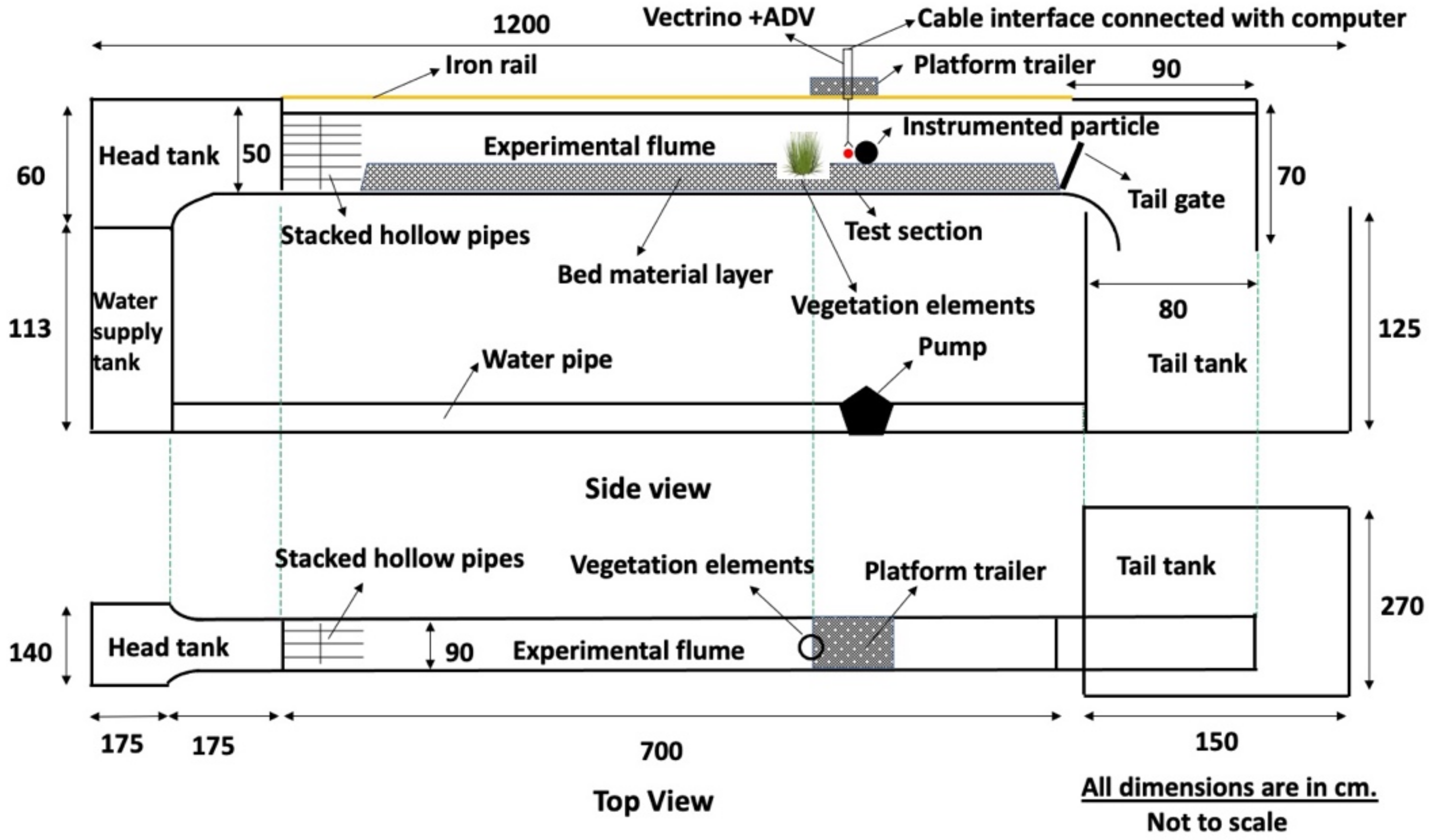
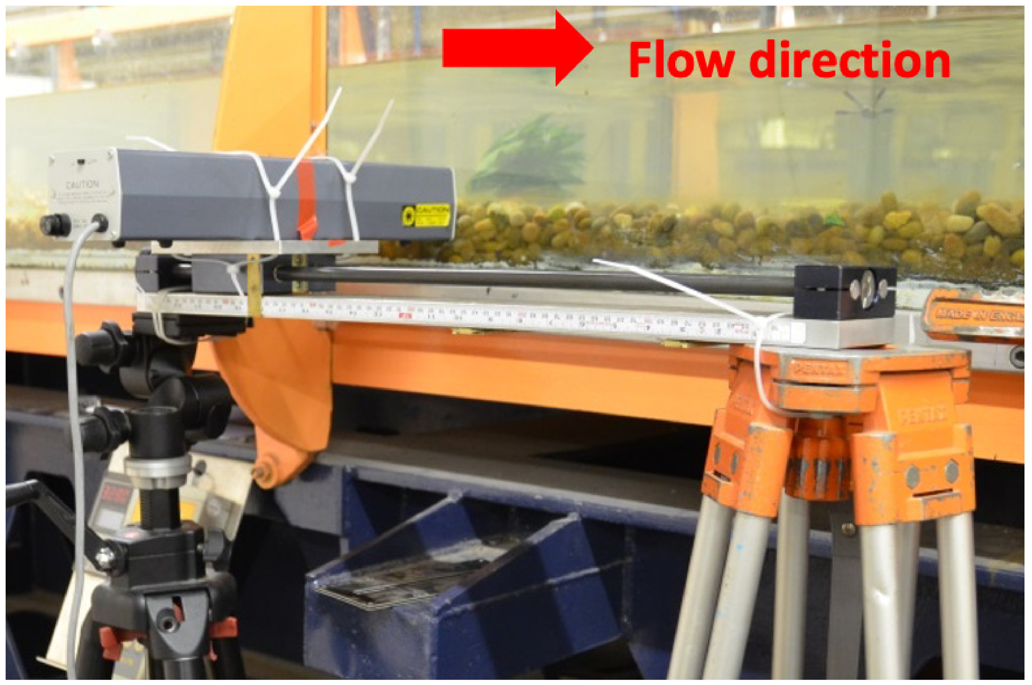
All experiments are carried out under uniform and steady flow conditions, at the main research flume of the hydraulic laboratory at the University of Glasgow, UK. The physical experiments are conducted in the water recirculating flume sized 90 cm wide and 12 m long, utilizing a 1.1 kW powered pump, which is capable of driving the water from the storage tank up to a flow rate of 3.6 m3/s. The flume has transparent glass on both sidewalls to facilitate visual observations and a steel frame to stabilize the entire flume. The experimental working section was located 525 cm downstream of the head tank and 175 cm upstream of the tailgate with a bed slope of 1/1000, where the flume bottom has a hydraulically smooth steel floor bed. The flume’s bottom was paved with vertically graded gravels (size increasing from bottom to top about 5 cm high) to achieve hydraulically rough flow conditions, and the flow depth was 13 cm at the test section. The platform trailer on the iron rail is designed to accommodate and position the acoustic Doppler velocimetry (ADV), as shown in Figure 2. The velocity profiles were taken utilizing the ADV when the steady flow conditions were achieved. Here, the He-Ne laser system with camera is also explored for assessing the riverbed destabilization downstream vegetation.
2.2. Vegetation Elements
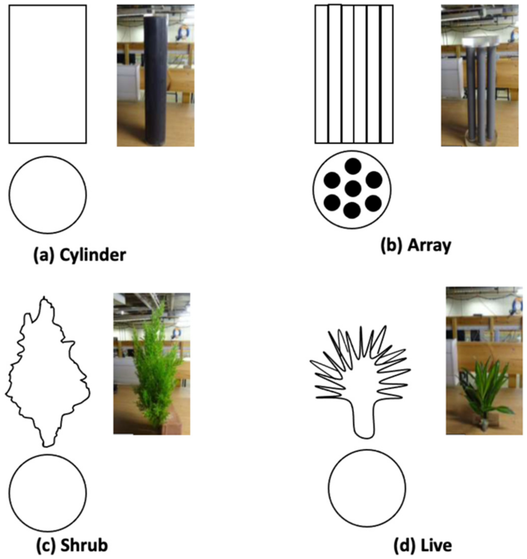
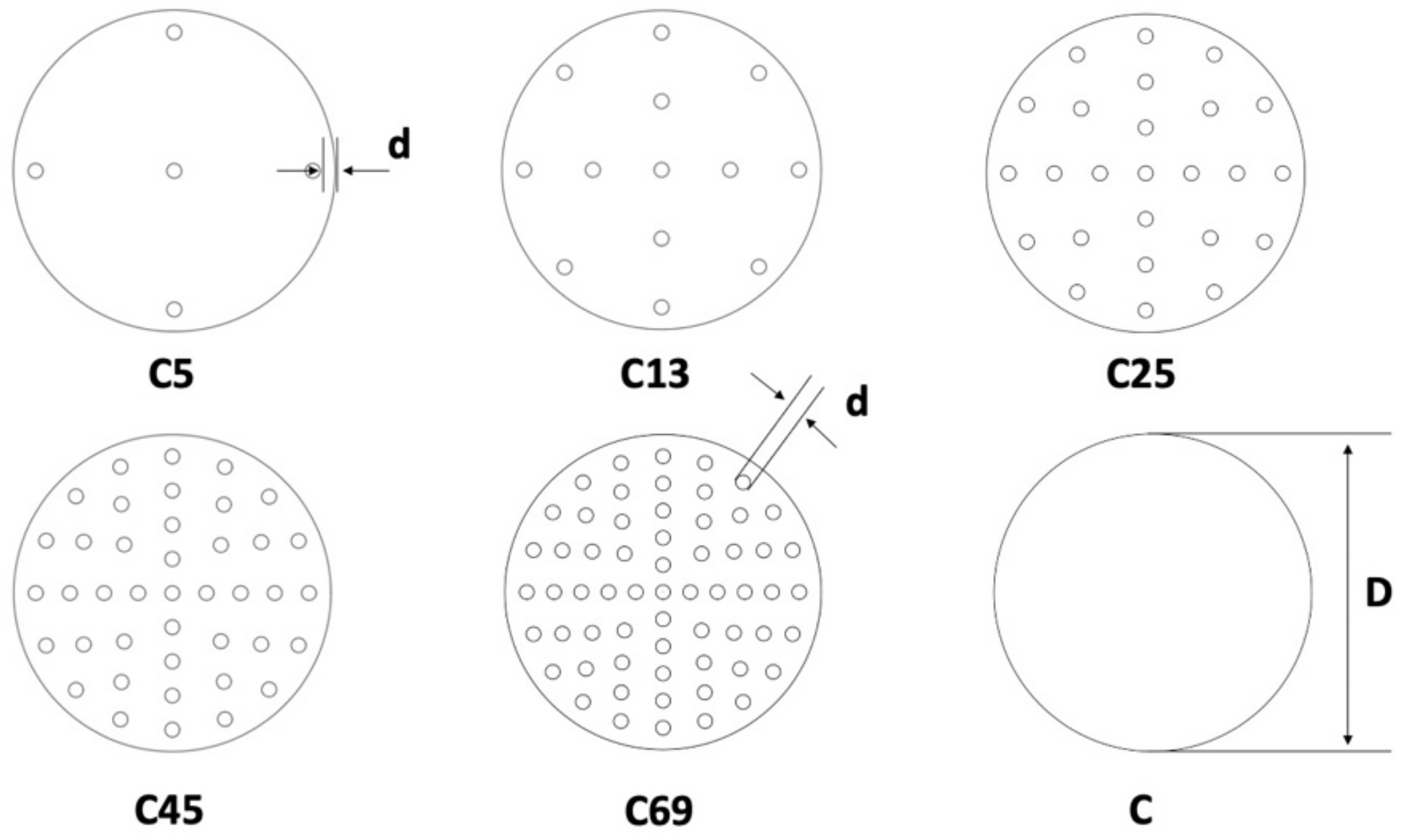
This experiment included two groups of model vegetation elements arranged inside circular areas with the same mean outer diameter of 110 mm. The criterion for selection of this diameter of vegetation was eliminating boundary effects with flume sidewalls. The first group included simulated vegetation patches comprising different numbers of rigid rods of 6 mm diameter achieving different densities, as shown in Figure 3b,c and Figure 4. The distinct porosity rigid vegetation elements are characterized by the number of rods within the patch—C5, C13, C25, C45, C69, and C—with corresponding densities of 1.25%, 3.15%, 6.25%, 11.25%, 17.25%, and 100%, respectively, as listed in Table 1. The volumetric ratio refers specifically to the solid volume ratio to the total volume. This group explores the particle entrainment downstream vegetation with rigid and high porosity characteristics. The second group includes four distinct vegetation types such as cylindrical elements, an array of small cylinders, plastic simulated shrubs, and patches of flexible live vegetation, as shown in Figure 3. It mainly focuses on the exploration of flexible and rigid porous vegetation. First, the flow measurements were taken by positioning the ADV along a grid of locations (seven distinct locations, each being one vegetation patch diameter apart downstream from the simulated vegetation patches) along the central line of the flume (Figure 2). Then, the particle measurements were completed, placing the particle at each distinct pocket downstream of the vegetation elements (corresponding to the distances about one diameter downstream from the element).
In Figure 3a, the solid cylinder represents the non-porous and rigid vegetation, such as tree trunks. The rigid hexagonal array of circular cylinders, may represent an array of tree trunks, reeds, or tree roots, as shown in Figure 3b. Shrub in Figure 3c represents the instream shrub without any bending during the tried flows. Finally, Figure 3d shows the live instream vegetation with flexible fronds representing the bending plant. The outer diameter for all the simulated vegetation elements was assumed to equal 10 cm. It is important to establish a clear porosity variation among these vegetation elements according to these vegetation characteristics ( , where , , , and represent the vegetation element porosity of cylinder, array, shrub, and live, respectively).
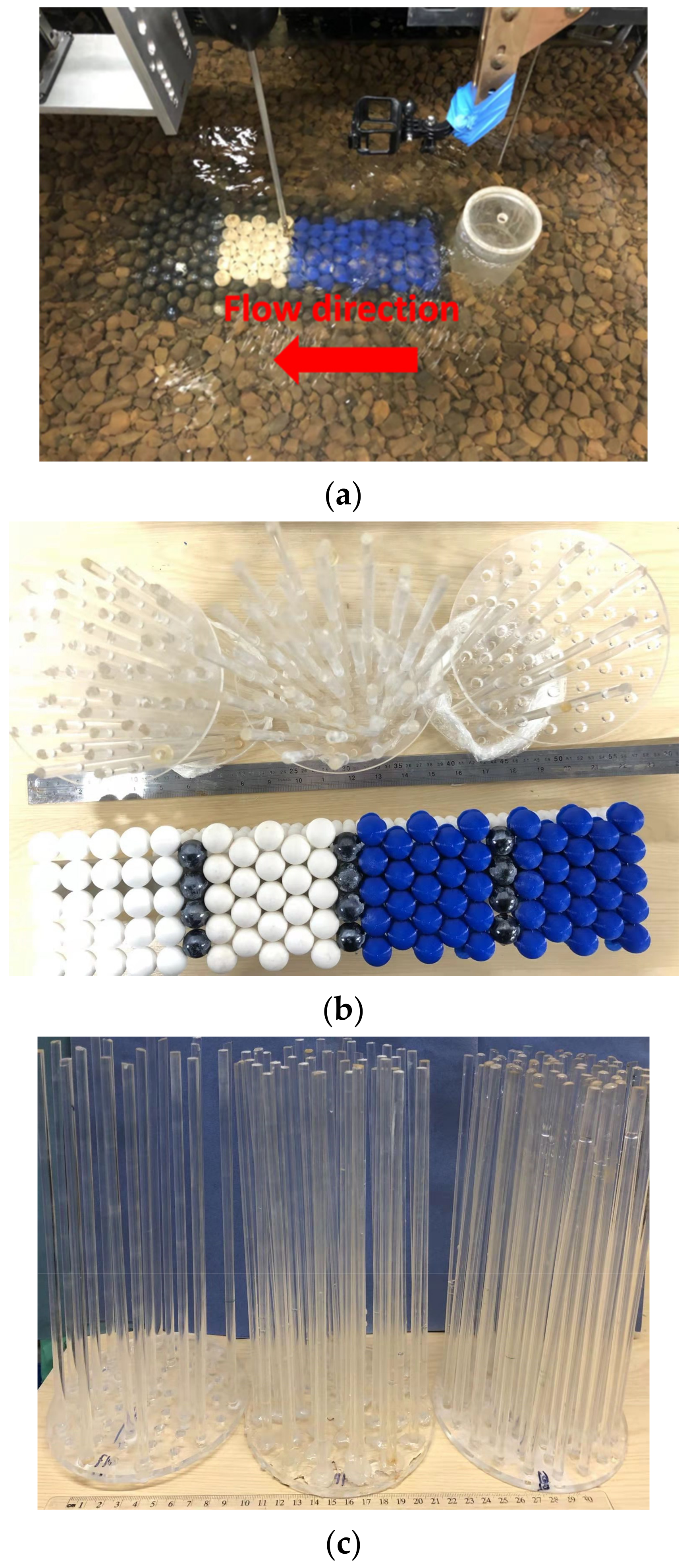
The number part in C5, C13, C25, C45, and C69 in Figure 4 denotes the number of rods installed in each patch. The C represents the full cylindrical pier model and d′ (=6 mm) indicates the distance from the edge of the patch to the nearest rod. Figure 5a is a picture of the test section with pier model, ADV and 3D printed layer. Figure 5b shows the vertical view of patches and the 3D printed spherical layer, and Figure 5c illustrates the side view of patches with different numbers of rods. The different porosity of instream vegetation is simulated by combining an artificially made patch (D = 120 mm) with a different number of solid rods (d = 6 mm), as shown in Figure 4 and Figure 5b,c.
The range of vegetation types and porosity is chosen to match the typical ranges assessed in the literature. For example, the types of vegetation shown in Figure 3 have been assessed by ([66]; see Table 1 therein) referred to as the solid cylinder (Figure 3a), hexagonal cylinder (Figure 3b), emergent vegetation (Figure 3c) and submerged vegetation (Figure 3d). For the case of simulated vegetation elements of distinct porosity, the choice of a range of the vegetation densities formed by the individual plastic rods (d = 0.006 m) is characteristic of very sparse to dense arrangements, similar to what is found in meadows or mangrove systems and natural marshes (including spartina species) [67].
2.3. Velocity Measurements
In high and low flow conditions, the matrix three-dimensional velocity profiles were recorded in seven longitudinal measurement points downstream vegetation elements using acoustic Doppler velocimetry (ADV) [68]. The ADV is vertically mounted on a moving platform capable of parallelly moving along the flume for recording the flow velocity for four minutes period at 25 Hz at an optimized configuration to minimize flow measurement uncertainties [69,70] sampling rate downstream of the vegetation with seven normalized distances. As the water flows through the ADV (Vectrino I©, Nortek, 1351 Rud, Norway) side-looking probe, the velocity will be instantaneously recorded at the measurement volume 5 cm upstream of it with a negligible effect on the flow field. The velocimetry recording duration is sufficiently long to allow reconstruction of the mean and turbulent flow velocity profiles.
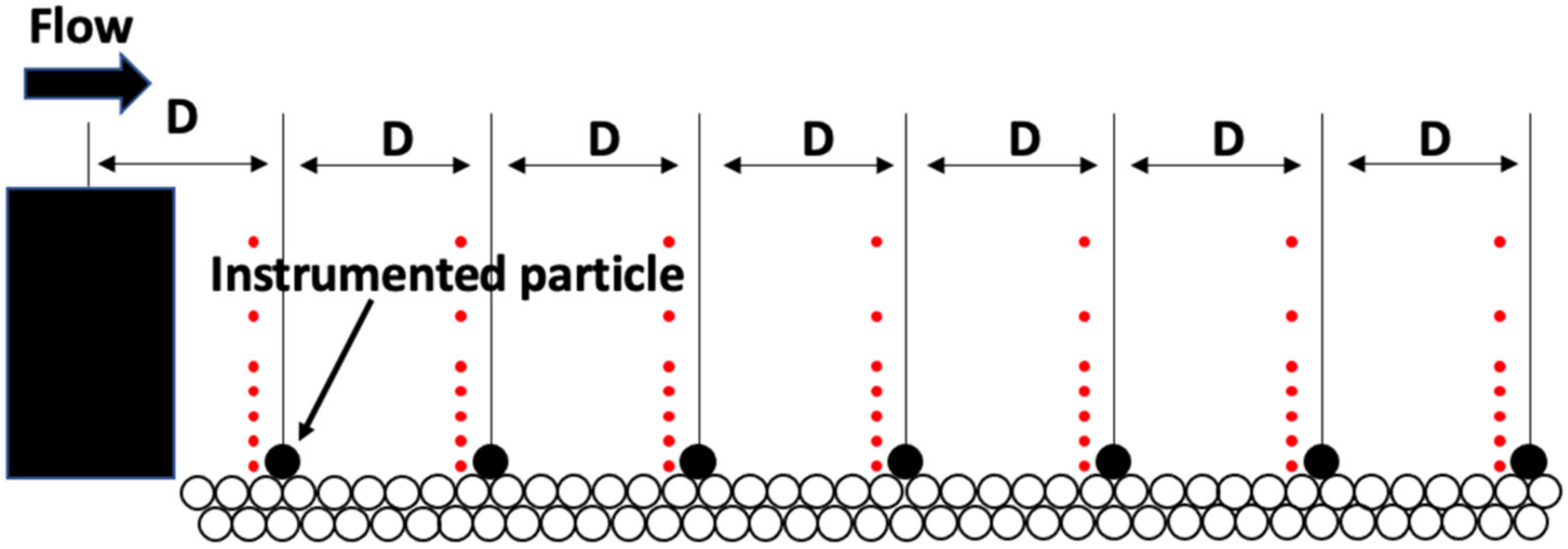
As shown in Figure 6, the test section is designed so that in all the experiments ADV measurements were performed in fixed positions, just upstream of each instrumented particle position: 3 mm, 6 mm, 12 mm, 20 mm, 30 mm, 55 mm, 80 mm, and 105 mm above the bed. The hydraulic conditions were kept the same between tests. The black cylinder represents the planted submerged vegetation elements with a designed diameter of D. As shown in Figure 3, the cylinder and array have a diameter of 110 mm while the shrub and live vegetation have an average diameter of 110 mm. To adequately characterize the variation of particle entrainment rate, an instrumented particle is adopted here and accurately positioned along the centerline of the seven longitudinal distances to visually read the number of movement times.
2.4. Instrumented Particle and Experimental Arrangement
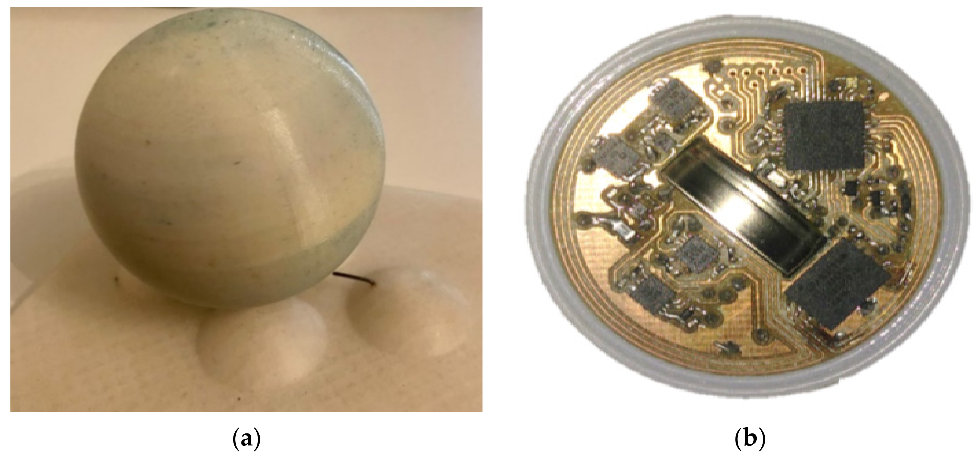
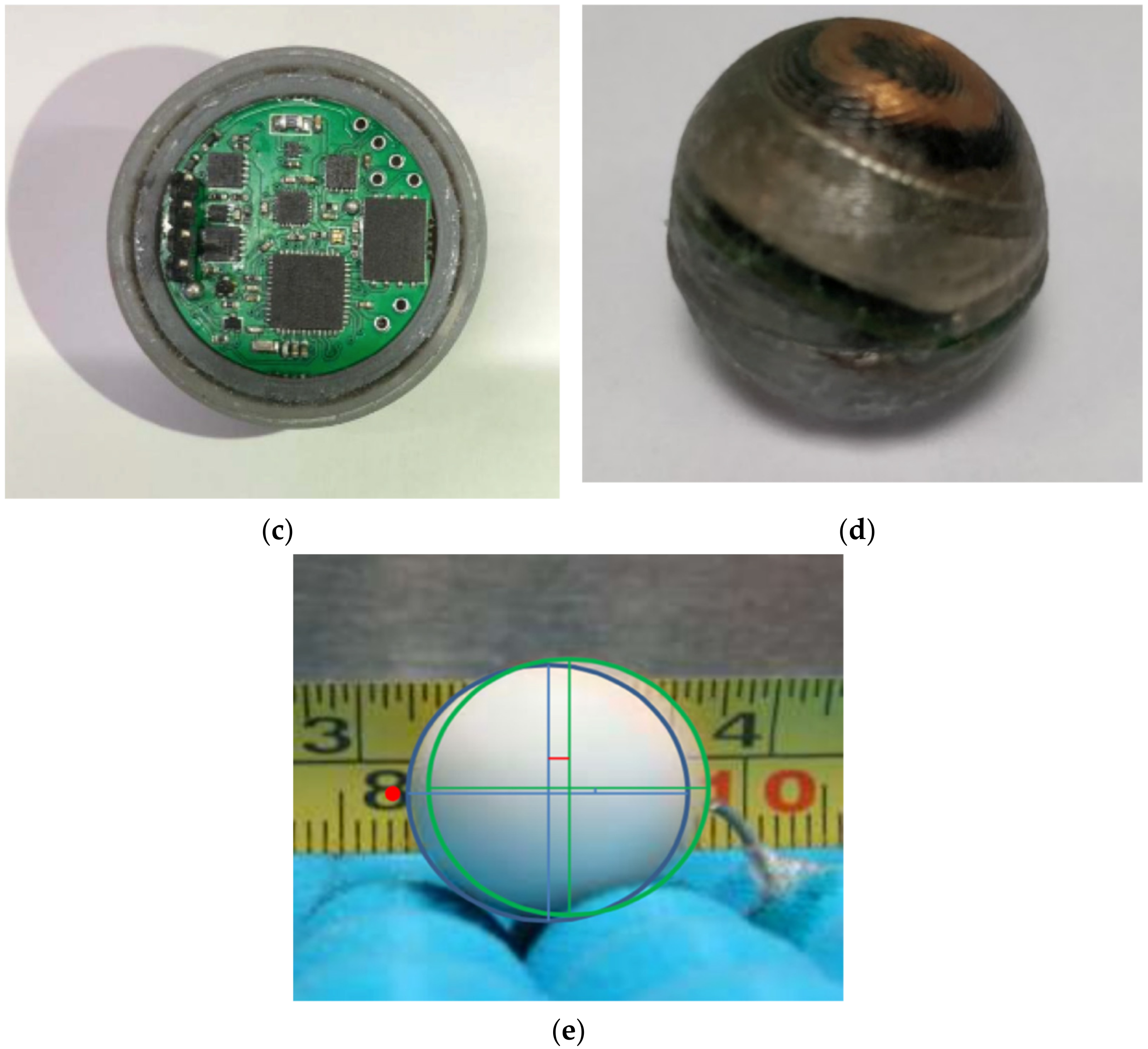
This section tests two groups of particles to monitor the riverbed destabilization potential downstream of the vegetation elements mentioned above. The first group includes three different sizes of instrumented particles with diameters of 30 mm, 40 mm, and 70 mm, and the second group is normal particles with a size of 15 mm and 20 mm, as shown in Figure 7. Particles with different particle sizes are used because there is no entrainment event when the particle diameter is tested from large to small until the particle with a diameter size of 15 mm is tested. Ref. [69] demonstrated the ability of instrumented particles to assess riverbed destabilization potential through the recorded particle entrainment. The entrainment rate of the novel instrumented particle is read through embedded microelectromechanical sensors (MEMS), which enable the recording of the particle’s three-dimensional displacement. Compared to past versions developed at our lab, this instrumented particle features miniaturized size and deployment improvements (including deployment time, waterproofing, and rugged shell). However, changes in any riverbed condition may potentially influence the entrainment of particles. Therefore, controlling the properties of this test section becomes extremely important. For this reason, a 3D printed riverbed layer was made by a diagonal array of hemispheres of the same diameter as the instrumented particle, as shown in Figure 7a,e. In addition, the pin behind the instrumented particle restricts its downstream entrainment by only allowing a 1.25 mm movement.
However, after several experimental test attempts for the particle entrainment with different sizes of instrumented particles, it was found that when these were placed downstream of the porous vegetation they did not move, for a wide range of combinations of sizes and densities allowed by the different instrumented particle designs, and for the range of flow conditions established. Therefore, the riverbed destabilization was then analyzed by direct observation of the entrainment of smaller (15 mm in diameter) and lighter test particles (Figure 7). Analysis was enhanced by the camera system capable of visually recording particle entrainment rates. Therefore, the first group of vegetation elements and the 15 mm test particle were used for the next analysis phase.
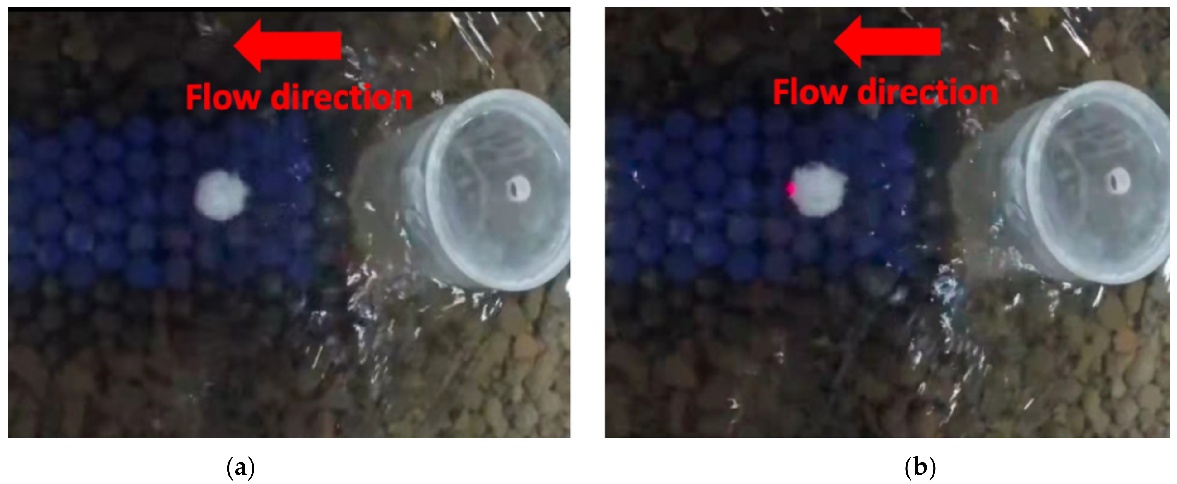
A digital video camera and a He-Ne laser system is employed here as an electric eye configuration to monitor the entrainment of the instrumented particles, as shown in Figure 8 and Figure 9. The He-Ne laser beam is set to partially target the exposed instrumented particle when resting on the test section of the bed surface, and the remainder of the beam is aimed at the camera. During full particle entrainments, the He-Ne laser beam is fully blocked, which is well captured by the digital camera, allowing to visually identify particle entrainment events and validate the entrainment rates recorded by the instrumented particle as shown in Figure 8a. Figure 8b illustrates the particle resting on its pocket of the 3D printed layer without any motion. The entrainment rate was calculated through blockage times of lights recorded through a camera with a recording rate of 29 frames/s. The occurrence of particle entrainment was manually reviewed through the video recorded by the camera within a 3 min duration. Each displacement event can be described as the particle blocking the light from the He-Ne laser once the particle leaves its original pocket, as illustrated in Figure 8. However, an obvious shortcoming of optical methods such as the He-Ne laser system is that it cannot accurately or with high resolution distinguish fine particle motions such as twitching and full entrainment. In contrast, the temporal resolution of the instrumented particles can be more substantial [69].
3. Results
Entrainments were observed only for the first group of vegetation analogs, referring to distinct instream vegetation categories of different porosity. The same group of vegetation elements (e.g., cylinder and array) is directly compared for the porosity at the same size. The data from these experiments were taken to analyze bed destabilization. Based on the experimental observations, no entrainment was observed for the second group of vegetation analogs, for all tried combinations of particle sizes and densities. Specifically, analysis of the sensor’s data showed that the instrumented particle recorded no entrainment events for all flume experiments under different porous elements of the second group due to the relatively low density of vegetation (the highest density of the patch was 17.25%, Table 1).
Thus, only the vegetation analogs from the first group of experiments, as shown in Figure 3, were used for the following analysis. Specifically, the flow properties downstream, distinct locations of each of the four vegetation elements of the first group are also linked to the test particle entrainment rates. The different porous characteristics for vegetation elements are therefore compared according to the measured entrainment rate, which potentially dictates the probability of riverbed destabilization.
These test results imply another possible reason for no entrainment of the larger particles: the rapidly fluctuating hydrodynamic forces acting around them (as tested here for the case of instrumented particles) are too short-lived, and to fully entrain them would require stronger fluctuations. So, the impulse criterion is also employed here as a theoretical model to assess the probability of entrainment events (parameterized using ADV recorded data). Meanwhile, to validate the reliability of this result, a smaller, non-instrumented particle with a diameter of 15 mm is employed here, accompanied by the He-Ne laser and camera system to observe the entrainment events.
3.1. Flow Structure in the Wake Region of Representative Vegetative Elements
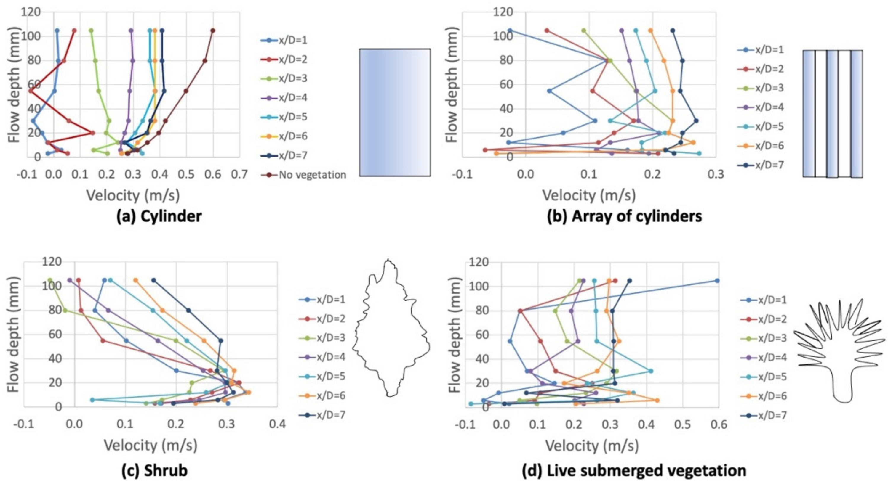
This section offers flow analysis results for the first group of vegetation patches. It can be seen that the mean flow velocities are dramatically varied with the distance downstream of the vegetation. In general, the velocity increases gradually along with the downstream of vegetation for all vegetation elements, as shown in Figure 10. However, near the riverbed, the velocity variation does not increase gradually but irregularly varies, especially for the array of cylinders, shrubs, and live vegetation. In this region near the bed, the presence of pronounced sub-canopy flow, which was demonstrated by [71,72] in a detailed manner, dominates the whole flow domain in the wake region. In addition, the shrub’s apparent variation tendency of velocity is displayed compared to other cases, where velocity sharply decreases when the flow depth is approximately higher than 20 mm, as shown in Figure 10c.
For most vegetation elements, the mean velocity deficit is more pronounced in the vicinity of the elements, with the mean flow gradually restoring to the mean ambient flow (assumed to be the “no vegetation” case) velocity profiles (see Figure 10a) from x/D = 1 to x/D = 7. Under the “no vegetation” case, velocities are higher than for all the cases with vegetation for flow depth higher than 20 mm. Specifically, for the shrub, the element’s geometry results in local flow accelerations below the canopy, which is persistent for a significant distance downstream of the vegetation elements (Figure 10c). The opposite happens to the submerged live vegetation, where local flow accelerations are relatively restricted near the bed surface, but more pronounced above the canopy and closer to the water surface (Figure 10d).
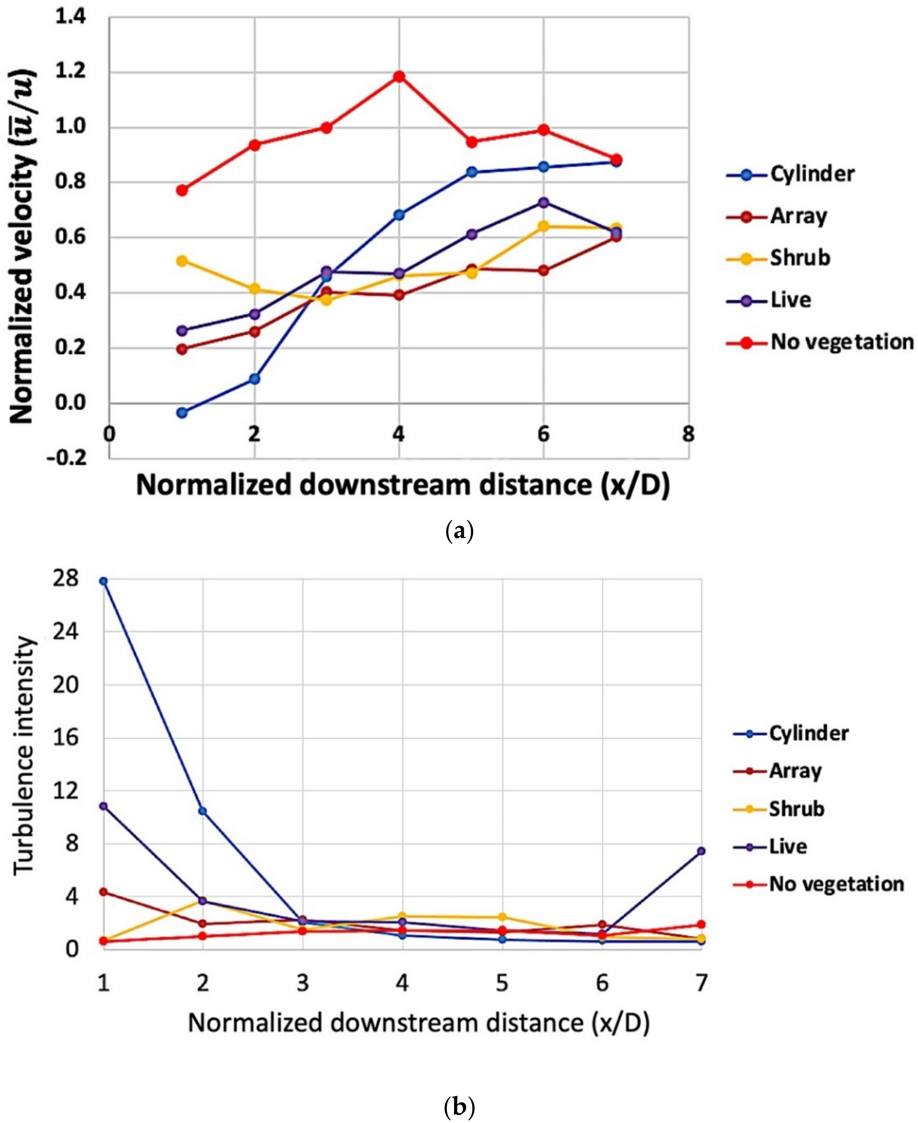
The existence of instream vegetation may increase the near-bed velocity and turbulence, according to the research studies by [19,66]. Figure 11 displays the variation of depth-averaged mean flow velocity and turbulence intensity at seven normalized isometric positions downstream for four vegetation elements. Compared to the depth-averaged mean flow velocity with no vegetation, all cases of vegetation have lower depth-averaged mean flow velocity, especially with decreasing distance from the vegetation. As expected, the value of depth-averaged mean flow velocity increases as the distance increases. It is worth mentioning that the lower porosity element (array) caused a higher velocity reduction due to weaker flow [72] and the higher resistance to the flow as shown in Figure 11a. Comparatively, the depth-averaged mean velocity for the array and live vegetation increases slowly as the flow progresses. Especially, the depth-averaged mean velocity downstream of the cylinder is markedly raised until the normalized distance reaches x/D = 5. As seen in Figure 11a, the depth-averaged mean flow velocity deficit is greater for the denser vegetation patches (cylinders and array of cylinders). While the depth-averaged mean flow velocity deficit is more pronounced in the vicinity of the rigid cylinder (Figure 11a), the mean velocity seems to restore faster for the cylinder compared to the other vegetation elements since the cylinder generates stronger later momentum transfer as previously demonstrated by [22].
As shown in Figure 11b, turbulence intensity increases with the introduction of any simulated vegetation element, relative to the case of no vegetation, but it sharply reduces with the downstream distances from them. Specifically, when the two rigid vegetation elements (cylinder and array) were compared, a higher volumetric ratio has lower velocity but much higher turbulence intensity in the nearest assessed location downstream of the obstacle. This was explained by [62] considering that lower permeability generates a more distinct shear layer and enhances the stronger lateral momentum exchange. Nevertheless, shrub and live vegetation elements have higher velocity than rigid cylinders just rear the body. As documented by [66], the highest turbulence intensity occurs just downstream of the vegetation element, and a gradually decreasing trend exists along the flow direction. Ref. [22] showed that the origin of the TKE is mainly due to lateral turbulence intensity and this effect mitigates with the decreasing solid volume fraction. Two things should be noticed here: the shrub’s highest turbulence intensity appears at x/D = 2, and the turbulence intensity suddenly sharp increases from the distance x/D = 6 to 7 of live vegetation. As discussed above, the turbulence intensity is controlled by the strength of bleed flow and adverse pressure gradient near the body, which depends on the porosity of vegetation. The turbulence intensity for live vegetation is higher than the array and shrub elements but with the highest porosity. Therefore, it can be elucidated that a more complex variable reaction to flow was displayed for shrub and live vegetation compared to other cylindrical vegetation elements.
3.2. Particle Entrainment Rate
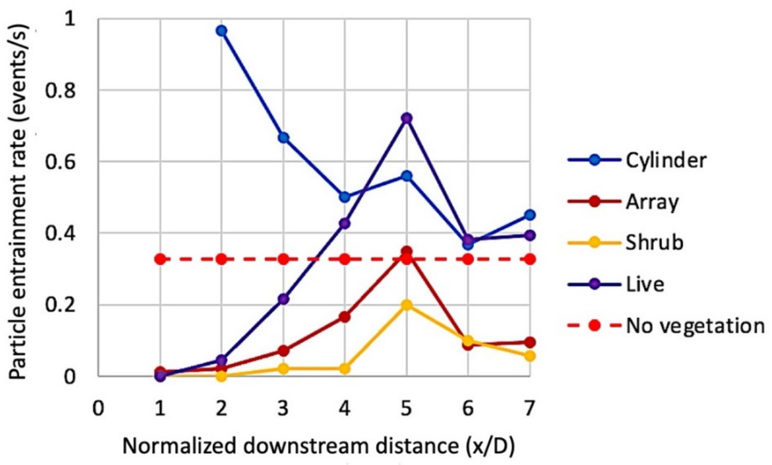
As demonstrated in the previous chapter, the porosity and the vertical distribution of volumetric features of the representative vegetation elements influence the particle entrainment rate by altering the flow properties. From this motivation, the entrainment rate was quantified for the elements of the examined representative vegetation elements at seven consecutive vertical sections (x/D = 1, 2, 3, 4, 5, 6, 7, respectively), as given in Figure 12. A three-minute recording duration was set for particle entrainment tracking by taking advantage of the electric-eye setup (He-Ne laser and the camera). The particle entrainment rate recording duration is deemed to be sufficiently long because for the flow conditions assessed, there were enough repeats to render the recorded mean entrainment rate representative of the experimentally assessed observed rate, which according to the literature can vary from one to a few entrainments per minute [47]. The particle entrainment rate was calculated based on the total number of entrainments read by the optical system and normalized with the total observation duration, (i.e., here three minutes per experimental run). The entrainment occurrences can be manually observed from the video recordings or digitally processed with scientific software via image thresholding and converted into entrainment rate as displayed in Table 2.
As can be seen from Figure 12, the entrainment rate for the cylinder presents a big different trend compared with the other three vegetation elements. It is quite clear that the cylinder has the highest entrainment rate at the x/D = 2 and it decreases gradually along the flow direction. This is in line with the finding by [69,71,73] who state that solid cylinders generate more scouring than the group of cylinders and other vegetation elements. The average entrainment rate of the particle without vegetation is also measured in this case for all seven normalized distances. The particle entrainment rate for the remaining three vegetation elements displays a similar increasing trend until the normalized distance approaches x/D = 5, and then rapidly decreases. This result may reflect the limitations of the He-Ne laser system which cannot completely make a distinction between the motion between full entrainment and twitching. On the other hand, the adjacent fast particle entrainment events are difficult to distinguish by the visual observation method.
To a certain extent, the flow property of turbulence intensity dictates the frequency of particle movement. Comparing the extreme values in Figure 11b and Figure 12, turbulence intensity has the highest value occurring at x/D =1 (for all elements except the shrub), while entrainment rate has the highest value at the normalized distance (x/D) of 5. Turbulence intensity at the nearest distance (, represents turbulence intensity) heavily agrees with the particle entrainment rate (, represents entrainment rate). In other words, just downstream of the obstacle, higher turbulence intensity correlates positively with a higher entrainment rate.
As can be inferred from Figure 12, higher porosity of vegetation elements has a relatively lower entrainment rate except for the specific sample live vegetation, which can be roughly expressed as: . The porosity variation for vegetation elements is listed as: . This result indicates that the shrub vegetation has a certain ability to protect the riverbed destabilization since the lower particle entrainment compared to the entrainment rate measured without vegetation, taking into account spacing between the vegetation within the patch. The porosity of live vegetation shows an unrelated variation to entrainment rate (). This observation is consistent with results reported in [74], concluding that the bending vegetation could decrease the porosity and increase the submerged volume, potentially contributing to higher entrainment rates compared to the array and shrub analogs (Figure 12). Meanwhile, the swaying motion of flexible vegetation is also one of the reasons for increasing the downstream turbulence, promoting velocity fluctuations and rendering them potentially large enough for entraining sediment particles.
Moreover, the values of the entrainment rate displayed in Figure 12 numerically indicate the probability of riverbed destabilization. According to the results, the entrainment rate for the non-porous vegetation element is significantly higher than for other vegetation elements. What comes with this result is that the non-porous vegetation element reflects a higher probability of destabilization. However, this conclusion was not supported here for live vegetation, since the irregular variation of entrainment rate. It is therefore inappropriate to judge the probability of riverbed destabilization only by considering the porosity of vegetation elements under the same flow conditions, without considering the different vegetation categories, which affect turbulence intensity.
The potential particle entrainment events are indicated by the number of impulses exceeding the critical impulse level. The frequency of occurrence for such events indicates the potential particle entrainment rate that is displayed above in Table 3.
The number of impulses calculated in Table 3 were estimated for distinct locations downstream of the vegetation analogs, considering the points from the velocimetry grid (shown with red dots, as illustrated in Figure 6), closest to the upstream face of the exposed test particle (shown with black circles, Figure 6). Figure 13 shows the number of impulses that exceed the critical impulse level () per duration of four-minute measurement downstream of different vegetation elements (defined according to the theory presented in [65]). The following section aims to offer theoretical predictions of the particle entrainment rate through the estimation of the number of flow impulses that are eligible to cause partial or full particle entrainment, at the seven normalized distances downstream each of the four vegetation elements examined herein.
It can be seen clearly from Figure 13 that both elements of array and shrub have the highest number of impulses at the normalized distance equal to five compared to that of other locations. For the case of cylinder, it has the highest number of impulses at the . These results generally agree with the particle entrainment rate measured by the camera and He-Ne laser. For the live vegetation, the highest impulse occurrence rate occurs at the , that is close to the highest particle entrainment rate at the normalized distance at .
The number of the occurrence rate of flow impulses is generally higher to the particle entrainment rate, which is expected given that only a portion of the theoretically estimated impulses are capable of fully entraining the test particle (assuming rolling mode of entrainment [65]), as shown in Figure 14. Compared with the particle entrainment rate, an obvious variation difference for array, shrub, and live vegetation has been observed near the vegetation that they decrease generally with the normalized distance increase until the normalized distance approaching to 3 or 4. The number of impulses variation for cylinder case perfectly matches the trend of particle entrainment rate, with the highest value occurring at the normalized distance , and decreases all the way downstream the vegetation and even has the same local peak at . The comparatively large value near the vegetation element can better explain the practical situation rather than a near-zero value since the sediment entrainment rate determines the riverbed destabilization probability. It can also be clearly seen from the result that each single vegetation element case generally satisfies the variation trend of particle entrainment rate with the normalized distance increasing except for the large value near the element.
A reasonable relationship for the number of impulses at the normalized distance can be distinguished as: . This point is not the best location and way to show the relationship, because they say nothing about the magnitude over which these inequalities span. This result is consistent with the porosity variation of: except for the live vegetation and this difference has been discussed above by [71]. The flexibility of live vegetation corresponds to higher number of impulses and particle entrainment, which is consistent with [71]. It is shown there that flexible vegetation comparatively fostered sediment movement, whereas rigid vegetation prevented riverbed erosion through promoting sediment aggradation.
There exists an interesting trend of increased covariance of the experimentally observed particle entrainment frequency (assessed with the He-Ne laser optical system [75]) and the impulse criterion: at or further downstream of the location x/D = 2, for each vegetation analog, as shown in Figure 14. Another interesting point is that except for the cylinder, the other three vegetation elements have a significant magnitude difference in entrainment rate. Traditionally employed time-averaged flow parameters such as the mean flow velocity and turbulence intensity would be a relatively poor predictor of the probability of particle entrainment and bed surface destabilization for the different types of simulated vegetation assessed herein. However, the impulse criterion presented here is shown to be a more robust and intuitive method to predict the probability of riverbed surface destabilization downstream of the simulated vegetation, as it better correlates with the particle’s entrainment rate (Figure 14). This method can be potentially generalized and applied to a wider range of obstacles to the flow (including both bending and rigid vegetation) to assess riverbed surface destabilization under complex flow environments.
4. Discussion
The obtained results demonstrate that the number of impulse occurrences and camera systems with particles are the potential indicators for riverbed destabilization under different porosity of vegetation elements. To complement the study, our research employed the camera and He-Ne laser system to supplement the findings from the particle entrainment rate and the impulse criterion to account for the entrainment rate downstream emergent and submerge vegetation analogs with different porosity, so as to further link the porosity of instream vegetation to riverbed destabilization.
The porosity variation of vegetation can be expressed as , which is consistent with both of the velocity deficit variation () and the turbulence intensity variation (), at the normalized distance x/D = 1, except for the live, bending vegetation. The observed variation of mean flow velocity and turbulence intensity is consistent with the trends reported in [76] according to which the mean flow velocity is sharply reduced, and the turbulence intensity peaks just downstream various types of instream vegetation. The analysis result based on the different porosity of rigid vegetation could indicate that the variation of the probability of riverbed destabilization is dependent to flow structures such as the flow velocity and the turbulent kinetic energy. Parameters such as the flow velocity and turbulence intensity and derivatives of these have been demonstrated to have a stronger potential in predicting particle entrainment compared to mean shear stresses acting on particles [77]. However, the velocity and the turbulent kinetic energy are still not a robust way for riverbed destabilization estimation since they are flow velocity-based parameters without consideration of other influencing factors such as characteristics of vegetation and riverbed material features defining the resistance to destabilization. In addition, the probability of riverbed destabilization could not be reflected by the porosity when the flexible vegetation was involved since the flow structures of bending vegetation do not vary with the porosity accordingly as the rigid vegetation. Therefore, for different vegetation categories, porosity may need to be used as a variable instead of a constant to assess the riverbed destabilization potential. By using the impulse criterion and the proposed optical system, novel practical ways of assessing riverbed destabilization potential downstream different kinds of vegetation are offered herein. The practicality of the conducted research suggests that the impulse method has the potential to become a suitable criterion that can outperform the traditional methods (such as mean flow velocity, turbulence intensity, TKE, and shear stress) to assess the destabilization of riverbed surface downstream vegetation elements.
The conventional flow structures vary with porosity accordingly and regularly, especially for rigid vegetation under a variety range of flow conditions. When comparing flexible (bending) and solid (no-bending) vegetation, judgment based on porosity may loss its ability to assess the riverbed destabilization. This study overcomes the irregular variation of bending vegetation by shedding more light on the impulse criterion and the camera system with particles. Both the impulse criterion and camera system methods have been experimentally verified to offer better performance compared to other time-averaged flow parameters (such as the depth-averaged mean flow velocity and turbulence intensity, shown in Figure 11) to accurately estimate the particle entrainment rate. The He-Ne laser system may not be very sensitive for detecting all instantaneous particle entrainment events and it may find limited application in the presence of flows carrying suspended sediment blocking visual observations. In such cases, the velocimetry obtained flow impulses offer a better predictor for riverbed destabilization assessment compared to the He-Ne laser system. Another possibility for this result of magnitude difference has been discussed by [15,78,79] that not all the exceedances () of impulse are associated with the particle dislodgement. That means the number of calculated impulses above the critical level is slightly larger than it should be. In summary, there are two reasons for the magnitude difference between particle entrainment occurrence rate calculated by impulse theory and measured by the He-Ne laser system: the overestimation of impulse statistics and the underestimation of the number of particle entrainment with the He-Ne laser system in terms of lower sensitivity for instantaneous movement. This implies that the impulse is much better for predicting the entrainment of particles compared with previous parameters.
On the other hand, Ref. [69] introduced an instrumented particle with a miniaturized size of 3 cm that was also employed by [80] for the riverbed destabilization potential assessment through the embedded sensors to directly record the entrainment event, even for slight movements. An instrumented particle (7 cm in diameter) employed by [81,82] could help investigate sediment particle entrainment and transport in complex environmental flows (such as severe flooding events or high turbidity or flow mixing and transport of sediment). All these aforementioned instrumented particles have been tested downstream of the second group of vegetation (with porosity of 1.25%, 3.25%, 6.25%, 11.25%, and 17.25%) but without any entrainment of instrumented particles being recorded during the 3 min testing period. Consequently, for the riverbed sediment size smaller than 3 cm or a complex flow environment (e.g., flooding), the instrumented particle may not have the ability to record entrainments and assess riverbed destabilization. Finally, this method is of exploratory significance because it enables assessing and characterizing the riverbed destabilization potential for a wider range of river environments including various vegetation types.
5. Conclusions
Riverbed assessments are still far from robust and accurate, and no standard devices or formulas are available to measure them. The dynamic interaction among parameters of vegetation elements, flow properties, and particle entrainment may help engineers design better instream vegetation to sustainably stabilize the riverbed. In this report, the effect of different vegetation, categorized by porosity, on the entrainment rate and the corresponding destabilization probability have been investigated utilizing a 15 mm diameter particle with the help of an ADV, He-Ne laser, and camera. It is shown that using instrumented particles for assessing the risk of riverbed destabilization downstream of vegetation elements is a robust, relatively cost-effective, and practical tool. Furthermore, the impulse criterion is for the first time demonstrated to be a good predictor of the riverbed destabilization risk, assessed experimentally via the particle entrainment rates (observed using an optical setup).
According to the results of this investigation, lower porous vegetation elements caused higher velocity reduction in the flow. Near vegetation elements, turbulence intensity highly agreed with the overall averaged entrainment rate. However, the porosity is a potential parameter for riverbed destabilization only downstream rigid vegetation instead of for live vegetation with bending in flow. The submerged depth, bending extent, vegetation categories, and environmental conditions are all considered the reasons why the highest porosity of live vegetation has the second-highest entrainment rate. It can be concluded that the lower density of instream vegetation results in a lower frequency of particle entrainment, which means a lower probability of riverbed destabilization. From the perspective of geomorphological implications, live vegetation is not suggested as the soft-engineering approach to prevent riverbed destabilization compared with the other rigid vegetation elements under the same porosity condition.
The utility of an optical (He-Ne laser and camera) system in directly assessing the risk of riverbed destabilization downstream instream vegetation has been experimentally demonstrated herein, for the first time. In addition, the presented hydrodynamic analysis also demonstrates that the number of impulses is the best predictor of particle entrainment downstream of the different types of simulated instream vegetation elements. This can be achieved by recording flow turbulence near the riverbed surface to derive the flow impulses carrying enough momentum towards sediment entrainment. Flow impulses embed within them both the influence of mean and turbulent flow fields as well as the duration of flow events above the critical level for particle entrainment downstream vegetation elements. This is the first experimental demonstration of the robust application of the impulse criterion in predicting bed surface destabilization downstream instream vegetation, beyond what would be possible if the mean or turbulent flow fields were to be considered alone.
The above work outlines the potential research direction for the future: the optimal positioning of the impulse method and instrumented particle towards obtaining the maximum amount of information for the potential of riverbed destabilization is going to be explored.
Author Contributions
Conceptualization, M.V. and O.Y.; methodology, M.V., O.Y., Ł.P. and Y.X.; software, Y.X.; validation, M.V., P.M. and Y.X.; formal analysis, Y.X.; investigation, M.V. and Y.X.; resources, M.V. and Y.X.; data curation, M.V. and Y.X.; writing—original draft preparation, Y.X.; writing—review and editing, M.V., G.G., P.M., O.Y., Ł.P. and Y.X.; visualization, Y.X. and M.V.; supervision, M.V.; project administration, M.V.; funding acquisition, M.V. and G.G. All authors have read and agreed to the published version of the manuscript.
Funding
This work has been supported in part by the Royal Society (Research Grant RG2015 R1 68793/1), the Royal Society of Edinburg (Crucible Award), the Carnegie Trust for the Universities of Scotland (project 7066215), the Croatian Science Foundation under the project R3PEAT (UIP-2019-04-4046) and the Polish Ministry of Education and Science.
Institutional Review Board Statement
Not applicable.
Informed Consent Statement
Not applicable.
Data Availability Statement
All data are presented in the main text.
Conflicts of Interest
The authors declare no conflict of interest.
Notation
| The approaching area of particle to the flow. |
| Buoyancy force. |
| Drag coefficient. |
| Added mass coefficient. |
| Diameter of the solid rod. |
| Bridge pier diameter. |
| Frequency of particle entrainment. |
| Hydrodynamic mass coefficient. |
| Drag force. |
| Lift force. |
| Impulse. |
| Critical impulse. |
| Threshold impulse level. |
| Turbulence kinetic energy. |
| Length of lever arm. |
| Vegetation porosity. |
| Entrainment rate of particle. |
| Time. |
| Flow velocity. |
| Critical velocity. |
| Volume of particle. |
| Weight of particle. |
| Distance downstream pier model. |
| Angle between scour slope and riverbed. |
| Density of water. |
| Riverbed material density. |
| Coefficient. |
| Pivoting angle. |
| Impulse exceedance. |
References
- Pandey, M.; Valyrakis, M.; Qi, M.; Sharma, A.; Lodhi, A.S. Experimental assessment and prediction of temporal scour depth around a spur dike. Intl. J. Sed. Res. 2020, 36, 17–28. [Google Scholar] [CrossRef]
- Michalis, P.; Konstantinidis, F.; Valyrakis, M. The road towards Civil Infrastructure 4.0 for proactive asset management of critical infrastructure systems. In Proceedings of the 2nd International Conference on Natural Hazards & Infrastructure (ICONHIC), Chania, Greece, 23–26 June 2019. [Google Scholar]
- Michalis, P.; Vintzileou, E. The Growing Infrastructure Crisis: The Challenge of Scour Risk Assessment and the Development of a New Sensing System. Infrastructures 2022, 7, 68. [Google Scholar] [CrossRef]
- Forzieri, G.; Feyen, L.; Russo, S.; Vousdoukas, M.; Alfieri, L.; Outten, S.; Migliavacca, M.; Bianchi, A.; Rojas, R.; Cid, A. Multi-hazard assessment in Europe under climate change. Clim. Chang. 2016, 137, 105–119. [Google Scholar] [CrossRef]
- Couper, P.R.; Maddock, I.P. Subaerial river bank erosion processes and their interaction with other bank erosion mechanisms on the river arrow, Warwickshire, UK. Earth Surf. Processes Landf. 2001, 26, 631–646. [Google Scholar] [CrossRef]
- Thorne, C.R.; Hey, R.D.; Newson, M.D. Applied Fluvial Geomorphology for River Engineering and Management; John Wiley & Sons: Chichester, UK, 1997. [Google Scholar]
- Solari, L.; Van Oorschot, M.; Belletti, B.; Hendriks, D.; Rinaldi, M.; Vargas-Luna, A. Advances on modelling riparian vegetation—Hydromorphology interactions. River Res. Appl. 2016, 32, 164–178. [Google Scholar] [CrossRef]
- Hardy, R.J. Fluvial geomorphology. Prog. Phys. Geogr. 2006, 30, 553–567. [Google Scholar] [CrossRef]
- Jarvela, J. Flow resistance of flexible and stiff vegetation: A flume study with natural plants. J. Hydrol. 2002, 269, 44–54. [Google Scholar] [CrossRef]
- Wang, P.; Wang, C.; Zhu, D.Z. Hydraulic Resistance of Submerged Vegetation Related to Effective Height. J. Hydrog. 2010, 22, 265–273. [Google Scholar] [CrossRef]
- Nepf, H.M. Hydrodynamics of vegetated channels. J. Hydraul. Res. 2012, 50, 262–279. [Google Scholar] [CrossRef]
- Przyborowski, Ł.; Łoboda, A.M.; Bialik, R.J. Effect of two distinct patches of Myriophyllum species on downstream turbulence in a natural river. Acta Geoph. 2019, 67, 987–997. [Google Scholar] [CrossRef] [Green Version]
- Najafzadeh, M.; Oliveto, G. Riprap incipient motion for overtopping flows with machine learning models. J. Hydroinform. 2020, 22, 749–767. [Google Scholar] [CrossRef]
- Najafzadeh, M.; Rezaie-Balf, M.; Tafarojnoruz, A. Prediction of riprap stone size under overtopping flow using data-driven models. Int. J. River Basin Manag. 2018, 16, 505–512. [Google Scholar] [CrossRef]
- Valyrakis, M.; Diplas, P.; Dancey, C.L. Entrainment of coarse grains in turbulent flows: An extreme value theory approach. Water Resour. Res. 2011, 47, W09,512,3399. [Google Scholar] [CrossRef]
- Carollo, F.G.; Ferro, V.; Termini, D. Flow velocity measurements in vegetated channels. J. Hydraul. Eng. 2002, 128, 664–673. [Google Scholar] [CrossRef]
- Poggi, D.; Porporato, A.; Ridolfi, L.; Albertson, J.; Katul, G. The effect of vegetation density on canopy sub-layer turbulence. Bound.-Layer Meteorol. 2004, 111, 565–587. [Google Scholar] [CrossRef]
- Liu, D.; Diplas, P.; Fairbanks, J.D.; Hodges, C.C. An experimental study of flow through rigid vegetation. J. Geophys. Res. 2008, 113, F04015. [Google Scholar] [CrossRef]
- Hopkinson, L.; Wynn, T. Vegetation impacts on near bank flow. Ecohydrology 2009, 2, 404–418. [Google Scholar] [CrossRef]
- Nepf, H.M. Flow and Transport in Regions with Aquatic Vegetation. Annu. Rev. Fluid Mech. 2012, 44, 123–142. [Google Scholar] [CrossRef]
- Yager, E.; Schmeeckle, M. The influence of vegetation on turbulence and bedload transport. J. Geophys. Res. Earth Surf. 2013, 118, 1585–1601. [Google Scholar] [CrossRef]
- Kitsikoudis, V.; Yagci, O.; Kirca, V.S.O.; Kellecioglu, D. Experimental investigation of channel flow through idealized isolated tree-like vegetation. Environ. Fluid Mech. 2016, 16, 1283–1308. [Google Scholar] [CrossRef]
- Yagci, O.; Strom, K. Reach-scale experiments on deposition process in vegetated channel: Suspended sediment capturing ability and backwater effect of instream plants. J. Hydrol. 2022, 608, 127612. [Google Scholar] [CrossRef]
- Hopkinson, L.; Wynn-Thompson, T. Streambank shear stress estimates using turbulent kinetic energy. J. Hydraul. Res. 2012, 50, 320–323. [Google Scholar] [CrossRef]
- Bouteiller, L.C.; Venditti, J.G. Sediment transport and shear stress partitioning in a vegetated flow. Water Resour. 2015, 51, 2901–2922. [Google Scholar] [CrossRef]
- Shields, A. Anwendung der Ahnlichkeitsmechanik und der Turbulentzforschung die Geshiebebewegung. Ph.D. Thesis, Technical University Berlin, Berlin, Germany, 1936. [Google Scholar]
- Leonard, L.A.; Luther, M.E. Flow hydrodynamics in tidal marsh canopies. Limnol. Oceanogr. 1995, 40, 1474–1484. [Google Scholar] [CrossRef]
- Neumeier, U.; Amos, C.L. The influence of vegetation on turbulence and flow velocities in European salt-marshes. Sedimentology 2006, 53, 259–277. [Google Scholar] [CrossRef]
- Liu, C.; Shan, Y. Analytical model for predicting the longitudinal profiles of velocities in a channel with a model vegetation patch. J. Hydrol. 2019, 576, 561–574. [Google Scholar] [CrossRef]
- Link, O.; González, C.; Maldonado, M.; Escauriaza, C. Coherent structure dynamics and sediment particle motion around a cylindrical pier in developing scour holes. Acta Geophys. 2012, 60, 1689–1719. [Google Scholar] [CrossRef]
- Yang, J.Q.; Chung, H.; Nepf, H.M. The onset of sediment transport in vegetated channels predicted by turbulent kinetic energy. Geophys. Res. Lett. 2016, 43, 11,261-11,268. [Google Scholar] [CrossRef]
- Graf, W.H. Hydraulics of Sediment Transport; McGraw-Hill Book, Co.: New York, NY, USA, 1971. [Google Scholar]
- Garde, R.J.; Ranga Raju, K.G. Mechanics of Sediment Transportation Alluvial Stream Problems; Wiley Eastern Ltd.: New Delhi, India, 1987. [Google Scholar]
- Krey, H. Grenzen der Übertragbarkeit der Versuchsergebnisse und Modellähnlichkeit bei praktischen Flussbauversuchen. Z. Angew. Math. Mech. 1925, 5, 484–486. [Google Scholar]
- Neill, C.R. Mean-velocity criterion for scour of coarse uniform bed-material. In Proceedings of the 12th Congress of the International Association for Hydraulics Research, Fort Collins, CO, USA, 11–14 September 1967; Volume 3, pp. 46–54. [Google Scholar]
- Egiazaroff, I.V. Discussion of “Sediment transportation mechanics: Initiation of motion” by V. A. Vanoni et al. J. Hydraul. Div. Am. Soc. Civ. Eng. 1967, 93, 281–287. [Google Scholar]
- Knoroz, V.S. Non-Eroding Velocity for Fine Sand; Hydrotech Construct: Moscow, Russia, 1953; pp. 21–24. (In Russian) [Google Scholar]
- Bagnold, R.A. An empirical correlation of bedload transport rates in flumes and natural rivers. Math. Phys. Sci. 1980, 372, 453–473. [Google Scholar]
- Bettess, R. Initiation of sediment transport in gravel streams. Proc. Inst. Civ. Eng. 1984, 407, 79–88. [Google Scholar]
- Bathurst, J.C. Critical conditions for bed material movement in steep, boulder-bed streams. Erosion and Sedimentation in the Pacific Rim. In Proceedings of the Symposium, Corvallis, OR, USA, 3–7 August 1987; Beschta, R.L., Blinn, T., Grant, G.E., Ice, G.G., Swanson, F.J., Eds.; IAHS Publ. No. 165; IAHS-AISH Publication: Oxfordshire, UK, 1987; pp. 309–318. [Google Scholar]
- Komar, P.D. Entrainment of sediments from deposits of mixed grain sizes and densities. In Advances in Fluvial Dynamics and Stratigraphy; Carling, P.A., Dawson, M.R., Eds.; John Wiley and Sons Ltd.: Hoboken, NJ, USA, 1996; pp. 127–181. [Google Scholar]
- Nelson, J.M.; Shreve, R.L.; McLean, S.R.; Drake, T.G. Role of near-bed turbulence structure in bed load transport and bed form mechanics. Water Resour. Res. 1995, 31, 2071–2086. [Google Scholar] [CrossRef]
- Sumer, B.M.; Chua, L.H.; Cheng, N.-S.; Fredsøe, J. Influence of turbulence on bedload sediment transport. J. Hydraul. Eng. 2003, 129, 585–596. [Google Scholar] [CrossRef]
- Nino, Y.; Garcia, M. Experiments on particle–turbulence interactions in the near-wall region of an open channel flow: Implications for sediment transport. J. Fluid Mech. 1996, 326, 285–319. [Google Scholar] [CrossRef]
- Smart, G.; Habersack, H. Pressure fluctuations and gravel entrainment in rivers. J. Hydraul. Res. 2007, 45, 661–673. [Google Scholar] [CrossRef]
- Feng, Z.; Tan, G.; Xia, J.; Shu, C.; Chen, P.; Yi, R. Two- dimensional numerical simulation of sediment transport using improved critical shear stress methods. Int. J. Sediment Res. 2019, 35, 15–26. [Google Scholar] [CrossRef]
- Diplas, P.; Dancey, C.L.; Celik, A.O.; Valyrakis, M.; Greer, K.; Akar, T. The role of impulse on the initiation of particle movement under turbulent flow conditions. Science 2008, 322, 717–720. [Google Scholar] [CrossRef]
- Tinoco, R.O.; Coco, G. A laboratory study on sediment resuspension within arrays of rigid cylinders. Adv. Water Resour. 2016, 92, 1–9. [Google Scholar] [CrossRef]
- Tinoco, R.; Coco, G. Turbulence as the main driver of resuspension in oscillatory flow through vegetation. J. Geophys. Res. Earth Surf. 2018, 123, 891–904. [Google Scholar] [CrossRef]
- Schmeeckle, M.W.; Nelson, J.M.; Shreve, R.L. Forces on stationary particles in near-bed turbulent flows. J. Geophys. Res. 2007, 112, F02003. [Google Scholar] [CrossRef]
- Gimenez-Curto, L.A.; Corniero, M.A. Entrainment threshold of cohesionless sediment grains under steady flow of air and water. Sedimentology 2009, 56, 493–509. [Google Scholar] [CrossRef]
- Hubble, T.C.T.; Docker, B.B.; Rutherfurd, I.D. The role of riparian trees in maintaining riverbank stability: A review of Australian experience and practice. Ecol. Eng. 2010, 36, 291–304. [Google Scholar] [CrossRef]
- Perona, P.; Molnar, P.; Savina, M.; Burlando, P. An observation-based stochastic model for sediment and vegetation dynamics in the floodplain of an alpine braided river. Water Resour. Res. 2009, 45, W09418. [Google Scholar] [CrossRef]
- Millar, R.G.; Quick, M.C. Effects of bank stability on geometry of gravel rivers. J. Hydraul. Eng. 1993, 119, 1343–1363. [Google Scholar] [CrossRef]
- Czarnomski, N.M.; Tullos, D.D.; Thomas, R.E.; Simon, A. Effects of Vegetation Canopy Density and Bank Angle on Near-Bank Patterns of Turbulence and Reynolds Stresses. J. Hydraul. Eng. 2012, 138, 974–978. [Google Scholar] [CrossRef]
- Wilson, C.A.M.E.; Stoesser, T.; Bates, P.D.; Pinzon, A.B. Open channel flow through different forms of submerged flexible vegetation. J. Hydraul. Eng. 2003, 129, 847–853. [Google Scholar] [CrossRef]
- Sand-Jensen, K. Influence of submerged macrophytes on sediment composition and near-bed flow in lowland streams. Freshw. Biol. 1998, 39, 663–679. [Google Scholar] [CrossRef]
- Wang, C.; Zheng, S.; Wang, P.F.; Hou, J. Interactions between vegetation, water flow and sediment transport: A review. J. Hydrog. 2015, 27, 24–37. [Google Scholar] [CrossRef]
- Jalonen, J.; Järvelä, J. Estimation of drag forces caused by natural woody vegetation of different scales. J. Hydrodyn. Ser. B 2014, 26, 608–623. [Google Scholar] [CrossRef]
- Liu, D.; Diplas, P.; Hodges, C.C.; Fairbanks, J.D. Hydrodynamics of flow through double-layer rigid vegetation. Geomorphology 2010, 116, 286–296. [Google Scholar] [CrossRef]
- Nepf, H.M. Drag, turbulence, and diffusion in flow through emergent vegetation. Water Resour. Res. 1999, 35, 479–489. [Google Scholar] [CrossRef]
- Yagci, O.; Yildirim, I.; Celik, M.F.; Kitsikoudis, V.; Duran, Z.; Kirca, V.S.O. Clear water scour around a finite array of cylinders. Appl. Ocean. Res. 2017, 68, 114–129. [Google Scholar] [CrossRef]
- Liu, C.; Hu, Z.; Lei, J.; Nepf, H. Vortex structure and sediment deposition in the wake behind a finite patch of model submerged vegetation. J. Hydraul. Eng. ASCE 2018, 144, 04017065. [Google Scholar] [CrossRef]
- Liu, C.; Nepf, H. Sediment deposition within and around a finite patch of model vegetation over a range of channel velocity. Water Resour. Res. 2016, 52, 600–612. [Google Scholar] [CrossRef]
- Valyrakis, M.; Diplas, P.; Dancey, C.L.; Greer, K.; Celik, A.O. The role of instantaneous force magnitude and duration on particle entrainment. J. Geophys. Res. 2010, 115, 1–18. [Google Scholar] [CrossRef]
- Yagci, O.; Celik, M.F.; Kitsikoudis, V.; Ozgur Kirca, V.S.; Hodoglu, C.; Valyrakis, M.; Duran, Z.; Kaya, S. Scour patterns around isolated vegetation elements. Adv. Water Resour. 2016, 97, 251–265. [Google Scholar] [CrossRef]
- Valyrakis, M.; Liu, D.; Turker, U.; Yagci, O. The role of increasing riverbank vegetation density on flow dynamics across an asymmetrical channel. Environ. Fluid Mech. 2021, 21, 643–666. [Google Scholar] [CrossRef]
- SonTek. ADV Field Technical Manual; SonTek/YSI, Inc.: San Diego, CA, USA, 2001. [Google Scholar]
- Al-Obaidi, K.; Xu, Y.; Valyrakis, M. The Design and Calibration of Instrumented Particles for Assessing Water Infrastructure Hazards. J. Sens. Actuator Netw. 9 2020, 3, 36. [Google Scholar] [CrossRef]
- Liu, D.; AlObaidi, K.; Valyrakis, M. The assessment of an Acoustic Doppler Velocimetry profiler from a user’s perspective. Acta Geophys. 2022, 434, 87–89. [Google Scholar] [CrossRef]
- Yagci, O.; Tschiesche, U.; Kabdasli, M.S. The role of different forms of natural riparian vegetation on turbulence and kinetic energy characteristics. Adv. Water Resour. 2010, 33, 601–614. [Google Scholar] [CrossRef]
- Yagci, O.; Karabay, O.; Strom, K. Bleed flow structure in the wake region of finite array of cylinders acting as an alternative supporting structure for foundation. J. Ocean. Eng. Mar. Energy 2021, 7, 379–403. [Google Scholar] [CrossRef]
- Yagci, O.; Kitsikoudis, V.; Celik, M.F.; Hodoglu, C.; Kirca, V.S.O.; Valyrakis, M.; Duran, Z.; Kaya, S. The variation of local scour pattern around representative natural vegetation elements. In Proceedings of the 2016, 36th IAHR Congress, The Hague, The Netherlands, 28 June–3 July 2015. [Google Scholar]
- Diehl, R.M.; Merritt, D.M.; Wilcox, A.C.; Scott, M.L. Applying functional traits to ecogeomorphic processes in riparian ecosystems. BioScience 2017, 67, 729–743. [Google Scholar] [CrossRef]
- Diplas, P.; Celik, A.O.; Dancey, C.L.; Valyrakis, M. Nonintrusive method for detecting particle movement characteristics near-threshold flow conditions. J. Irrig. Drain. Eng. ASCE 2010, 136, 774–780. [Google Scholar] [CrossRef]
- Amina; Tanaka, N. Numerical Investigation of 3D Flow Properties around Finite Emergent Vegetation by Using the Two-Phase Volume of Fluid (VOF) Modeling Technique. Fluids 2022, 7, 175. [Google Scholar] [CrossRef]
- Yager, E.M.; Venditti, J.G.; Smith, H.J.; Schmeeckle, M.W. The trouble with shear stress. Geomorphology 2018, 323, 41–50. [Google Scholar] [CrossRef]
- Celik, A.O.; Diplas, P.; Dancey, C.L.; Valyrakis, M. Impulse and Particle Dislodgement under Turbulent Flow Conditions. Phys. Fluids 2010, 22, 1–13. [Google Scholar] [CrossRef]
- Xu, Y.; Valyrakis, M. Monitoring the potential for bridge protections destabilization, using instrumented particles. In Proceedings of the International Conference on Fluvial Hydraulics River Flow, Delft, The Netherlands, 7–10 July 2020; p. 0144. [Google Scholar]
- Al-Obaidi, K.; Valyrakis, M. Linking the explicit probability of entrainment of instrumented particles to flow hydrodynamics. Earth Surf. Processes Landf. 2021, 46, 2448–2465. [Google Scholar] [CrossRef]
- AlHusban, Z.; Valyrakis, M. Assessing sediment transport dynamics from energy perspective by using the smart sphere. Intl. J. Sed. Res. 2022, in press. [Google Scholar] [CrossRef]
- Alhusban, Z.; Valyrakis, M. Assessing and Modelling the Interactions of Instrumented Particles with Bed Surface at Low Transport Conditions. Appl. Sci. 2021, 11, 7306. [Google Scholar] [CrossRef]
Figure 1.
Sketch of the physical processes leading to the destabilization of the riverbed surface downstream of the instream vegetation, in an open channel flow (with mean flow velocity U and depth Y); the exposed particle (black closed circle) resting on the riverbed surface, is swept away (dashed open circle) by a coherent flow structure.

Figure 2.
Schematic diagram of the side and top views of the experimental flume. Vertical green dashed lines denote the corresponding components between the two views.
Figure 2.
Schematic diagram of the side and top views of the experimental flume. Vertical green dashed lines denote the corresponding components between the two views.

Figure 3.
The first experimental group of vegetation analogs with a diagrammatic sketch and picture; the circle under each sketch represents the maximum diameter of the corresponding vegetation element.
Figure 3.
The first experimental group of vegetation analogs with a diagrammatic sketch and picture; the circle under each sketch represents the maximum diameter of the corresponding vegetation element.

Figure 4.
Demonstration of the simulated vegetation elements comprising the second experimental group design for different porosity () of vegetation; smaller circles (of diameter d) represent the rod diameter used to simulate the individual element within the vegetation patch, identified with Ci (where i the number of rods within the patch).

Figure 5.
(a) Perspective view of the test section involving the 3D printed layer of spherical uniformly sized particles (with diameter 2.5 cm) downstream of the flow obstacle. Particle entrainments are validated with the top view camera (see holder above the water surface) and flow measurements are obtained with the Vectrino I® ADV (Nortek, 1351 Rud, Norway); (b) top view of the 3D printed bed surface along with the different patch densities; and (c) side view of the different patch densities used.

Figure 6.
Sketch of the experimental test section showing the flow measurement grid comprising of point locations of ADV velocity measurements (red points) downstream the vegetation element (represented with a black rectangle on the upstream), and the bed surface locations for placing the instrumented particle (black circles).

Figure 7.
Photos of various developed instrumented particle designs with different external diameters of: (a) 70 mm, (b) 40 mm, (c) 30 mm, and (d) 20 mm; and (e) a spherical particle with 15 mm diameter, resting on a 3D printed bed of unisize bed material, also showing the pin restricting the full downstream entrainment of the spherical particle.


Figure 8.
Photographs taken from the camera demonstrate the two main stage characteristics of the particle entrainment process; (a) the exposed particle in the fully displaced position (the pin restraining its downstream motion), partially covering the He-Ne laser beam which is detected by the camera; (b) the exposed particle remains in its resting pocket and the He-Ne laser beam is not partially targeting the particle (state of no entrainment).

Figure 9.
Side-view of the flume with the He-Ne laser and camera partially targeting the exposed particle downstream of the live vegetation element.
Figure 9.
Side-view of the flume with the He-Ne laser and camera partially targeting the exposed particle downstream of the live vegetation element.

Figure 10.
Stream-wise velocity profiles for the characteristic types of vegetation elements used in the experiments.
Figure 10.
Stream-wise velocity profiles for the characteristic types of vegetation elements used in the experiments.

Figure 11.
Variation of (a) depth-averaged mean flow velocity, and (b) turbulence intensity under different vegetation analogs.
Figure 11.
Variation of (a) depth-averaged mean flow velocity, and (b) turbulence intensity under different vegetation analogs.

Figure 12.
Entrainment rate variation downstream the vegetation elements measured by the He-Ne laser system with the averaged entrainment rate without vegetation.
Figure 12.
Entrainment rate variation downstream the vegetation elements measured by the He-Ne laser system with the averaged entrainment rate without vegetation.

Figure 13.
The variation of frequency is calculated by the number of impulses () above a critical level over a four-minute period at different normalized distance (x/D) for the four vegetations elements.
Figure 13.
The variation of frequency is calculated by the number of impulses () above a critical level over a four-minute period at different normalized distance (x/D) for the four vegetations elements.

Figure 14.
Comparison of entrainment rates estimated using the theoretical impulse method and experimental observations (using the He-Ne laser system) for the characteristic types of vegetation elements used in the experiments.
Figure 14.
Comparison of entrainment rates estimated using the theoretical impulse method and experimental observations (using the He-Ne laser system) for the characteristic types of vegetation elements used in the experiments.


Table 1.
Instream vegetation characteristics with different number of rigid dowels and density.
| N | 5 | 13 | 25 | 45 | 69 | NA |
| (%) | 1.25 | 3.25 | 6.25 | 11.25 | 17.25 | 100 |
Table 2.
Entrainment rate along the normalized distance for different vegetation elements.
| Elements | x/D = 1 | x/D = 2 | x/D = 3 | x/D = 4 | x/D = 5 | x/D = 6 | x/D = 7 | |
|---|---|---|---|---|---|---|---|---|
| Emergent | Cylinder | - | 0.976 | 0.667 | 0.500 | 0.561 | 0.367 | 0.450 |
| Array | 0.011 | 0.022 | 0.072 | 0.167 | 0.350 | 0.089 | 0.094 | |
| Shrub | 0.000 | 0.000 | 0.022 | 0.022 | 0.200 | 0.100 | 0.056 | |
| Submerge | Live | 0.000 | 0.044 | 0.217 | 0.428 | 0.722 | 0.383 | 0.394 |
| No vegetation | 0.328 | 0.328 | 0.328 | 0.328 | 0.328 | 0.328 | 0.328 | |
Table 3.
The number of impulses that exceeds critical level during one-second duration () at the seven measurement positions for different vegetation elements.
Table 3.
The number of impulses that exceeds critical level during one-second duration () at the seven measurement positions for different vegetation elements.
| Elements | x/D = 1 | x/D = 2 | x/D = 3 | x/D = 4 | x/D = 5 | x/D = 6 | x/D = 7 | |
|---|---|---|---|---|---|---|---|---|
| Emergent | Cylinder | 0.514 | 1.282 | 1.091 | 0.544 | 0.719 | 0.366 | 0.070 |
| Array | 1.693 | 1.537 | 0.627 | 1.055 | 2.73 | 0.394 | 0.882 | |
| Shrub | 0.542 | 0.044 | 0.182 | 0.464 | 0.931 | 0.732 | 0.704 | |
| Submerge | Live | 2.414 | 1.806 | 1.106 | 0.076 | 1.234 | 3.7 | 1.613 |
Publisher’s Note: MDPI stays neutral with regard to jurisdictional claims in published maps and institutional affiliations. |
© 2022 by the authors. Licensee MDPI, Basel, Switzerland. This article is an open access article distributed under the terms and conditions of the Creative Commons Attribution (CC BY) license (https://creativecommons.org/licenses/by/4.0/).
Share and Cite
MDPI and ACS Style
Xu, Y.; Valyrakis, M.; Gilja, G.; Michalis, P.; Yagci, O.; Przyborowski, Ł. Assessing Riverbed Surface Destabilization Risk Downstream Isolated Vegetation Elements. Water 2022, 14, 2880. https://doi.org/10.3390/w14182880
AMA Style
Xu Y, Valyrakis M, Gilja G, Michalis P, Yagci O, Przyborowski Ł. Assessing Riverbed Surface Destabilization Risk Downstream Isolated Vegetation Elements. Water. 2022; 14(18):2880. https://doi.org/10.3390/w14182880
Chicago/Turabian StyleXu, Yi, Manousos Valyrakis, Gordon Gilja, Panagiotis Michalis, Oral Yagci, and Łukasz Przyborowski. 2022. "Assessing Riverbed Surface Destabilization Risk Downstream Isolated Vegetation Elements" Water 14, no. 18: 2880. https://doi.org/10.3390/w14182880
Note that from the first issue of 2016, this journal uses article numbers instead of page numbers. See further details here.