Article

A Comparative Study on 2D CFD Simulation of Flow Structure in an Open Channel with an Emerged Vegetation Patch Based on Different RANS Turbulence Models

1
State Key Laboratory of Water Resources and Hydropower Engineering Science, Wuhan University, Wuhan 430072, China
2
Science and Technology Research Institute, China Three Gorges Corporation, Beijing 100038, China
3
State Key Laboratory of Hydrology-Water Resources and Hydraulic Engineering, Hohai University, Nanjing 210098, China
*
Author to whom correspondence should be addressed.
Water 2022, 14(18), 2873; https://doi.org/10.3390/w14182873
Submission received: 17 August 2022 / Revised: 10 September 2022 / Accepted: 12 September 2022 / Published: 15 September 2022
(This article belongs to the Special Issue Fluvial Hydraulics in the Presence of Vegetation in Channels)

Abstract

:
Aquatic plants widely exist in rivers, which can affect the flow structure in rivers and have an important impact on the evolution of river morphology. The emerged vegetation is an important member of aquatic vegetation in the river, so studying the flow structure around the emerged vegetation patches is of great significance. Computational fluid dynamics (CFD) simulation provides support for the related research works. Applying the appropriate turbulence model is crucial to achieving realistic numerical simulation results. In this study, two-dimensional numerical simulations were carried out and compared with experimental data by six different Reynolds-Averaged Navier–Stokes (RANS) turbulence models, i.e., Standard k-ε model, Renormalization group (RNG) k-ε model, Realizable k-ε model, Standard k-ω model, Shear-stress transport (SST) k-ω Model, and the Reynolds stress model (RSM). CFD is an effective research method, and the results showed that there are different simulation performances with different turbulence models. The shear stress transport k-ω model achieves the most consistent numerical simulation results with the experimental data for the longitudinal mean flow velocity distribution at the centerline, and the Reynolds stress model provides the least consistent numerical simulation with the experimental data. Then the performance of the six models in simulating the flow field characteristics and longitudinal outflow after vegetation patch was compared.

1. Introduction

Aquatic plants are an important part of the ecological environment and are widely distributed in rivers, lakes, and offshore areas. In natural rivers, aquatic vegetation is generally classified as emerged and submerged, rigid and flexible. Positive and negative feedback widely exists between various aquatic vegetation and river morphology [1]. Vegetation can affect sediment transport and flow structure. The density and arrangement of vegetation affect the water flow to some extent, and the increase in plant density also increases flow resistance [2]. The significance of the interaction between aquatic plants and water flow in natural rivers must be studied. Zong and Nepf represented vegetation patches and plants with 2D circular porous obstruction and rigid cylinders, respectively, because rigid cylinders can approximately simulate stems [3]. They also experimentally investigated the turbulent wake behind a single 2D emerged vegetation patch, described the length and stability of this wake and investigated the effect of patch diameter and porosity on this wake [3]. This type of simulation has also been used in many studies. Liu et al. studied the resistance estimation of rigid submerged vegetation using similar cylindrical arrays [4]. Caroppl et al. measured the characteristics of wake flows after a real riparian vegetation patch and found that the presence of leaves is a key factor in the obstructing effect of vegetation patches on water flow [5]. Huai and Zhang et al. conducted physical experiments to study the flow structure near flexible submerged aquatic vegetation with leaves [6]. By contrast, cylindrical arrays are easy to implement and are effective in simulating vegetation patches. Yu and Shan et al. conducted experiments using rigid cylinders as representative of vegetation to investigate the wake structure behind an individual vegetation patch and found that variations in the density and length of vegetation patches along the streamwise direction affect the steady wake flow [7]. White and Nepf also used rigid cylindrical arrays to represent aquatic plants and performed laboratory experiments to study and characterize the flow structure and characteristics around the cylindrical arrays [8]. Related numerical simulation studies also simulated vegetation communities as rigid cylinder arrays. Liu and Huai et al. studied the flow structure and characteristics around submerged vegetation patches through three-dimensional CFD numerical simulation [9]. Because of the important influence of aquatic vegetation on rivers, further research is necessary to study the interaction between aquatic plant patches and water flow, which is also the starting point of the current work.
Computational fluid dynamics (CFD), a branch of fluid dynamics, is an available and reliable tool commonly used in various research fields. CFD provides an operational platform for engineers to simulate actual working conditions and has been widely used to study the interaction between water flow and aquatic plants. RANS, large eddy simulation (LES), and direct numerical simulation are currently the main methods for numerical fluid simulation. Common turbulent flow models include the Spalart–Allmaras model, standard k-ε model, RNG k-ε model, realizable k-ε model, standard k-ω model, SST k-ω model, Reynolds stress model (RSM), and LES, etc. An important research step is to choose a proper turbulence model to describe the turbulence. Liu and Huai et al. conducted a numerical simulation on the resistance characteristics of rigid submerged vegetation, in which LES was used to simulate the flow around the vegetation patches [10]. Liu and Chen used an improved RNG k-ε turbulence model to simulate the flow in open waters and vegetation waters. The predicted results are in good agreement with the experimental data, proving that the improved RNG k-ε turbulence model has good performance in the flow field near vegetation [11]. Liu and Huai et al. used 3D LES to numerically study hydrodynamics in open channels with an array of square vegetation patches that are discontinuously distributed along the river bank. They found that LES performs well in predicting the variation of turbulence structure with different densities and distances of vegetation array [12]. Anjum and Ghani et al. developed a 3D geometric model to study the internal flow structure of a two-layer vegetated patch, which was solved with the 3D RSM to obtain the distribution of mean velocity and Reynolds stress at different flow rates [13]. Anjum and Tanaka used RSM for 3D numerical simulations to investigate the turbulent flow characteristics of water flow in a channel arranged with double-layered vegetation, submerged vegetation, and emerged vegetation with the same vegetation density [14]. Meanwhile, different works have used different turbulent flow models for the simulation of turbulent flow behind vegetation patches in the flow channel. In the case of complex numerical fluid dynamics, the accuracy and efficiency of simulation vary among different turbulent flow models. A comparison of basic turbulence models is currently needed to provide guidance for future research and support the application of CFD in the study of vegetation–water flow interaction.
Submerged vegetation and emerged vegetation are common types of aquatic vegetation in river channels. 2D models are suitable for the numerical simulation of rigid emerged vegetation. Meanwhile, 3D models are usually adopted for the numerical simulation of submerged vegetation patches. For emerged vegetation in rivers, its interaction with water flow has been investigated for vegetation patches of different shapes and distributions. Qu and Yu conducted a 2D numerical simulation of an isolated emerged vegetation patch in a channel. By using a simple formula of flow velocity distribution, this highly simplified method captures the key features of stable wake, wake recovery, and von–Kármán vortex street [15]. Zhan and Hu et al. introduced a nonconstant inertial resistance coefficient and used a porous media approach to numerically simulate the emerged vegetation in a 2D channel. They found that the improved porous media model can reasonably predict water flow [16]. Yamasaki and Lima et al. investigated the interaction between the emerged vegetation patches and water flow by 2D CFD and simulated the evolutionary processes of the patch erosion and growth of emerged vegetation in the channel [17]. Zhu and Yang et al. investigated the evolution trends of vegetation patches using a 2D shallow water equation and simulated the evolutionary behavior of vegetation patches in the river channel by setting different initial conditions [18]. Relevant physical experiments were also conducted. Li and Huai et al. performed laboratory experiments to investigate the hydrodynamics and turbulent structure in a channel with multiple emerged vegetation patches distributed on one side by simplifying the vegetation to rigid groups of fine cylinders and setting different vegetation densities, diameters of vegetation patches, and distances between adjacent vegetation patches [19].
The Reynolds average models have a wide range of applications and require relatively fewer computational costs. The application of RANS-based turbulent flow models in the simulation of turbulence in river channels was investigated. Farhadi and Mayrhofer et al. selected the standard k-ε model and two k-ω models to simulate turbulent structures in a river section of a runway channel. The comparison with the experimental data revealed that all three models underestimated the intensity of turbulence in the river channel, although they were able to achieve good predictions of the mean velocity [20]. Shaheed et al. investigated the comparative simulation performance of the standard k-ε model and realizable k-ε model for flow characteristics in the bends and confluences of an open channel [21]. Only a few comparative studies have been conducted on the performance of RANS-based turbulence models in the numerical simulation of wake after rigid emerged vegetation patches. For the numerical simulation of the interaction between the emerged aquatic vegetation and water flow in an open channel, the applied RANS model varied in different reports. Using the k-ε model, Lina and Nepf conducted a 2D simulation study of the flow field near two adjacent circular vegetation patches of equal diameter and investigated different distributions of two adjacent vegetation patches on the wake and interaction [22]. Brito and Fernandes et al. used the porous media model to carry out the 3D RANS numerical simulation of water flow with submerged vegetated floodplains and obtained the correct simulation [23]. In the current work, a simple numerical simulation experiment of a straight channel arranged with an isolated emerged vegetation patch was performed to investigate the applicability of several existing available turbulent flow models in the simulation of the interaction between the emerged vegetation and water flow. The results of numerical simulations were analyzed and compared with those published by Zong and Nepf [3]. The implementation of the numerical simulation is described in the next section.

2. Materials and Methods

2.1. Numerical Models

The Reynolds–Average model decomposes the instantaneous variables in the Navier–Stokes equations into two parts, the average and the fluctuating. Considering the incompressible turbulent flow without temperature change, the governing equations based on RANS are [24,25,26]:
u ¯ i x i = 0
ρ u ¯ i t + x j ρ u ¯ i u ¯ j + ρ u i u j ¯ = f ¯ i p ¯ x i + τ ¯ i j x j
where u   ¯ and u represent the mean value and fluctuating value of velocity, respectively; ρ represents the density; p ¯ represents the mean pressure; and τ ¯ i j represents the mean viscous stress tensor:
τ ¯ i j = μ u ¯ i x j + u ¯ j x i
The models selected in this paper include the standard k-ε model, RNG k-ε model, realizable k-ε model, standard k-ω model, shear-stress transport (SST) k-ω model, and Reynolds stress model (RSM).

2.1.1. Standard k-ε Model

The standard k-ε model is the most classical two-equation model proposed by Launder and Spalding, which is based on transport equations for the turbulence kinetic energy (k) and the turbulence dissipation rate (ε) [27]. The model is a widely used semi-empirical model, which assumes that the flow is completely turbulent, ignoring the molecular viscosity [28]. For some unconstrained flow, strong swirl, etc., the k-ε model performs poorly [28].

2.1.2. RNG k-ε Model

The RNG k-ε model is a turbulent model derived from the renormalization group theory by Yakhot and Orszag of Princeton University [29]. The RNG k-ε model has a similar form to the standard k-ε model. It improves the standard k-ε model by adding additional source terms to the turbulent kinetic energy dissipation ε transport equation and modifies the large-scale motion and viscosity to remove the influence of small-scale motion [30]. The RNG k-ε model is more suitable for the numerical simulation of flow in a rotating cavity because of its higher accuracy [31].

2.1.3. Realizable k-ε Model

Compared with the standard k-ε model, the realizable k-ε model replaces the original dissipation rate equation and adopts a new realizable eddy viscosity formula. In some comparative test cases, the stability and prediction accuracy of the realizable k-ε model are better than those of the standard k-ε model [32,33]. The realizable k-ε model is more accurate than the standard k-ε model in predicting the dissipation rate of flat and round jets and better in predicting the characteristics of the boundary layer with a large pressure gradient [31].

2.1.4. Standard k-ω Model

The standard k-ω model is based on the Boussinesq assumption and Reynolds average rule. Launder and Spalding (1972) improved and optimized the Kolmogorov model. Wilcox (2006) improved the previous version of the k-ω model and made the eddy viscosity a function of k and ω, thus allowing the model to be applied in extensive situations [34,35,36]. Although the standard k-ω model can well describe the near-wall flow, the boundary conditions and the initial turbulence level can affect the simulation results of some flows very sensitively [31].

2.1.5. SST k-ω Model

The SST k-ω model combines the accurate Wilcox k-ω model in the near wall region and the stable k-ε model in the far field region by introducing functions; in 1993, Menter proposed redefining the eddy viscosity in this model to solve the problem of excessive prediction of eddy viscosity [37]. The good accuracy of the shear pressure transport k-ω model is mainly attributed to its efficient near-wall formulation [38].

2.1.6. RSM

The RSM directly solves the transport equation of each component of the Reynolds stress tensor without applying the isotropic eddy viscosity assumption in the Boussinesq hypothesis [39,40]. Five additional transport equations must be solved in the 2D flow problem. RSM can accurately predict complex flow, making it a precise turbulence model; however, the calculation cost is high, and RSM cannot always obtain more accurate results compared with some simple models [41]. It should be noted that the RSM model used here is based on the ε equation. In some numerical simulation cases of swirl flow, RSM produces the worst results [42].

2.2. Simulation Setup

The arrangement of the numerical simulation in this study was adopted from the work of Zong and Nepf [3]. In the experiments, rigid cylinders were used to represent the aquatic vegetation. The water depth in the channel was smaller than the length of the cylinders, allowing the study of the interaction between an emerged vegetation patch and water flow. Hence, 2D numerical simulation is applicable in this case. In the experiments, the total length of the experimental section was 13 m, the width was 1.2 m, and the channel was kept horizontal. In the numerical simulation, the total length of the calculation domain was 7.01 m (≈31.86 D), and the width was 1.2 m (≈5.45 D), where D represents the diameter of the vegetation patch. Since the measurements in the experiments of Zong and Nepf [3]. were conducted only for part of the experimental segment, the computational domain length of the numerical simulations was shorter than that of the experimental segment to save computational resources. This did not affect the subsequent comparison and analysis. In the experiments, an emerged vegetation patch was simulated by a rigid cylinder group with a diameter of d = 0.6 cm. In the numerical simulation, the vegetation patch was simulated by a hollow circular hole group with a diameter of d = 0.6 cm. The diameter of the rigid emerged vegetation patch was D = 22 cm in the experiments and numerical simulation. In the experiments, the vegetation patches were located in the center of the channel, and the center of the vegetation patches coincided with the centerline of the channel. The waterward front edge was 3 m away from the water inlet. In the numerical simulation, given that the total length of the calculation domain was smaller than the total length of the channel test section in the laboratory, the upstream of the vegetation patch was set as 1.54 m (=7 D) away from the inlet at the center line. The center of the upstream edge of the vegetation patch was the origin of the x-axis, and the x-axis pointed to the flow direction, while the origin of the y-axis was the same as that of the x-axis. Φ represents the average solid volume fraction, a represents the frontal area in unit volume, and n represents the number of cylinders in the unit area. Their relationships were Φ = π a d / 4 and a = n d . In the experiment, the vegetation density of the vegetation patch was   Φ = 0.1 , and the upstream inflow velocity was U = 9.8 ± 0.1 cm/s. In the numerical simulation, the inflow velocity was defined as U = 9.8 cm/s. Reynolds number based on vegetation stem scale d was defined as [2]:
R e d = U d ν
where ν represents the kinematic viscosity coefficient of the water. Figure 1 shows the schematic of the numerical simulation model.
For numerical simulation using the six turbulence models, the same set of grids was shared. The grid was hybrid, and the grid of vegetation patch area and wake area was refined. The total number of grid units was 349 k, where k represents a thousand. Figure 2 shows partial details of the grid.
SIMPLEC was used for pressure–velocity coupling. The steps of the SIMPLEC algorithm are the same as those of SIMPLE, and the correction makes SIMPLEC more economical than SIMPLER and SIMPLE [43]. The same settings were used for the boundary conditions of all numerical simulation cases. The three main types of boundary conditions are inlet, outlet, and wall. The inlet boundary adopted the velocity inlet condition, and the flow velocity was set to 9.8 cm/s. The outlet boundary adopted the pressure outlet condition, and the pressure was set to 0. The wall boundary adopted the non-slip boundary condition, including the boundary on both sides of the calculation domain and the circular holes in the vegetation area. For the non-slip wall boundary in all the cases, the enhanced wall treatment was adopted. The information of all cases is listed in Table 1.

2.3. Model Validation

Transient numerical simulations were used for all of the current cases. Therefore, determining the independence between the number of grid units used in the simulation and the experimental results and proving the independence between the time step and simulation results are necessary. With reasonable grid and time step independence verification, a small number of computational grid cells and a relatively large time step can be selected to obtain the correct results, which will make the computation faster and save computational resources. Table 2 shows the information on the numerical simulation cases used for model validation.

2.3.1. Grid Independence Validation

Numerical cases V, VII, and VIII were selected to verify the mesh independence. The number of grid cells in case VII was 258 k. The grids of cases V and VIII are globally encrypted by the case VII grid. The number of grid cells of case V was 349 k, which is 1.35 times that in case VII. The number of grid cells in case VIII was 489 k, which is 1.40 times that in case V. The longitudinal instantaneous velocity u ¯ at the wake centerline of the simulation results of cases V and VIII was verified to be consistently distributed. Meanwhile, the simulation results of cases VII and VIII showed poor consistency in some regions. This finding proves that the number of grid cells has a great influence on the simulation, but the simulation results are extremely close when the number of grid cells exceeds 349 k. When the number of grid cells in case V continued to increase to a certain extent, the simulation results stabilized, and the grid independence of the case V grid was consequently verified. Only the case V grid was applied in the next section to save computing resources. Figure 3 depicts the longitudinal mean velocity u ¯ at the centerline of cases V, VII, and VIII. Table 3 shows several numerical simulation data of three cases for grid independence validation. The longitudinal flow velocity u and the transverse coordinate x are dimensionless and expressed as u ¯ / U and x / D , respectively.

2.3.2. Time Step Independence Validation

Numerical simulation cases V, IX, and X were selected to verify the independence of time step size. The grid numbers of the three cases are all 349 k. The time step sizes of the three cases were Δ t = 0.01   s , Δ t = 0.05   s , and Δ t = 0.005   s , and time step independence validation was carried out. Figure 4 illustrates the comparison of the simulation results of cases V, IX, and X for the distribution of mean longitudinal velocity u ¯ at the centerline. The simulation results of cases V and X were in good agreement. A relatively large deviation was observed between the distribution of the longitudinal mean velocity u ¯ in cases V and IX, and the mean velocity distribution characteristics of case IX at the centerline were not consistent with the expectations. For correct results, time steps that have a minimal influence on the numerical simulation results and satisfy the stability requirements should be prioritized to save computational resources. Therefore, in the current numerical simulation cases, the time step was set as Δ t = 0.01   s . Table 4 shows some of the numerical simulation data for time step independence validation.

3. Results and Discussion

Analysis was conducted on the performance of the six commonly used turbulence models in simulating and predicting the interaction between vegetation patches and water flow. 
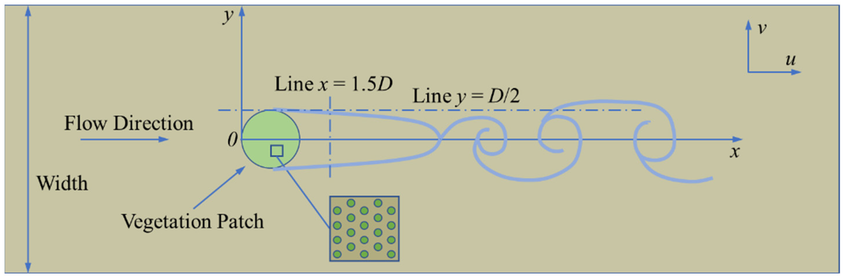
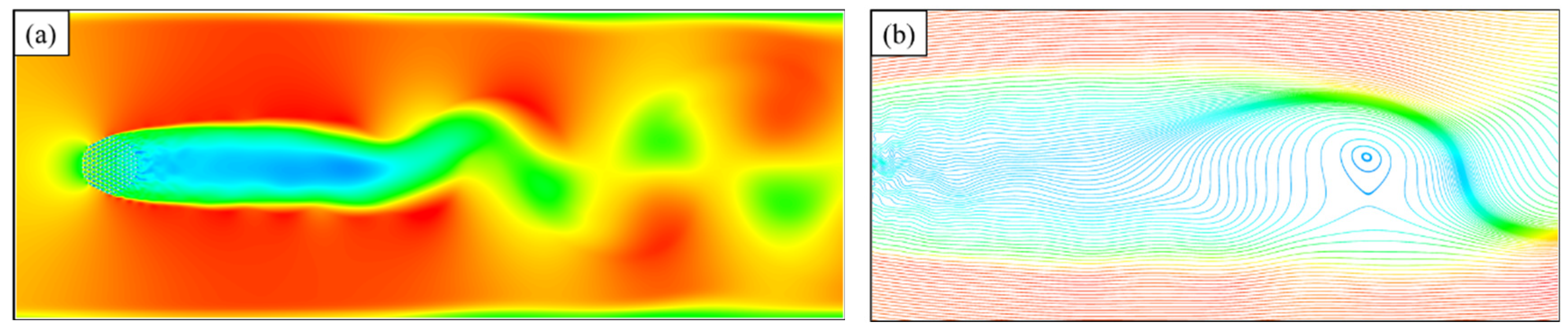
Figure 5 shows the wake behind the vegetation patch, the shear flow on both sides of the wake, and the special flow velocity distribution due to the von-Kármán vortex street behind the stable wake section. The smooth streamline diagram of flow after an emerged vegetation patch arranged in the channel is provided in Figure 5.
Represented by L, the total wake segment length spans from the downstream edge of the vegetation patch to the location at the centerline, where the velocity recovery rate is reduced to 0.1, i.e.,
u ¯ / U x / D < 0.1
The wake segment is composed of a stable wake segment and a wake recovery segment. The stable wake segment is an area between the downstream edge of the vegetation patch and the formation location of the vortex street, and its length is represented by L1. The length of the wake recovery segment is represented by L2,   L 2 = L L 1 [3].
In the preliminary analysis, all six turbulence models were able to make predictions of the interaction between an emerged vegetation patch and the water flow. The simulation results of the six turbulence models were all consistent with the physical characteristics derived from the experiments of Zong and Nepf [3]. However, differences in results were observed for each numerical simulation, and all of the model results exhibited different degrees of deviation from the experimental results. Among them, the RSM model showed the most unsatisfactory performance in predicting the vegetation patch wake.

3.1. Comparative Analysis of Mean Velocity Profile and Wake Segment Simulation

Numerical simulation data of the six turbulence models were collected. The data at the lines y = 0 and y = 0.11 m shown in Figure 1 were statistically analyzed. Figure 6 and Figure 7 depict the time-averaged velocity distribution of each example at the two lines for each simulation case in comparison with the experimental data of Zong and Nepf [3].
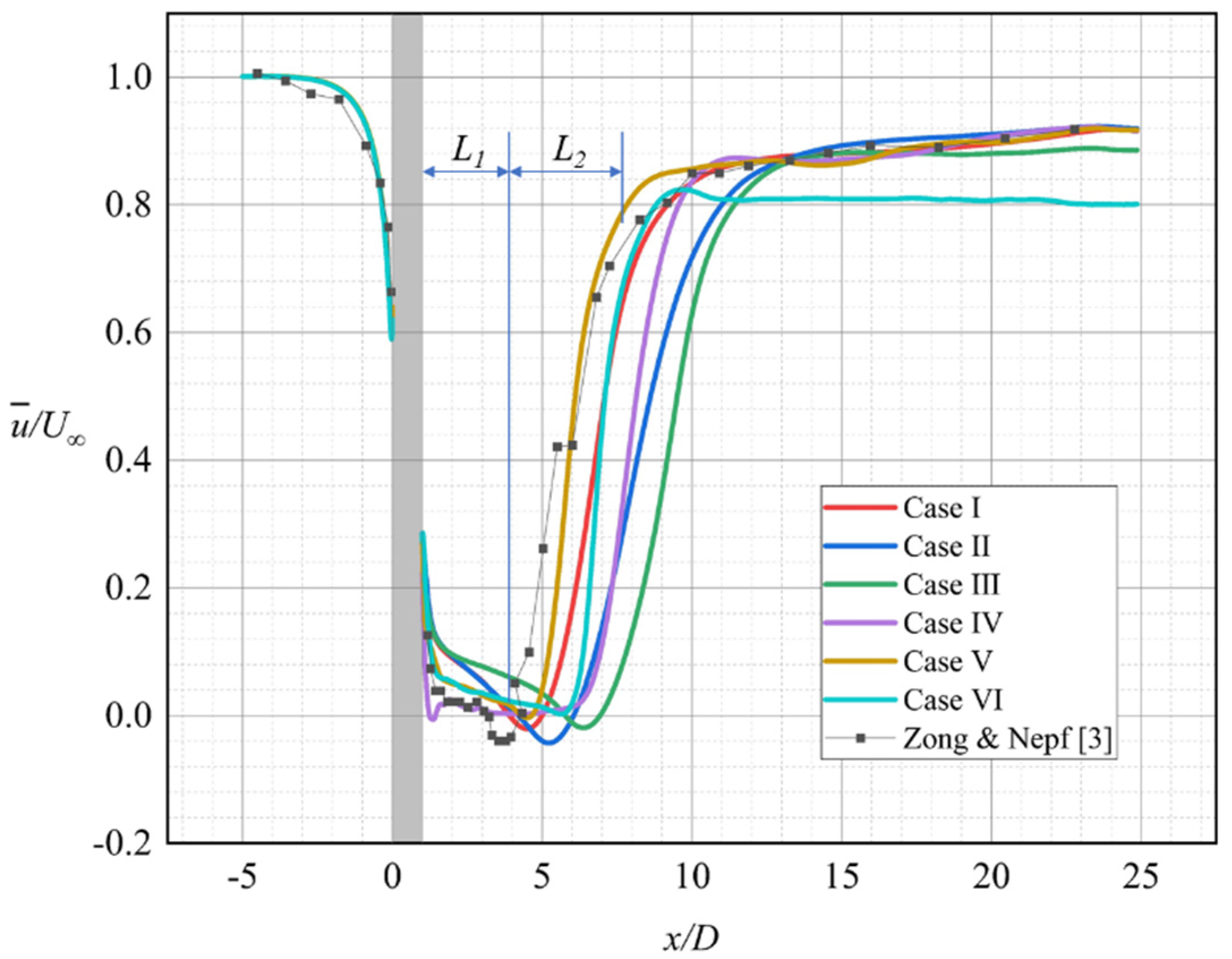
Figure 6 depicts the time-averaged longitudinal flow velocity distribution of the six turbulence models at the wake centerline. On the basis of the experimental results of Zong and Nepf [3], the results of six numerical simulation examples were consistent with the experimental physical characteristics of laboratory experiments. All six turbulence models were able to simulate reasonable longitudinal mean flow velocity distributions at the centerline, including the stable wake segment and wake recovery segment. The values are shown in Figure 8. Figure 6 illustrates that the predictions of the numerical simulations deviated from the experimental data. Case V simulated by the SST k-ω model had the simulation results with the least overall deviation from the experimental data. The other five turbulence models had great deviations at different locations. In Figure 6, L1 and L2, respectively, mark the distribution of the mean flow velocity u ¯ in the steady wake segment and the wake recovery segment from the experimental data of Zong and Nepf [3]. The flow velocities in the wake stable segment L1 simulated by the three turbulence models of the k-ε series were remarkably larger than those of the experimental data. In addition to the SST k-ω model, the other five turbulence models predicted that the wake recovery segment was highly downstream. Only the realizable k-ε model and RSM model poorly predicted the distribution and magnitude of the mean flow velocity u ¯ after the wake. Among the six turbulence models, the worst prediction results were provided by the RSM model. The simulation results of the RSM model were unsatisfactory in the wake segment, and the flow velocity prediction after the wake section highly differed from that in the experimental data. The relative velocity of the experimental data at x = 23D is about 0.9, while about 0.8 for RSM. Meanwhile, the numerical simulation results of the standard k-ε model were better than those of the RNG k-ε model and realizable k-ε model. This finding is unexpected because the realizable k-ε model shows better performance than the standard k-ε model in most previous numerical simulation examples.
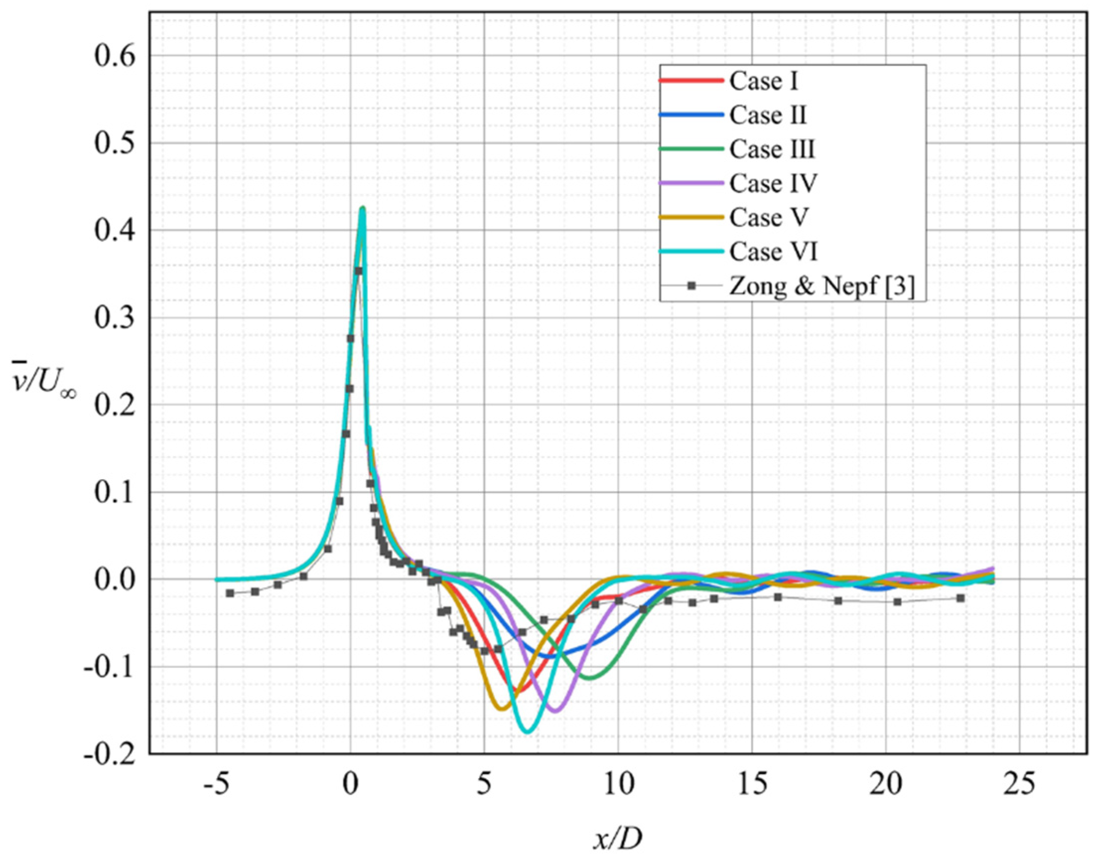
Figure 7 depicts the numerical simulations results of the transverse mean flow velocity v ¯ profiles at the line y = D/2. Although the six turbulence models were able to correctly represent the physical characteristics consistent with the experiments of Zong and Nepf [3], they showed varying degrees of deviation in specific values. The minimum position of the transverse mean velocity v ¯ at the line y = D/2 was more downstream than that in the experimental data. Among the six turbulence models, the SST k-ω model simulated the most consistent results with the experimental data but underestimated the minimum value of v ¯ . The minimum value of v ¯ predicted by the RNG k-ε model was consistent with the experimental data of Zong and Nepf [3], but the location of the minimum value was more downstream. A high recovery rate of the minimum value is associated with a fast shear flow on both sides of the vegetation patch and a short wake recovery segment. On this basis, the predicted length of wake recovery segment by the RSM model was too small.
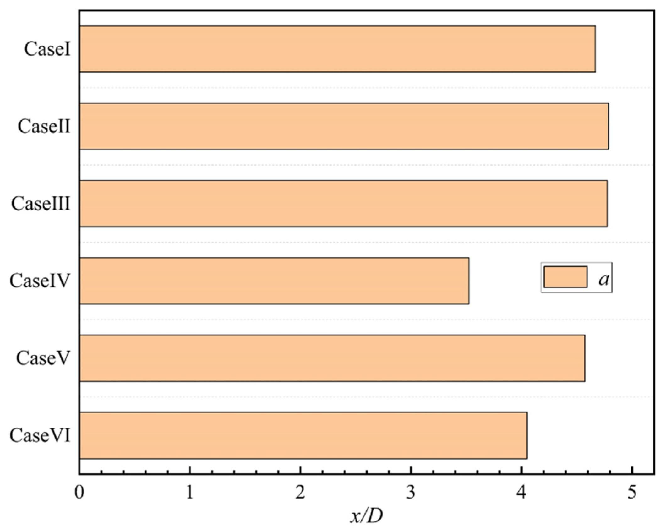
Figure 8 summarizes the numerical simulation results of the wake segment length for the six numerical cases. All of the turbulence models predicted greater length L for the emerged vegetation patch compared with that in Zong and Nepf experiments [3] (about 10% to 47.8% excess of the experimental data), except for the prediction results of the SST k-ω model that were in good agreement with the experimental data. Among them, the realizable k-ε model predicted the highest L value compared to the experimental data, about 47.8% of the experimental data. For the stable wake segment length L1, the six turbulence models predicted longer values than that obtained from the experiments (about 20.7% to 93.1% excess of the experimental data). For the wake recovery segment length L2, the simulation results of the standard k-ε model were the most consistent with the experimental data (the difference is less than 3% of the experimental data). The predicted L2 values by the RNG k-ε model and realizable k-ε model were larger than the experimental values, and the predictions of the standard k-ω model, SST k-ω model, and RSM model were smaller.

3.2. Simulation Results of Flow Field after Vegetation Patch

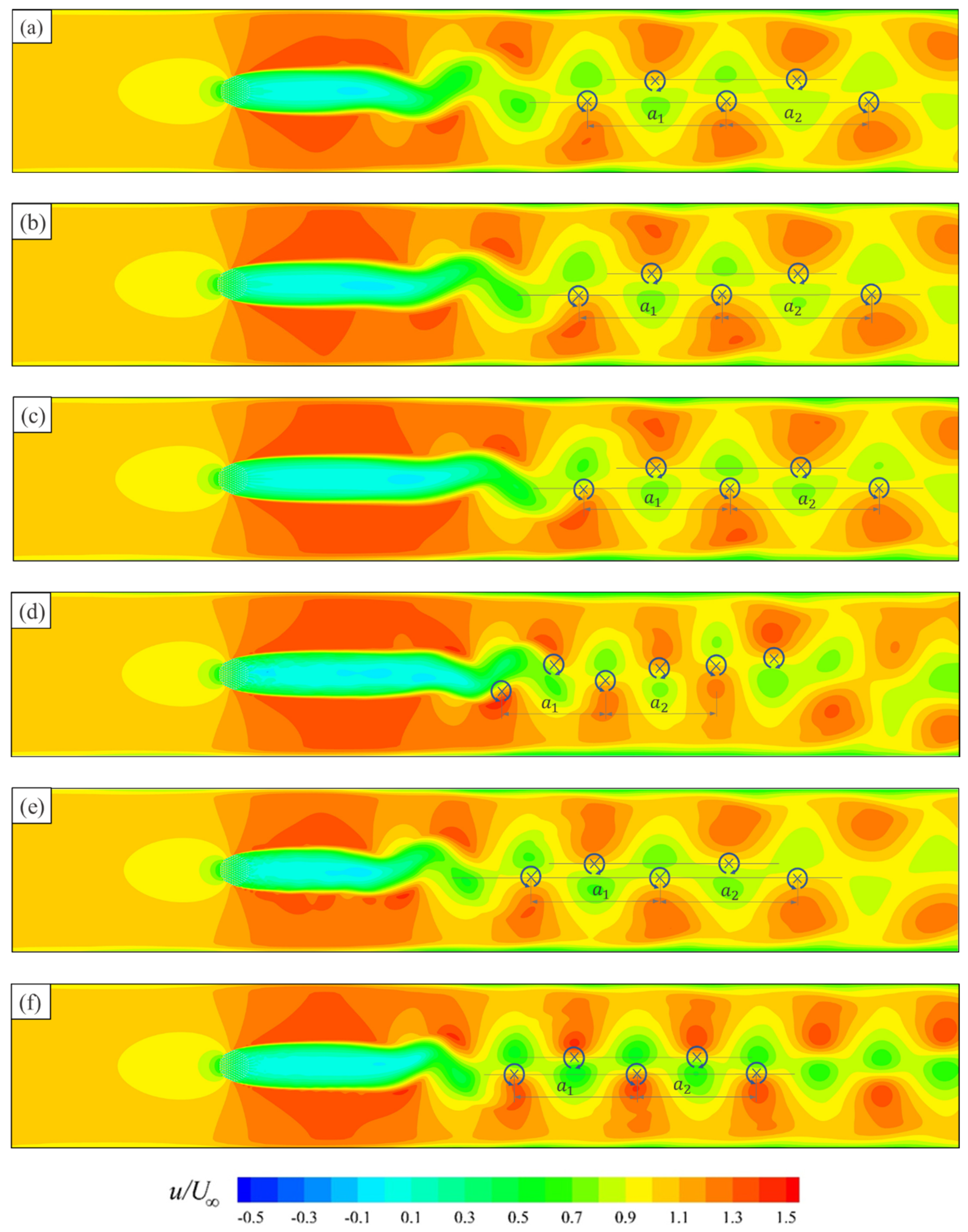
Figure 9 shows the transient velocity distribution contours simulated by the six turbulence models and colored by the longitudinal flow velocity u. The obstructive effect of an emerged vegetation patch led to the formation of a low flow velocity segment (the wake) behind the vegetation patch, and the flow velocity on both sides of the vegetation patch was increased by the squeezing effect, generating shear layers. The shear layers gradually developed and widened with the flow until the shear layers on both sides interacted, forming Kármán vortex street after the wake region. The distribution of the Kármán vortices street in the contours for each case is marked in Figure 9. These positions were confirmed based on the flow velocity vector diagram and the x values for which v(x) takes the extremum. The comparison indicates that all of the applied turbulence models were able to make predictions for the two vortex sheets behind the wake. In the calculation domain, all turbulence models did not capture the breakdown of the main vortex street, except the standard k-ω model. The simulation by the standard k-ω model demonstrated the instability and intermixing of the two vortex sheets behind the wake. Compared with that predicted by the standard k-ω model, the main vortex street lengths after the wake predicted by the standard k-ε model, RNG k-ε model, realizable k-ε model, SST k-ω model, and RSM model simulations were larger and more stable. The distances between neighboring vortices at the same vortex sheet of the main vortex street are represented by a 1 and a 2 . Here a 1 and a 2 are consecutive, and a 1 is closer to the upstream. In other words, a 1 and a 2 include three consecutive vortices on the same vortex sheet.
a 1 and a 2 were averaged to represent the wavelength of the main vortex street for each turbulence model prediction result.
a = a 1 + a 2 2
Figure 10 illustrates the comparison of the numerical simulation results of six turbulence models for the wavelength of the main vortex street. Figure 10 illustrates the wavelength of the main vortex street of the numerical simulation results presented in Figure 9.
The standard k-ε model, RNG k-ε model, and realizable k-ε model produced relatively consistent prediction results of the main vortex street wavelength after the wake. The difference between the prediction results of the SST k-ω model and the standard k-ε model was extremely small because the calculation of the far-field region of the SST k-ω model was consistent with that of the standard k-ε model. According to the prediction results of the standard k-ω model, its predicted main vortex street wavelength was significantly small. When the wavelength decreases, the velocity fluctuation frequency of the main vortex street increases, corresponding to the smaller vortex shedding frequency behind the vegetation patch.

3.3. Comparative Analysis of Longitudinal Outflow Intensity

The emerged vegetation patch are porous areas, and some of the water flow can form outflows on the sides and back of the patch through the gaps between the plants. The longitudinal outflow in an emerged vegetation patch will form a stable wake segment, a wake recovery section, and a Kármán vortex street behind the vegetation patch. The longitudinal outflow intensity of an emerged vegetation patch is closely related to the diameter D of the vegetation patch and the vegetation density Φ [9]. Therefore, the longitudinal outflow of the simulation results of the six turbulence models can be compared by comparing the transverse distribution of the longitudinal mean flow velocity u ¯ behind the vegetation patch. It should be noted that the instantaneous longitudinal velocity distributions in 
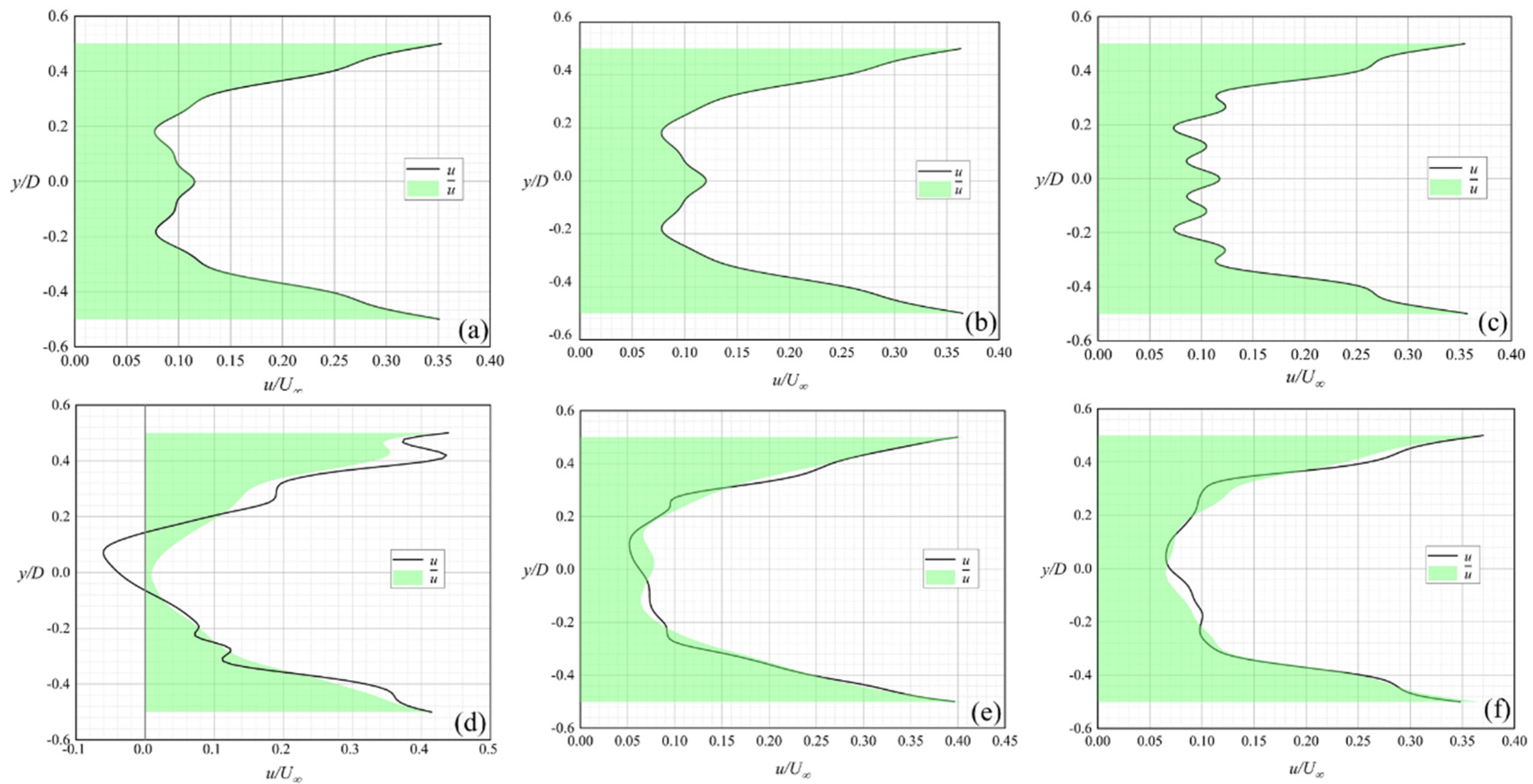
Figure 11 are not at the same time, and there is no need to compare the instantaneous longitudinal velocity distributions of the six turbulence models. Figure 11 depicts the longitudinal outflow from the numerical simulation results under the six turbulence models. The distributions of flow velocity u and u ¯ at line x = 1.5D in the stable wake segment were collected, and the position of the transverse line is marked in Figure 1. The dimensionless distributions of the mean longitudinal velocity u ¯ and the transient longitudinal velocity u simulated by the six turbulence models were compared, as shown in Figure 11.
Given that the shear flow on both sides of the emerged vegetation patch gradually developed along the flow direction, the mean flow velocity u ¯ and transient flow velocity u located near y = ± 0.5 D were larger than the flow velocity near the centerline but were not affected by the development of shear flow. Figure 11a,b shows the good consistency between the simulations of the mean longitudinal outflow at x = 1.5D by the standard k-ε model and the RNG k-ε model. The large overlap between the distributions of the mean flow velocity u ¯ and the transient flow velocity u in Figure 11a–c indicated the stability in time of the steady wake segment, simulated by the standard k-ε model, RNG k-ε model, and realizable k-ε model. The multiple maximum and minimum values of longitudinal flow velocities in Figure 11c revealed that the turbulence in the stable wake segment simulated by the realizable k-ε model was extremely weak, and the interaction between the longitudinal outflows behind the porous region occurred in the further downstream. In Figure 11d, the distribution of transient velocity u had negative values, indicating that the turbulence in the stable wake segment predicted by the standard k-ω model was intensive, and reflux can be observed in the segment. The distributions of the mean flow velocity u ¯ illustrated in Figure 11d–f did not match with the distribution of the transient flow velocity u. This finding indicates that the longitudinal outflow fluctuated in time at line x = 1.5D simulated by the standard k-ω model, SST k-ω model, and RSM model. Therefore, different degrees of turbulence existed in the stable wake segment predicted by these three turbulence models.

3.4. Computational expenses

In the application of numerical simulation, an important concern is the calculation cost. Usually, fast and economical methods will be more widely adopted. For this reason, the calculation demands of the six models relative to the standard k-e model simulation are given in Table 5. It should be noted that all of the simulations were intentionally conducted on the same computer.
It is worth mentioning that the SST k- ω model obtained the most consistent fluency characteristics with the experimental data of Zong and Nepf [3] in Section 3.1. In Table 5, the relative iteration time of SST k- ω is also the smallest, which means the lowest computational expense. In other words, the SST k- ω model is relatively accurate and efficient under the current research background and conditions.

4. Conclusions

This work mainly investigates the interaction between an emerged vegetation patch and water flow in a straight channel by 2D CFD. A comparative analysis is also conducted on the simulation results of different turbulence models. The interaction between vegetation patches and water flow is extremely sensitive to the diameter and density of the vegetation patch, so the current results are only strictly valid for the current situation [2]. All six turbulence models currently selected are able to make reasonable simulations and predictions of the flow field with different degrees of accuracy.
In the computational domain, all six turbulence models are able to simulate the shear flow on both sides of the emerged vegetation patch, the wake, and the Kármán vortex street behind the patch. The standard k-ε model is able to simulate reasonable and accurate simulation predictions for the current range of flow field characteristics. Moreover, it is better than the RNG k-ε model and realizable k-ε model in terms of consistency with the experimental data of Zong and Nepf [3]. The SST k-ω model has the best agreement with the experimental data in stimulating the interaction between an emerged vegetation patch and water flow in a straight channel, including the mean longitudinal velocity distribution at the central line, the transverse mean velocity distribution at the line y = D/2, length of the wake segment. The standard k-ω model and the RSM do not perform well. From the simulation results, the turbulence intensity of RSM, the standard k-ω model, and the SST k-ω model is stronger than that of the standard k-ε model, RNG k-ε model, and realizable k-ε model. For the prediction of turbulent structure around rigid emerged vegetation by 2D numerical simulation, the SST k-ω model can achieve better results than the standard k-ε model, RNG k-ε model, realizable k-ε model, standard k-ω model, and Reynolds stress model (RSM). In addition, the SST k-ω model has the lowest computational expense in current research.

Author Contributions

Conceptualization, W.H. and S.Y.; methodology, W.H., M.L. and S.Y.; validation, H.D. and S.Y.; visualization, Y.Z. and S.Y.; supervision, W.H.; writing—original draft preparation, S.Y.; writing—review and editing, W.H., M.L. and S.Y. All authors have read and agreed to the published version of the manuscript.

Funding

This work was supported by the National Natural Science Foundation of China [grant numbers 52020105006, 12272281, 11872285].

Data Availability Statement

Data are contained within the article.

Conflicts of Interest

The authors declare no conflict of interest.

References

  1. Huai, W.; Li, S.; Katul, G.G.; Liu, M.; Yang, Z. Flow dynamics and sediment transport in vegetated rivers: A review. J. Hydrodyn. 2021, 33, 400–420. [Google Scholar] [CrossRef]
  2. Wang, C.; Zheng, S.; Wang, P.; Hou, J. Interactions between vegetation, water flow and sediment transport: A review. J. Hydrodyn. 2015, 27, 24–37. [Google Scholar] [CrossRef]
  3. Zong, L.; Nepf, H. Vortex development behind a finite porous obstruction in a channel. J. Fluid Mech. 2012, 691, 368–391. [Google Scholar] [CrossRef]
  4. Liu, M.; Huai, W.; Yang, Z.; Zeng, Y. A genetic programming-based model for drag coefficient of emergent vegetation in open channel flows. Adv. Water Resour. 2020, 140, 103582. [Google Scholar] [CrossRef]
  5. Caroppi, G.; Västilä, K.; Järvelä, J.; Lee, C.; Ji, U.; Kim, H.S.; Kim, S. Flow and wake characteristics associated with riparian vegetation patches: Results from field-scale experiments. Hydrol. Process. 2022, 36, e14506. [Google Scholar] [CrossRef]
  6. Huai, W.; Zhang, J.; Katul, G.G.; Cheng, Y.; Tang, X.; Wang, W. The structure of turbulent flow through submerged flexible vegetation. J. Hydrodyn. 2019, 31, 274–292. [Google Scholar] [CrossRef]
  7. Yu, Z.; Shan, Y.; Liu, C.; Liu, X. Wake flow and vortex structures behind emergent vegetation patches elongated in the longitudinal direction. J. Hydrodyn. 2021, 33, 1148–1161. [Google Scholar] [CrossRef]
  8. White, B.L.; Nepf, H.M. Shear instability and coherent structures in shallow flow adjacent to a porous layer. J. Fluid Mech. 2007, 593, 1–32. [Google Scholar] [CrossRef]
  9. Liu, M.; Huai, W.; Ji, B. Characteristics of the flow structures through and around a submerged canopy patch. Phys. Fluids 2021, 33, 035144. [Google Scholar] [CrossRef]
  10. Liu, M.; Huai, W.; Ji, B.; Han, P. Numerical study on the drag characteristics of rigid submerged vegetation patches. Phys. Fluids 2021, 33, 085123. [Google Scholar] [CrossRef]
  11. Liu, Z.; Chen, Y.; Wu, Y.; Wang, W.; Li, L. Simulation of exchange flow between open water and floating vegetation using a modified RNG k-ε turbulence model. Environ. Fluid Mech. 2017, 17, 355–372. [Google Scholar] [CrossRef]
  12. Liu, M.; Yang, Z.; Ji, B.; Huai, W.; Tang, H. Flow dynamics in lateral vegetation cavities constructed by an array of emergent vegetation patches along the open-channel bank. Phys. Fluids 2022, 34, 035122. [Google Scholar] [CrossRef]
  13. Anjum, N.; Ghani, U.; Pasha, G.A.; Latif, A.; Sultan, T.; Ali, S. To Investigate the Flow Structure of Discontinuous Vegetation Patches of Two Vertically Different Layers in an Open Channel. Water 2018, 10, 75. [Google Scholar] [CrossRef]
  14. Anjum, N.; Tanaka, N. Investigating the turbulent flow behaviour through partially distributed discontinuous rigid vegetation in an open channel. River Res. Appl. 2020, 36, 1701–1716. [Google Scholar] [CrossRef]
  15. Qu, J.; Yu, J. A numerical modelling of flows in an open channel with emergent vegetation. J. Hydraul. Res. 2021, 59, 250–262. [Google Scholar] [CrossRef]
  16. Zhan, J.; Hu, W.; Cai, W.; Ye-Jun, Y.; Li, C. Numerical simulation of flow through circular array of cylinders using porous media approach with non-constant local inertial resistance coefficient. J. Hydrodyn. 2017, 29, 168–171. [Google Scholar] [CrossRef]
  17. Yamasaki, T.N.; de Lima, H.S.; Silva, D.F.; Preza, C.G.D.A.; Janzen, J.G.; Nepf, H.M. From patch to channel scale: The evolution of emergent vegetation in a channel. Adv. Water Resour. 2019, 129, 131–145. [Google Scholar] [CrossRef]
  18. Zhu, Z.; Yang, Z.; Huai, W.; Wang, H.; Li, D.; Fan, Y. Growth-decay model of vegetation based on hydrodynamics and simulation on vegetation evolution in the channel. Ecol. Indic. 2020, 119, 106857. [Google Scholar] [CrossRef]
  19. Li, D.; Huai, W.; Liu, M. Investigation of the flow characteristics with one-line emergent canopy patches in open channel. J. Hydrol. 2020, 590, 125248. [Google Scholar] [CrossRef]
  20. Farhadi, A.; Mayrhofer, A.; Tritthart, M.; Glas, M.; Habersack, H. Accuracy and comparison of standard k-ε with two variants of k-ω turbulence models in fluvial applications. Eng. Appl. Com Fluid 2018, 12, 216–235. [Google Scholar]
  21. Shaheed, R.; Mohammadian, A.; Gildeh, H.K. A comparison of standard k–ε and realizable k–ε turbulence models in curved and confluent channels. Environ. Fluid Mech. 2019, 19, 543–568. [Google Scholar] [CrossRef]
  22. de Lima, H.S.; Janzen, J.G.; Nepf, H.M. Flow patterns around two neighboring patches of emergent vegetation and possible implications for deposition and vegetation growth. Environ. Fluid Mech. 2015, 15, 881–898. [Google Scholar] [CrossRef]
  23. Brito, M.; Fernandes, J.; Leal, J.B. Porous media approach for RANS simulation of compound open-channel flows with submerged vegetated floodplains. Environ. Fluid Mech. 2016, 16, 1247–1266. [Google Scholar] [CrossRef]
  24. Versteeg, H.; Malalasekera, W. An Introduction to Computational Fluid Dynamics: The Finite Volume Method, 2nd ed.; Pearson: London, UK, 2007. [Google Scholar]
  25. Ferziger, J.H.; Peric, M.; Leonard, A. Computational Methods for Fluid Dynamics. Phys. Today 1997, 50, 80–84. [Google Scholar] [CrossRef]
  26. Xiao, H.; Cinnella, P. Quantification of model uncertainty in RANS simulations: A review. Prog. Aeros. Sci. 2019, 108, 1–31. [Google Scholar] [CrossRef]
  27. Launder, B.E.; Spalding, D.B. Lectures in Mathematical Model of Turbulence; Academic Press: Cambridge, MA, USA, 1972. [Google Scholar]
  28. Ben Ramoul, L.; Korichi, A.; Popa, C.; Zaidi, H.; Polidori, G. Numerical study of flow characteristics and pollutant dispersion using three RANS turbulence closure models. Environ. Fluid Mech. 2019, 19, 379–400. [Google Scholar] [CrossRef]
  29. Yakhot, V.; Orszag, S.A. Renormalization group analysis of turbulence. I. Basic theory. J. Sci. Comput. 1986, 1, 3–51. [Google Scholar] [CrossRef]
  30. Koutsourakis, N.; Bartzis, J.G.; Markatos, N.C. Evaluation of Reynolds stress, k-ε and RNG k-ε turbulence models in street canyon flows using various experimental datasets. Environ. Fluid Mech. 2012, 12, 379–403. [Google Scholar] [CrossRef]
  31. Bulat, M.; Bulat, P. Comparison of Turbulence Models in the Calculation of Supersonic Separated Flows. World Appl. Sci. J. 2013, 27, 1263–1266. [Google Scholar]
  32. Shih, T.H.; Liou, W.W.; Shabbir, A.; Yang, Z.; Jiang, Z. A new k-e eddy viscosity model for high Reynolds number turbulent flows. Comput. Fluids 1995, 24, 227–238. [Google Scholar] [CrossRef]
  33. Duan, Y.; Jackson, C.; Eaton, M.D.; Bluck, M.J. An assessment of eddy viscosity models on predicting performance parameters of valves. Nucl. Eng. Des. 2019, 342, 60–77. [Google Scholar] [CrossRef]
  34. Wilcox, D.C. Turbulence Modeling for CFD; DCW Industries Inc.: La Canada, CA, USA, 2006. [Google Scholar]
  35. Launder, B.E.; Reece, G.J.; Rodi, W. Progress in the development of a Reynolds-stress turbulence closure. J. Fluid Mech. 1975, 68, 537–566. [Google Scholar] [CrossRef] [Green Version]
  36. Wilcox, D.C. Formulation of the k-w Turbulence Model Revisited. AIAA J. 2008, 46, 2823–2838. [Google Scholar] [CrossRef]
  37. Menter, F.R. Two-equation eddy-viscosity turbulence models for engineering applications. AIAA J. 1994, 32, 1598–1605. [Google Scholar] [CrossRef]
  38. Menter, F.R. Review of the shear-stress transport turbulence model experience from an industrial perspective. Int. J. Comput. Fluid Dyn. 2009, 23, 305–316. [Google Scholar] [CrossRef]
  39. Karbon, M.; Sleiti, A.K. Turbulence Modeling Using Z-F Model and RSM for Flow Analysis in Z-SHAPE Ducts. J. Eng. 2020, 2020, 1–10. [Google Scholar] [CrossRef]
  40. Gibson, M.M.; Launder, B.E. Ground effects on pressure fluctuations in the atmospheric boundary layer. J. Fluid Mech. 1978, 86, 491–511. [Google Scholar] [CrossRef]
  41. Altaç, Z.; Uğurlubilek, N. Assessment of turbulence models in natural convection from two- and three-dimensional rectangular enclosures. Int. J. Therm. Sci. 2016, 107, 237–246. [Google Scholar] [CrossRef]
  42. Maly, M.; Slama, J.; Cejpek, O.; Jedelsky, J. Searching for a Numerical Model for Prediction of Pressure-Swirl Atomizer Internal Flow. Appl. Sci. 2022, 12, 6357. [Google Scholar] [CrossRef]
  43. Van Doormaal, J.; Raithby, G.D. Enhancements of the Simple Method for Predicting Incompressible Fluid Flows. Numer. Heat Transf. Part. B Fundam. 1984, 7, 147–163. [Google Scholar] [CrossRef]
Figure 1. Top view of the numerical simulation arrangement. An emerged vegetation patch is arranged at the central line of a rectangular channel.
Water 14 02873 g001
Figure 2. Computational grid for the cases of D = 22 cm and ϕ = 0.1: (a) a close view of the wake area grid, (b) a detailed view of the grid near the circular hole, and (c) a feature view of the grid near the wake behind the vegetation patch.
Water 14 02873 g002
Figure 3. The simulation results of case V, case VII, and case VIII are compared with those of Zong and Nepf [3]. The diameter of the vegetation patch is 22 cm, and the data in the figure are the centerline (y = 0) longitudinal mean velocity ( u ¯ ) distribution. The gray part indicates the internal area of vegetation patches.
Water 14 02873 g003
Figure 4. The simulation results of case V, case VIII, and case X are compared with those of Zong and Nepf [3]. The data in the figure is the centerline (y = 0) longitudinal mean velocity ( u ¯ ) distribution. The gray part indicates the internal area of vegetation patches.
Water 14 02873 g004
Figure 5. (a) Contour of longitudinal velocity u distribution of water flow obstructed by a vegetation patch, and (b) streamlines colored by velocity u near the stable wake segment; both are the numerical simulation results of SST k- ω turbulence model.
Water 14 02873 g005
Figure 6. The longitudinal flow profiles simulated by six turbulence models are illustrated in comparison with the experimental results of Zong and Nepf ( Φ = 0.1, D = 22 cm) [3], where the longitudinal mean velocity u ¯ is measured at the centerline, y = 0. The gray part indicates the internal area of vegetation patches.
Water 14 02873 g006
Figure 7. Transverse velocity v ¯ is measured at line y = D/2; the black dot plot in the figure is the experimental data of Zong and Nepf ( Φ = 0.1, D = 22 cm) [3].
Water 14 02873 g007
Figure 8. The lengths of the wake segments obtained from the cases and experiments of Zong and Nepf are illustrated [3]; blue indicates the stable wake segment, and green indicates the wake recovery segment; the blue and green dashed line indicates the L1 and L2 of experiments. The gray part indicates the internal area of vegetation patches.
Water 14 02873 g008
Figure 9. Contours of instantaneous velocity distribution for Φ = 0.1 and D = 22 cm colored by velocity u. (a) case I, (b) case II, (c) case III, (d) case IV, (e) case V, and (f) case VI. Arrows indicate the direction of the vortex rotation.
Water 14 02873 g009
Figure 10. Wavelength comparison of main vortex street for six cases.
Water 14 02873 g010
Figure 11. The black curve indicates the transient longitudinal flow velocity u distribution, and the green area indicates the cumulative plot of the mean longitudinal flow velocity u ¯ to the line u ¯ / U = 0. (a) case I, (b) case II, (c) case III, (d) case IV, (e) case V, and (f) case VI.
Water 14 02873 g011
Table 1. Information of numerical simulation cases. Geometric and hydrodynamic parameters are given.
Case Φ a   ( cm 1 ) D (cm)D (cm)U (cm/s) R e d Turbulence ModelTime Step (s)Grid Cells (k)
I0.10.2220.69.8588Standard k-ε0.01349
II0.10.2220.69.8588RNG k-ε0.01349
III0.10.2220.69.8588Realizable k-ε0.01349
IV0.10.2220.69.8588Standard k-ω0.01349
V0.10.2220.69.8588SST k-ω0.01349
VI0.10.2220.69.8588RSM0.01349
VII0.10.2220.69.8588SST k-ω0.01258
VIII0.10.2220.69.8588SST k-ω0.01489
IX0.10.2220.69.8588SST k-ω0.05349
X0.10.2220.69.8588SST k-ω0.005349
Table 2. Details of the cases for model validation.
Model ValidationTurbulence ModelTime Size (s)Grid Cells(k)
Grid independence validationCase VIISST k-ω0.01258
Case VSST k-ω0.01349
Case VIIISST k-ω0.01489
Time step independence validationCase IXSST k-ω0.05349
Case VSST k-ω0.01349
Case XSST k-ω0.005349
Table 3. Some results of cases V, VII, and VIII for grid independence validation, where L 1 is defined in Section 3.
CaseGlobal Maximum Mean Velocity (cm/s)Maximum Longitudinal Mean Velocity (cm/s) L 1   ( D )
VII13.0802213.075094.6
V13.0797413.076164.5
VIII13.0776713.075934.5
Table 4. Some results of cases V, IX, and X for time step independence validation, where L 1 is defined in Section 3.
CaseGlobal Maximum Mean Velocity (cm/s)Maximum Longitudinal Mean Velocity (cm/s) L 1   ( D )
IX13.0587813.054894.9
V13.0797413.076164.5
X13.0801213.084744.5
Table 5. Computational expenses of the six turbulence models.
CaseTurbulence ModelGrid Cells (k)Time Step (s)Relative Iteration Time
IStandard k-ε3490.11.00
IIRNG k-ε3490.11.07
IIIRealizable k-ε3490.11.06
IVStandard k-ω3490.11.46
VSST k-ω3490.10.87
VIRSM3490.11.21
Publisher’s Note: MDPI stays neutral with regard to jurisdictional claims in published maps and institutional affiliations.

