
Development of a Temperature-Based Model Using Machine Learning Algorithms for the Projection of Evapotranspiration of Peninsular Malaysia

 ,
,  ,
,  and
and 
Abstract
:1. Introduction
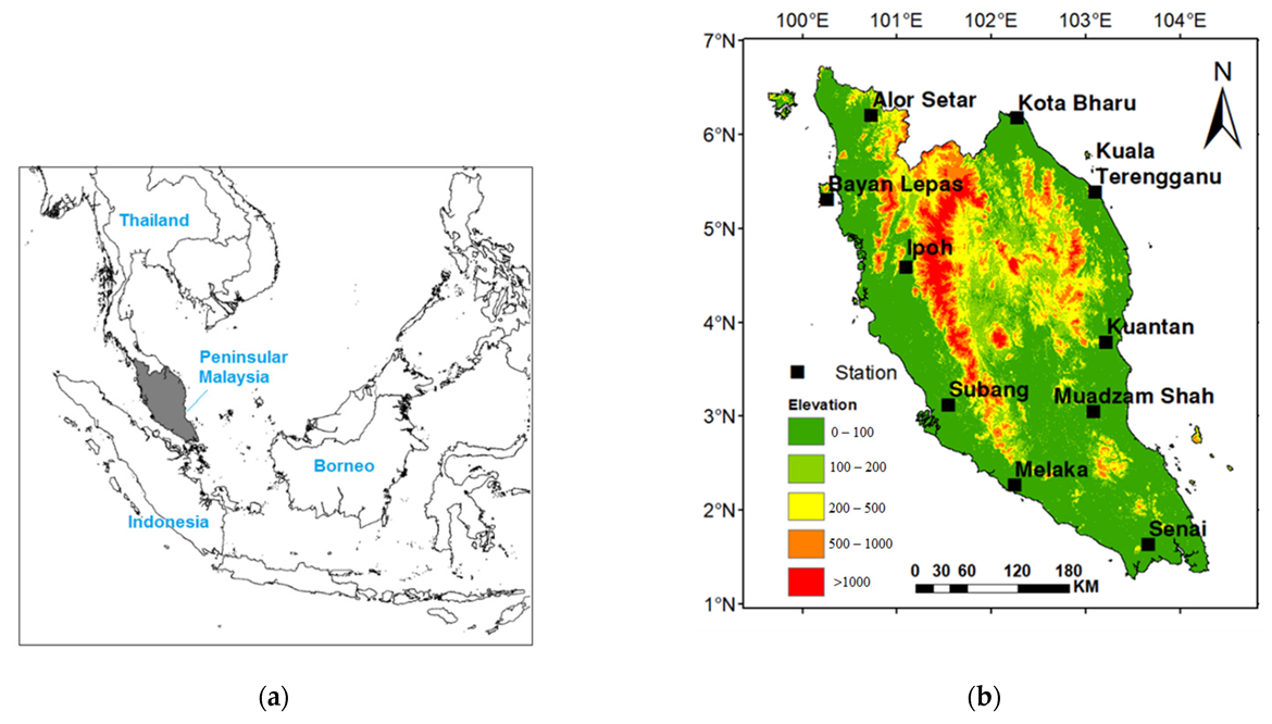
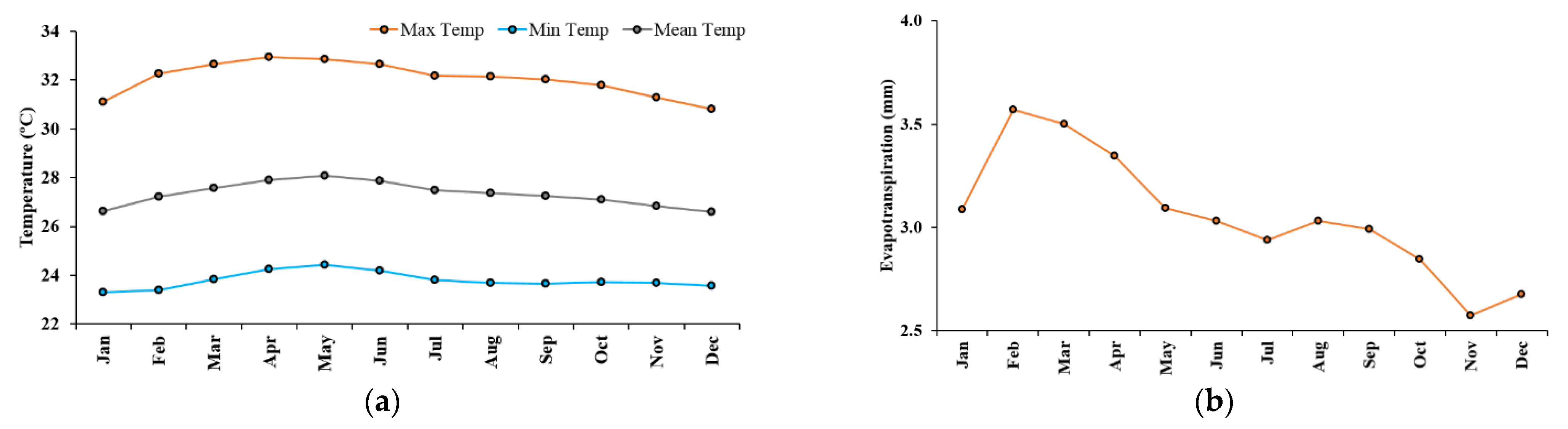
2. Study Area
3. Data
4. Methodology
- Gene expression programming (GEP) was used to generate a temperature-based empirical equation for the estimation of ET for peninsular Malaysia
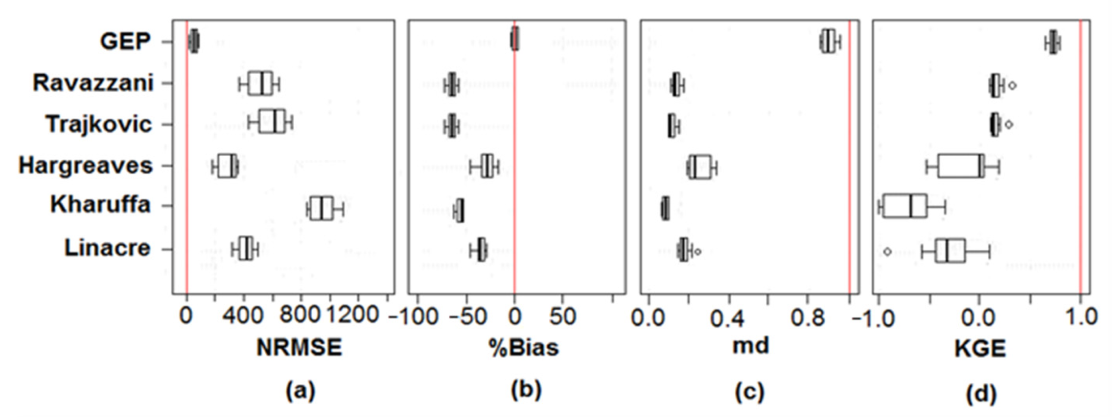
- The accuracy of the newly developed empirical model was assessed by comparing its performance with the existing temperature-based empirical methods
- GCMs were used to downscale and project temperatures at the study locations.
- The newly developed GEP ET model was used to project the ET of Peninsular Malaysia from the GCM projected temperature
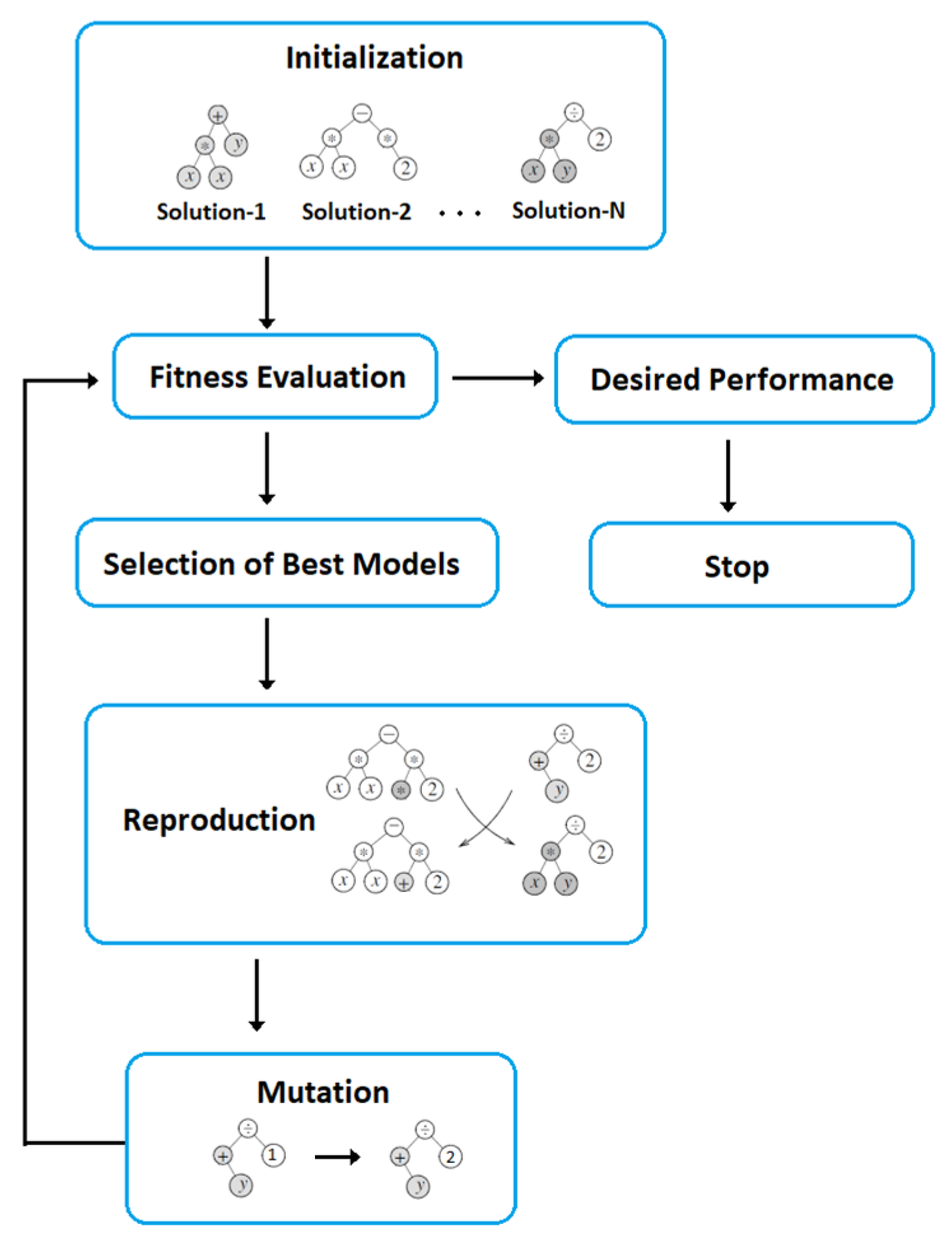
4.1. Gene Expression Programming (GEP)
- Selection of fitness function or a set of fitness functions. The Nash–Sutcliff Efficiency (NSE) was considered for the fitness function.
- Selection of a set of terminals and a set of functions. The inputs were selected according to their influence on ET.
- Creation of chromosomes from the selected terminals and functions.
- Setting the chromosomal architecture.
- Selection of the linking function.
- Selection of genetic operators.
4.2. Temperature-Based ET Methods
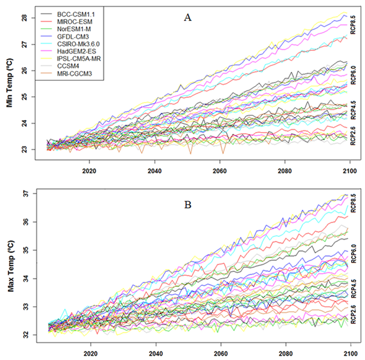
4.3. Temperature Downscaling and Projections
5. Results & Discussion
5.1. Development of Temperature-Based ET Equations Using GEP
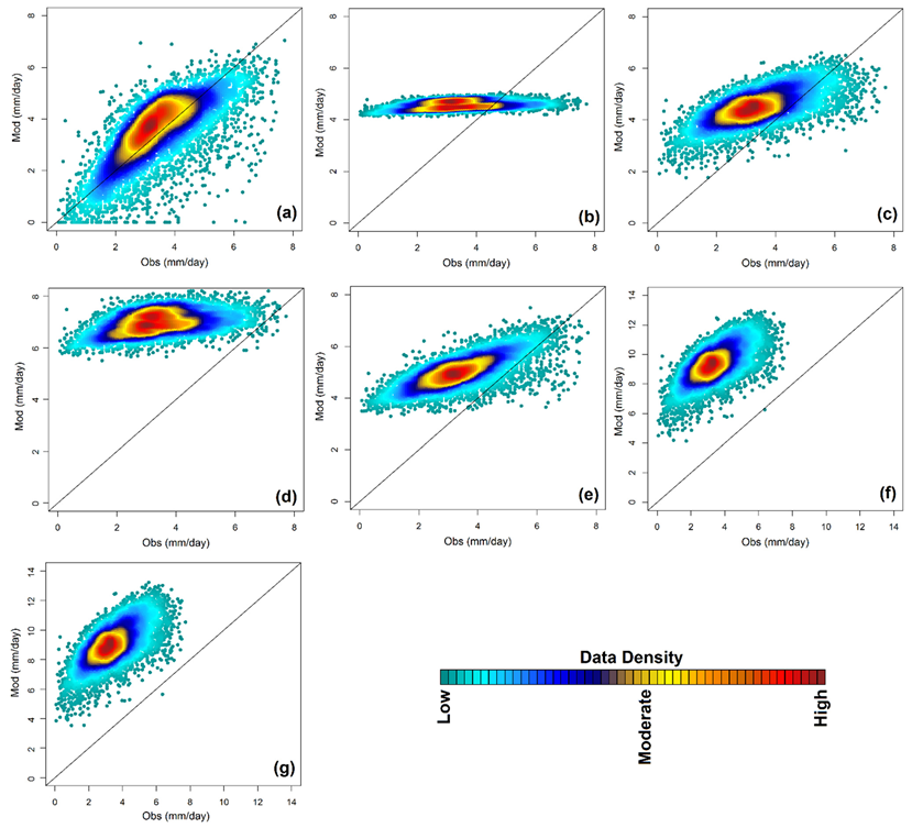
5.2. Performance Evaluation of GEP ET Equations
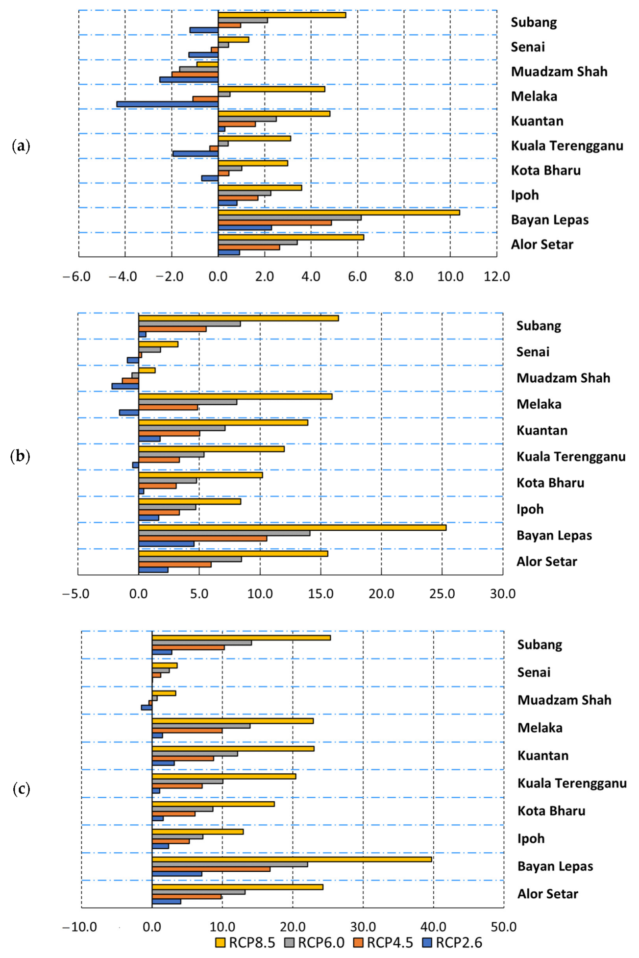
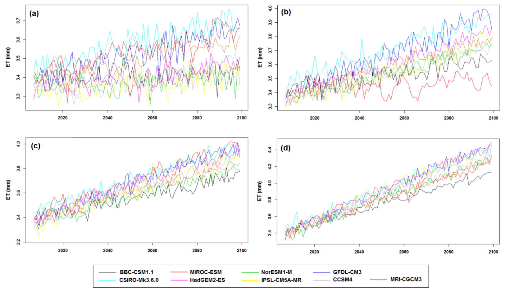
5.3. Projection of ET
6. Discussion
7. Conclusions
Author Contributions
Funding
Institutional Review Board Statement
Informed Consent Statement
Data Availability Statement
Acknowledgments
Conflicts of Interest
References
- Hamed, M.M.; Khan, N.; Shahid, S.; Muhammad, M.K.I. Ranking of Empirical Evapotranspiration Models in Different Climate Zones of Pakistan. Res. Sq. 2022. [Google Scholar] [CrossRef]
- Salehie, O.; Hamed, M.M.; Ismail, T.B.; Shahid, S. Projection of droughts in Amu river basin for shared socioeconomic pathways CMIP6. Theor. Appl. Climatol. 2022, 149, 1009–1027. [Google Scholar] [CrossRef]
- Kumar, R.; Jat, M.K.; Shankar, V. Methods to estimate irrigated reference crop evapotranspiration–a review. Water Sci. Technol. 2012, 66, 525–535. [Google Scholar] [CrossRef]
- Wigmosta, M.S.; Vail, L.W.; Lettenmaier, D.P. A distributed hydrology-vegetation model for complex terrain. Water Resour. Res. 1994, 30, 1665–1679. [Google Scholar] [CrossRef]
- Jhajharia, D.; Kumar, R.; Dabral, P.P.; Singh, V.P.; Choudhary, R.R.; Dinpashoh, Y. Reference evapotranspiration under changing climate over the Thar Desert in India. Meteorol. Appl. 2015, 22, 425–435. [Google Scholar] [CrossRef]
- Ashfaq, M.; Bowling, L.C.; Cherkauer, K. Influence of climate model biases and daily-scale temperature and precipitation events on hydrological impacts assessment: A case study of the United States. J. Geophys. Res. 2010, 115, D14116. [Google Scholar] [CrossRef]
- Kumar, R.; Kumar, M. Evaluation of reference evapotranspiration models using single crop coefficient method and lysimeter data. Indian J. Agric. Sci. 2017, 87, 350–354. [Google Scholar]
- Shiru, M.S.; Chung, E.-S.; Shahid, S. Empirical Model for the Assessment of Climate Change Impacts on Spatial Pattern of Water Availability in Nigeria BT-Intelligent Data Analytics for Decision-Support Systems in Hazard Mitigation: Theory and Practice of Hazard Mitigation; Deo, R.C., Samui, P., Kisi, O., Yaseen, Z.M., Eds.; Springer: Singapore, 2021; pp. 405–427. ISBN 978-981-15-5772-9. [Google Scholar]
- Adnan, R.M.; Heddam, S.; Yaseen, Z.M.; Shahid, S.; Kisi, O.; Li, B. Prediction of Potential Evapotranspiration Using Temperature-Based Heuristic Approaches. Sustainability 2021, 13, 297. [Google Scholar] [CrossRef]
- Jerin, J.N.; Islam, H.M.T.; Islam, A.R.M.T.; Shahid, S.; Hu, Z.; Badhan, M.A.; Chu, R.; Elbeltagi, A. Spatiotemporal trends in reference evapotranspiration and its driving factors in Bangladesh. Theor. Appl. Climatol. 2021, 144, 793–808. [Google Scholar] [CrossRef]
- Vishwakarma, D.K.; Pandey, K.; Kaur, A.; Kushwaha, N.L.; Kumar, R.; Ali, R.; Elbeltagi, A.; Kuriqi, A. Methods to estimate evapotranspiration in humid and subtropical climate conditions. Agric. Water Manag. 2022, 261, 107378. [Google Scholar] [CrossRef]
- Hamed, M.M.; Salem, M.; Shamsuddin, N.; Tarmizi, S. Thermal bioclimatic indicators over Southeast Asia: Present status and future projection using CMIP6. Environ. Sci. Pollut. Res. 2022, 1–20. [Google Scholar] [CrossRef] [PubMed]
- Alamgir, M.; Shahid, S.; Hazarika, M.K.; Nashrrullah, S.; Harun, S.B.; Shamsudin, S. Analysis of Meteorological Drought Pattern During Different Climatic and Cropping Seasons in Bangladesh. JAWRA J. Am. Water Resour. Assoc. 2015, 51, 794–806. [Google Scholar] [CrossRef]
- Salehie, O.; Ismail, T.B.; Hamed, M.M.; Shahid, S.; Idlan Muhammad, M.K. Projection of Hot and Cold Extremes in the Amu River Basin of Central Asia using GCMs CMIP6. Stoch. Environ. Res. Risk Assess. 2022, 1–22. [Google Scholar] [CrossRef]
- Bashir, T.; Kumar, R. Simulation of Modeling of Water Ecohydrologic Dynamics in a Multilayer Root Zone under Protected Conditions in the Temperate Region of India. J. Hydrol. Eng. 2017, 22, 5017020. [Google Scholar] [CrossRef]
- Muhammad, M.K.I.; Nashwan, M.S.; Shahid, S.; Ismail, T.B.; Song, Y.H.; Chung, E.S. Evaluation of empirical reference evapotranspiration models using compromise programming: A case study of Peninsular Malaysia. Sustainability 2019, 11, 4267. [Google Scholar] [CrossRef]
- Tukimat, N.N.A.N.A.; Harun, S.; Shahid, S. Comparison of different methods in estimating potential évapotranspiration at Muda Irrigation Scheme of Malaysia. J. Agric. Rural Dev. Trop. Subtrop. 2012, 113, 77–85. [Google Scholar]
- Pour, S.H.; Wahab, A.K.A.; Shahid, S.; Ismail, Z. Bin Changes in reference evapotranspiration and its driving factors in peninsular Malaysia. Atmos. Res. 2020, 246, 105096. [Google Scholar] [CrossRef]
- Muhammad, M.K.I.; Shahid, S.; Ismail, T.; Harun, S.; Kisi, O.; Yaseen, Z.M. The development of evolutionary computing model for simulating reference evapotranspiration over Peninsular Malaysia. Theor. Appl. Climatol. 2021, 144, 1419–1434. [Google Scholar] [CrossRef]
- Courault, D.; Seguin, B.; Olioso, A. Review on estimation of evapotranspiration from remote sensing data: From empirical to numerical modeling approaches. Irrig. Drain. Syst. 2005, 19, 223–249. [Google Scholar] [CrossRef]
- Liou, Y.A.; Kar, S.K. Evapotranspiration estimation with remote sensing and various surface energy balance algorithms-a review. Energies 2014, 7, 2821–2849. [Google Scholar] [CrossRef]
- Zhang, K.; Kimball, J.S.; Running, S.W. A review of remote sensing based actual evapotranspiration estimation. WIREs Water 2016, 3, 834–853. [Google Scholar] [CrossRef]
- Zhan, X.; Fang, L.; Yin, J.; Schull, M.; Liu, J.; Hain, C.; Anderson, M.; Kustas, W.; Kalluri, S. Remote Sensing of Evapotranspiration for Global Drought Monitoring. Glob. Drought Flood 2021, 29–46. [Google Scholar] [CrossRef]
- Ahmadi, F.; Nazeri Tahroudi, M.; Mirabbasi, R.; Kumar, R. Spatiotemporal analysis of precipitation and temperature concentration using PCI and TCI: A case study of Khuzestan Province, Iran. Theor. Appl. Climatol. 2022, 149, 743–760. [Google Scholar] [CrossRef]
- Sobh, M.T.; Nashwan, M.S.; Amer, N. High Resolution Reference Evapotranspiration for Arid Egypt: Comparative analysis and evaluation of empirical and artificial intelligence models. Res. Sq. 2022. [Google Scholar] [CrossRef]
- Ye, L.; Zahra, M.M.A.; Al-Bedyry, N.K.; Yaseen, Z.M. Daily scale evapotranspiration prediction over the coastal region of southwest Bangladesh: New development of artificial intelligence model. Stoch. Environ. Res. Risk Assess. 2021, 36, 451–471. [Google Scholar] [CrossRef]
- Nandagiri, L.; Kovoor, G.M. Performance Evaluation of Reference Evapotranspiration Equations across a Range of Indian Climates. J. Irrig. Drain. Eng. 2006, 132, 238–249. [Google Scholar] [CrossRef]
- Wei, G.; Zhang, X.; Ye, M.; Yue, N.; Kan, F. Bayesian performance evaluation of evapotranspiration models based on eddy covariance systems in an arid region. Hydrol. Earth Syst. Sci. 2019, 23, 2877–2895. [Google Scholar] [CrossRef]
- Penman, H.L. Natural evaporation from open water, bare soil and grass. In Proceedings of the Royal Society of London; The Royal Society London: London, UK, 1948; Volume 193, pp. 120–145. [Google Scholar]
- Salman, S.A.; Hamed, M.M.; Shahid, S.; Ahmed, K.; Sharafati, A.; Asaduzzaman, M.; Ziarh, G.F.; Ismail, T.; Chung, E.-S.; Wang, X.-J.; et al. Projecting spatiotemporal changes of precipitation and temperature in Iraq for different shared socioeconomic pathways with selected Coupled Model Intercomparison Project Phase 6. Int. J. Climatol. 2022, 1–19. [Google Scholar] [CrossRef]
- Hamed, M.M.; Nashwan, M.S.; Shahid, S.; Ismail, T.B.; Wang, X.J.; Dewan, A.; Asaduzzaman, M. Inconsistency in historical simulations and future projections of temperature and rainfall: A comparison of CMIP5 and CMIP6 models over Southeast Asia. Atmos. Res. 2022, 265, 105927. [Google Scholar] [CrossRef]
- Hamed, M.M.; Nashwan, M.S.; Shahid, S. A novel selection method of CMIP6 GCMs for robust climate projection. Int. J. Climatol. 2022, 42, 4258–4272. [Google Scholar] [CrossRef]
- Hamed, M.M.; Nashwan, M.S.; Shahid, S. Inter-comparison of Historical Simulation and Future Projection of Rainfall and Temperature by CMIP5 and CMIP6 GCMs Over Egypt. Int. J. Climatol. 2022, 42, 4316–4332. [Google Scholar] [CrossRef]
- Salehie, O.; Hamed, M.M.; Ismail, T.; Tam, T.H.; Shahid, S. Selection of CMIP6 GCM with Projection of Climate Over The Amu Darya River Basin. Res. Sq. 2021, 1–27. [Google Scholar] [CrossRef]
- Pour, S.H.; Wahab, A.K.A.; Shahid, S. Physical-empirical models for prediction of seasonal rainfall extremes of Peninsular Malaysia. Atmos. Res. 2020, 233, 104720. [Google Scholar] [CrossRef]
- Jing, W.; Yaseen, Z.M.; Shahid, S.; Saggi, M.K.; Tao, H.; Kisi, O.; Salih, S.Q.; Al-Ansari, N.; Chau, K.-W. Implementation of evolutionary computing models for reference evapotranspiration modeling: Short review, assessment and possible future research directions. Eng. Appl. Comput. fluid Mech. 2019, 13, 811–823. [Google Scholar] [CrossRef]
- Pan, S.; Pan, N.; Tian, H.; Friedlingstein, P.; Sitch, S.; Shi, H.; Arora, V.K.; Haverd, V.; Jain, A.K.; Kato, E.; et al. Evaluation of global terrestrial evapotranspiration using state-of-the-art approaches in remote sensing, machine learning and land surface modeling. Hydrol. Earth Syst. Sci. 2020, 24, 1485–1509. [Google Scholar] [CrossRef]
- Carter, C.; Liang, S. Evaluation of ten machine learning methods for estimating terrestrial evapotranspiration from remote sensing. Int. J. Appl. Earth Obs. Geoinf. 2019, 78, 86–92. [Google Scholar] [CrossRef]
- Dou, X.; Yang, Y. Evapotranspiration estimation using four different machine learning approaches in different terrestrial ecosystems. Comput. Electron. Agric. 2018, 148, 95–106. [Google Scholar] [CrossRef]
- Granata, F. Evapotranspiration evaluation models based on machine learning algorithms—A comparative study. Agric. Water Manag. 2019, 217, 303–315. [Google Scholar] [CrossRef]
- Kiafar, H.; Babazadeh, H.; Marti, P.; Kisi, O.; Landeras, G.; Karimi, S.; Shiri, J. Evaluating the generalizability of GEP models for estimating reference evapotranspiration in distant humid and arid locations. Theor. Appl. Climatol. 2017, 130, 377–389. [Google Scholar] [CrossRef]
- Mehdizadeh, S.; Behmanesh, J.; Khalili, K. Using MARS, SVM, GEP and empirical equations for estimation of monthly mean reference evapotranspiration. Comput. Electron. Agric. 2017, 139, 103–114. [Google Scholar] [CrossRef]
- Estrada-Flores, S.; Merts, I.; De Ketelaere, B.; Lammertyn, J. Development and validation of “grey-box” models for refrigeration applications: A review of key concepts. Int. J. Refrig. 2006, 29, 931–946. [Google Scholar] [CrossRef]
- Kazemi, M.H.; Majnooni-Heris, A.; Kisi, O.; Shiri, J. Generalized gene expression programming models for estimating reference evapotranspiration through cross-station assessment and exogenous data supply. Environ. Sci. Pollut. Res. 2021, 28, 6520–6532. [Google Scholar] [CrossRef] [PubMed]
- Barzkar, A.; Shahabi, S.; Niazmradi, S.; Madadi, M.R. A comparative study of remote sensing and gene expression programming for estimation of evapotranspiration in four distinctive climates. Stoch. Environ. Res. Risk Assess. 2021, 35, 1437–1452. [Google Scholar] [CrossRef]
- Tangang, F.T. Low frequency and quasi-biennial oscillations in the Malaysian precipitation anomaly. Int. J. Climatol. 2001, 21, 1199–1210. [Google Scholar] [CrossRef]
- Pour, S.H.; Shahid, S.; Chung, E.S.; Wang, X.J. Model output statistics downscaling using support vector machine for the projection of spatial and temporal changes in rainfall of Bangladesh. Atmos. Res. 2018, 213, 149–162. [Google Scholar] [CrossRef]
- Hamed, M.M.; Nashwan, M.S.; Shahid, S. Performance Evaluation of Reanalysis Precipitation Products in Egypt using Fuzzy Entropy Time Series Similarity Analysis. Int. J. Climatol. 2021, 41, 5431–5446. [Google Scholar] [CrossRef]
- Nait Amar, M. Prediction of hydrate formation temperature using gene expression programming. J. Nat. Gas. Sci. Eng. 2021, 89, 103879. [Google Scholar] [CrossRef]
- Chu, H.-H.; Khan, M.A.; Javed, M.; Zafar, A.; Ijaz Khan, M.; Alabduljabbar, H.; Qayyum, S. Sustainable use of fly-ash: Use of gene-expression programming (GEP) and multi-expression programming (MEP) for forecasting the compressive strength geopolymer concrete. Ain Shams Eng. J. 2021, 12, 3603–3617. [Google Scholar] [CrossRef]
- Kotanchek, M.E.; Vladislavleva, E.Y.; Smits, G.F. Symbolic Regression Via Genetic Programming as a Discovery Engine: Insights on Outliers and Prototypes BT-Genetic Programming Theory and Practice VII; Riolo, R., O’Reilly, U.-M., McConaghy, T., Eds.; Springer: Boston, MA, USA, 2010; pp. 55–72. ISBN 978-1-4419-1626-6. [Google Scholar]
- Koza, J.R. Evolution of subsumption using genetic programming. In Proceedings of the First European Conference on Artificial Life; MIT Press: Cambridge, MA, USA, 1992; pp. 110–119. [Google Scholar]
- Doorenbos, J.; Pruitt, W.O. Crop water requirements. FAO Irrigation and Drainage Paper 24. In Land and Water Development Division; FAO: Rome, Italy, 1977; Volume 144. [Google Scholar]
- Linacre, E.T. A simple formula for estimating evaporation rates in various climates, using temperature data alone. Agric. Meteorol. 1977, 18, 409–424. [Google Scholar] [CrossRef]
- Kharrufa, N.S. Simplified equation for evapotranspiration in arid regions. Beiträge Hydrol. 1985, 5, 39–47. [Google Scholar]
- Hargreaves, G.; Samani, Z. Reference Crop Evapotranspiration from Temperature. Appl. Eng. Agric. 1985, 1, 96–99. [Google Scholar] [CrossRef]
- Trajkovic, S. Hargreaves versus Penman-Monteith under Humid Conditions. J. Irrig. Drain. Eng. 2007, 133, 38–42. [Google Scholar] [CrossRef]
- Ravazzani, G.; Corbari, C.; Morella, S.; Gianoli, P.; Mancini, M. Modified Hargreaves-Samani Equation for the Assessment of Reference Evapotranspiration in Alpine River Basins. J. Irrig. Drain. Eng. 2012, 138, 592–599. [Google Scholar] [CrossRef]
- Taylor, K.E.; Stouffer, R.J.; Meehl, G.A. An overview of CMIP5 and the experiment design. Bull. Am. Meteorol. Soc. 2012, 93, 485–498. [Google Scholar] [CrossRef]
- Van Vuuren, D.P.; Edmonds, J.; Kainuma, M.; Riahi, K.; Thomson, A.; Hibbard, K.; Hurtt, G.C.; Kram, T.; Krey, V.; Lamarque, J.F.; et al. The representative concentration pathways: An overview. Clim. Chang. 2011, 109, 5–31. [Google Scholar] [CrossRef]
- IPCC. Climate Change 2013: The Physical Science Basis; IPCC: Cambridge, UK; New York, NY, USA, 2013. [Google Scholar]


| Model Developing Institute | Model Name | Resolution (Lon × Lat) |
|---|---|---|
| Beijing Climate Center, China | BCC-CSM1.1 | 2.8° × 2.8° |
| National Center for Atmospheric Research, USA | CCSM4 | 1.25° × 0.94° |
| Met Office Hadley Centre, UK | HadGEM2-ES | 1.87° × 1.25° |
| Atmosphere and Ocean Research Institute, The University of Tokyo, Japan | MIROC-ESM | 2.8° × 2.8° |
| Bjerknes Centre for Climate Research, Norwegian Meteorological Institute, Norway | NorESM1-M | 2.5° × 1.9° |
| Geophysical Fluid Dynamics Laboratory, USA | GFDL-CM3 | 2.5° × 2.0° |
| Commonwealth Scientific and Industrial Research Organization, Australia | CSIRO-Mk3.6.0 | 1.86° × 1.87° |
| Institut Pierre Simon Laplace, France | IPSL-CM5A-MR | 1.26° × 2.5° |
| Meteorological Research Institute, Japan | MRI-CGCM3 | 1.12° × 1.12° |
| No | Model | Input Parameter | Equation |
|---|---|---|---|
| 1 | FAO Blaney-Criddle [53] | Tmean | |
| 2 | Linacre [54] | Tmean | |
| 3 | Kharrufa [55] | Tmean | |
| 4 | Hargreaves and Samani [56] | Tmean, Tmin, Tmax, Ra | |
| 5 | Trajkovic [57] | Tmean, Tmin, Tmax, Ra | |
| 6 | Ravazzani [58] | Tmean, Tmin, Tmax, Ra |
| Station Name | Model |
|---|---|
| Alor Setar | [(0.708527 + Tmax + (Tmax/−0.570404)) × ((Tmax + Tmin) × (0.708527/Tmax))] + [0.271 × Tmin−4.310577] + [Tmax−((39.983448 + Tmin)/(6.337066 + Tmin))] |
| Bayan Lepas | [−2.659455/(Tmin + ((Tmin + Tmax) × (−2.659455/Tmax)))] − [9.144561] + [((Tmax + 2.659455) × Tmax)/(Tmin + 1.002563 + 2 × Tmax)] |
| Ipoh | [−9.89798−Tmin] + [(2 × Tmax−Tmin + 2.245544)/8.36405] + [Tmin + 7.706391] |
| Kota Bharu | ((Tmax/4.688568) − (4.688568/Tmin) − 4.688568) + (−1.946625/((Tmin× −1.946625) + Tmax + 5.589417)) + (Tmax/(Tmin − ((Tmin + Tmax)/(Tmin^2)))) |
| Kuala Terenggannu | (Tmax/5.405304) + ((2 × Tmax + 2 × Tmin)/((Tmax^0.13211) + (Tmax × 5.950409)))+ ((Tmin + Tmax)/(12.843872 − Tmax)) |
| Kuantan | (((Tmin × −1.63205) + (Tmin/−1.63205))/((Tmin × Tmax)/(Tmin − 1.63205))) + (((−4.044677/(Tmin/Tmax)) + 1.682221 − Tmax)/−4.044677) − 4.384247 |
| Melaka | ((−8.459076 + Tmax)/Tmax) + ((Tmax − Tmin)/((2 × Tmax)/(0.269501 + Tmax))) + (−8.391388/(Tmin − 18.419738)) |
| Muadzam Shah | [((Tmin − Tmax)/(7.168945 − Tmax))/((7.168945/Tmax) − 7.411835)] + [((−6.097015/Tmin) − (4.724793 + Tmin))/((Tmax × 4.724793) + (−6.097015/Tmax))] + [((Tmin − Tmax)/(−9.070129 − Tmax))/(1.893555/Tmin)] |
| Senai | [(−5.88443 − Tmin + Tmax)/(−3.50461 + 2Tmin)] + [−10.39233/(Tmin − 14.90024)] + [2Tmax2/Tmin2] |
| Subang | [−4.079162/Tmin] + [(6.476776 − Tmin)/(Tmax/(Tmin − Tmax))] + [−14.214936/(−12.751648 + Tmin)] |
| Station Name | NSE | MAE | RMSE | md |
|---|---|---|---|---|
| Alor Setar | 0.98 | 4.7 | 7.9 | 1.0 |
| Senai | 0.94 | 5.4 | 7.6 | 0.9 |
| Bayan Lepas | 0.92 | 6.6 | 8.9 | 0.9 |
| Ipoh | 0.81 | 7.3 | 9.3 | 0.7 |
| Muadzam Shah | 0.79 | 6.9 | 8.9 | 0.8 |
| Subang | 0.76 | 6.1 | 7.6 | 0.7 |
| Kuantan | 0.99 | 3.3 | 4.8 | 1.0 |
| Melaka | 0.94 | 6.1 | 9.3 | 0.9 |
| Kota Bharu | 0.87 | 10.1 | 12.1 | 0.8 |
| Kuala Terenggannu | 0.95 | 5.8 | 10.3 | 0.9 |
Publisher’s Note: MDPI stays neutral with regard to jurisdictional claims in published maps and institutional affiliations. |
© 2022 by the authors. Licensee MDPI, Basel, Switzerland. This article is an open access article distributed under the terms and conditions of the Creative Commons Attribution (CC BY) license (https://creativecommons.org/licenses/by/4.0/).
Share and Cite
Muhammad, M.K.I.; Shahid, S.; Hamed, M.M.; Harun, S.; Ismail, T.; Wang, X. Development of a Temperature-Based Model Using Machine Learning Algorithms for the Projection of Evapotranspiration of Peninsular Malaysia. Water 2022, 14, 2858. https://doi.org/10.3390/w14182858
Muhammad MKI, Shahid S, Hamed MM, Harun S, Ismail T, Wang X. Development of a Temperature-Based Model Using Machine Learning Algorithms for the Projection of Evapotranspiration of Peninsular Malaysia. Water. 2022; 14(18):2858. https://doi.org/10.3390/w14182858
Chicago/Turabian StyleMuhammad, Mohd Khairul Idlan, Shamsuddin Shahid, Mohammed Magdy Hamed, Sobri Harun, Tarmizi Ismail, and Xiaojun Wang. 2022. "Development of a Temperature-Based Model Using Machine Learning Algorithms for the Projection of Evapotranspiration of Peninsular Malaysia" Water 14, no. 18: 2858. https://doi.org/10.3390/w14182858