Hydrological Response to Meteorological Droughts in the Guadalquivir River Basin, Southern Iberian Peninsula

Abstract

Drought is an extreme phenomenon that will likely increase in frequency and severity in the current context of climate change. As such, it must be studied to improve the decision-making process in affected areas. As a semi-arid zone, the Guadalquivir River basin, located in the southern Iberian Peninsula, is an interesting area to perform this study. The relationship between meteorological and hydrological droughts is studied using drought indices with data from 1980 to 2012. The chosen indices are the Standardized Streamflow Index (SSI) and the Standardized Precipitation Evapotranspiration Index (SPEI). Their correlations are calculated, based on SPEI accumulation periods, and these values are analyzed with a principal component analysis to find spatial patterns in drought behavior inside the basin. This analysis was performed for the continuous series and also for monthly series, to account for seasonal changes. It has been found that the relationship of drought types occurs at different time scales depending mainly on orography and catchment area. Two main patterns were found. Generally, for low altitudes and small catchment areas, accumulation periods are shorter indicating that hydrological system in this area respond rapidly to meteorological conditions. In mountainous parts of the basin, longer accumulation periods have a stronger influence due to effects such as snowmelt.

1. Introduction

Several regions around the world, their populations, and their economies, are currently affected by the extreme phenomenon of drought [1]. Climate change projections using regional models show that some arid and semiarid areas, such as the Iberian Peninsula, will likely suffer an increase in the number and severity of droughts [2,3]. Therefore, such extreme events must be studied in order to understand their mechanisms and how different parameters affect their development.

One of the mechanisms that can be studied is the relationship between different drought types. The definition of drought type depends on the variable that determines the occurrence of drought. For example, meteorological drought happens when rainfall is lower than a certain threshold; in contrast, hydrological drought appears when streamflow and runoff are lower than normal. Depending on the purpose of the definition, the timeframe may span from weeks or months used in policies to years used in megadrought studies. The relationship between hydrological and meteorological droughts has been studied in different areas of the world [4,5,6,7,8], and it depends on factors such as climate characteristics and orography [9,10]. Therefore, it is not an immediate conclusion that hydrological drought will happen shortly after meteorological drought. On the contrary, it requires a detailed quantitative analysis on each basin.

Drought indices are one of the tools that can be used to perform the aforementioned quantitative analyses. There are a plethora of indices, and each of them has a different application. To define meteorological droughts, the classic Standardized Precipitation Index, SPI [11], considers only precipitation in order to assess the occurrence of droughts or wet periods in an area, but several other indices have been developed after SPI. Each of those indices takes into account the different climate parameters. In this study, two indices are used: the Standardized Precipitation Evapotranspiration Index, SPEI [12], and the Standardized Streamflow Index, SSI [13]. SPEI describes meteorological drought through the use of precipitation and potential evapotranspiration data. By choosing SPEI over SPI, the role of temperature increase is better accounted for when evaluating drought conditions, particularly during periods of precipitation deficits over water-limited regions [14], which is important in the current context of climate change [15,16]. Meanwhile, SSI describes hydrological drought through the use of streamflow data. One of the advantages of SSI over other hydrological indices is that it chooses between six probability distributions to adjust streamflow data. Since hydrological processes are highly dependent on the orography, not having a fixed probability distribution allows for a better, more flexible characterization of the spatial particularities of the basin. At the same time, it has the benefit of all standardized indices in that they allow for robust drought comparisons between different spatial points [13]. Other hydrological drought indices, such as the Regional Deficiency Index, only describe duration and severity of droughts, not magnitude [17]. Additionally, spatial comparisons are not as reliable as with standardized indices such as SSI [17].

The Guadalquivir River basin is a semi-arid area located in the South of the Iberian Peninsula. Its main river, the Guadalquivir, is the fifth longest river in the Iberian Peninsula with 657 km. Yearly water demands in this area are around 3568 hm³, while yearly availability ranges from 372 hm³ to 21,530 hm³ [18]. As water deficits are likely to increase due to climate change, it is of upmost importance to understand how hydrological and meteorological droughts influence each other in the basin. Understanding the relationship between both drought types, also called drought propagation [19], will be beneficial to manage water resources in the area [20], which is likely to become a critical task in the near future. This topic is currently being studied in different areas using other indices [21,22,23], and it is also interesting for evaluating changes in groundwater resources [24]. Additionally, the potential impact of reservoirs in the relationship of both drought types has been explored [25], and will be discussed later in this paper since several regulation infrastructures have been built in the studied basin in the past. While there are methodologies that focus on the dry periods of the drought indices, studying duration, severity, and magnitude of drought events, such methodologies are not adequate to consider the evolution of human-induced hydrological changes [26]. Therefore, they are not used in this analysis.

The main objective of this work is to study the hydrological response to meteorological droughts in the Guadalquivir basin, taking into account the existing regulation infrastructures. This aim is completed by classifying the basin into different sub-areas which show similar correlation patterns between SPEI and SSI, i.e., between meteorological and hydrological droughts.

Section 2 explains the data used, including a description of the study area, and the methodological approach. Section 3 explains the main findings of the study. Lastly, the conclusions in Section 4 sum up the results and explain how they can be further used in future studies.

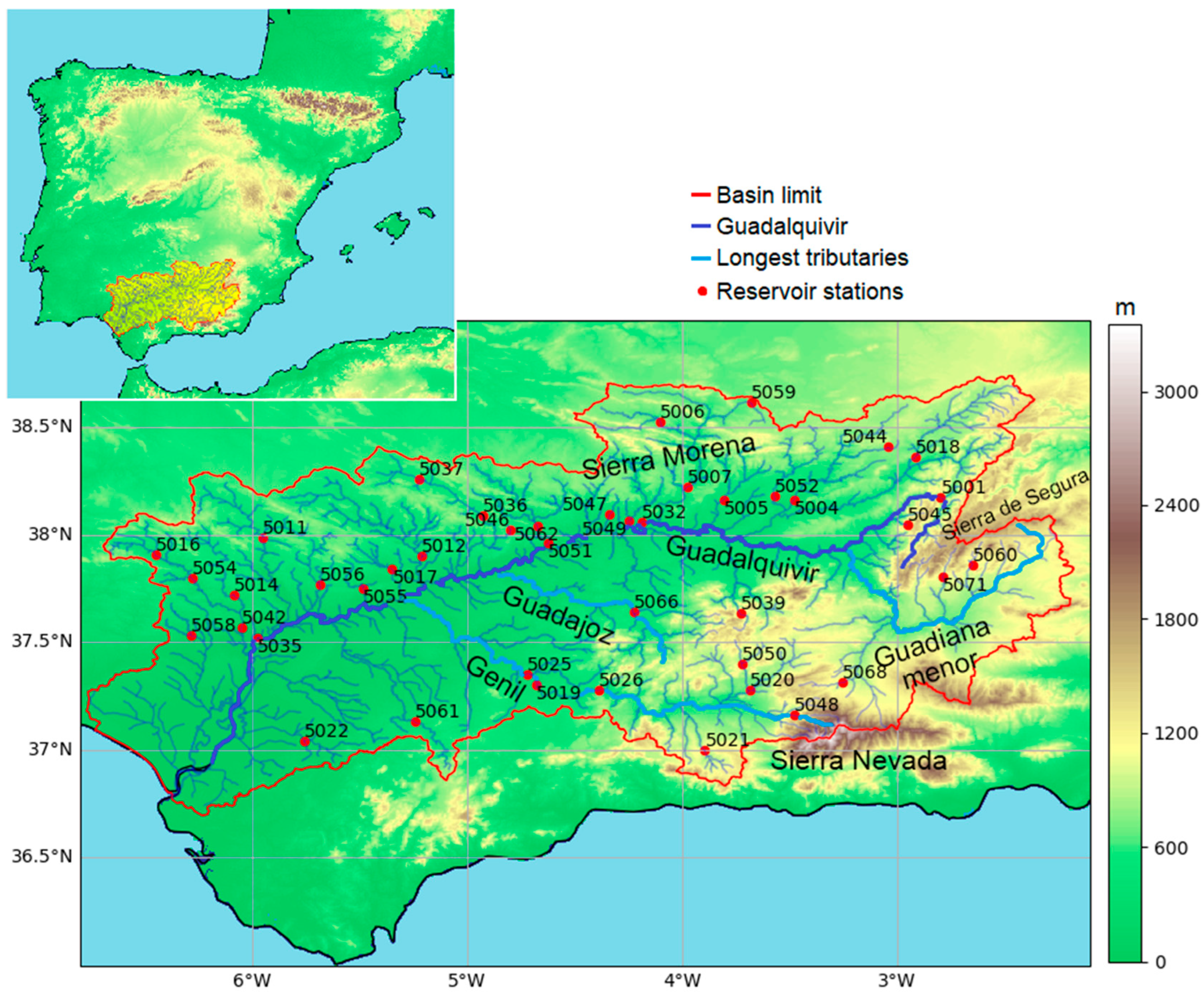
2. Data and Methodology

The study area is located in the south of the Iberian Peninsula. Figure 1 depicts the main features of its orography. Guadalquivir River has several tributaries, which can at first glance be divided into two groups: the ones to the south of Guadalquivir, which are longer, and the ones to the north, which are shorter. The presence of small rivers in this dry area, together with the necessity to avoid water deficit, has historically led to the construction of several dams and reservoirs to supply for agricultural and human water needs in the area. Therefore, there is a high regulation in streamflow, which makes it an interesting area to study. For example, precipitation in the summer months (particularly in July and August) is almost zero in several parts of the basin, but reservoirs must supply a minimum ecological streamflow. Therefore, the correlation between precipitation and streamflow is cancelled because of human activities. During higher-precipitation months, normally from November to February, with December reaching more than 3000 mm in extreme cases, or when extreme flood events occur, the streamflow released from dams is higher, so the correlation should increase.

Regarding the orography, the Guadalquivir basin consists of mountainous areas to the north and southeast, with a high presence of limestone and conglomerate. The northern mountain range, Sierra Morena, is composed of low permeability soils, while soils in the southeastern mountains of Sierra Nevada and Sierra de Segura show moderate permeability [18]. A long valley is located in the center of the basin, crossing from east to west, where the Guadalquivir flows. The river ends in a marsh area in the southwest of the basin. As can be inferred from this description, the area cannot be defined as homogeneous, increasing its interest as the place to study the relationship between drought types. Concerning the relationship between precipitation and streamflow, during spring months (from March to May), streamflow will increase due to snowmelt, that is, due to precipitation from past months. Therefore, different precipitation regimes can be found in this basin: rainfall regime, snowmelt and rainfall regime, and human-induced regime due to regulation [27].

This study used high quality observational data for the variables required in the calculation of drought indices: precipitation, potential evapotranspiration, and streamflow. Precipitation was obtained from the Spanish Precipitation at Daily Scale (SPREAD) dataset [28]. This dataset comprises gridded data based on previous observations. One of the reasons to choose this dataset is that the dimension of grid squares is 5 km, which is enough to describe precipitation in the entirety of the Guadalquivir basin at a fine and appropriate resolution. Potential evapotranspiration was extracted from the Spanish Reference Evapotranspiration (SPETo) gridded database [29]. This dataset contains weekly data at a resolution of 1.1 km, and it has been calculated using temperature, wind speed, dewpoint temperature, and sunshine duration data by using the Penman-Monteith formulation [30]. Regarding streamflow data, the main source of observational data is the Guadalquivir hydrographic authority (Confederación Hidrográfica del Guadalquivir) website [31], where data are freely available. Particularly, monthly reservoir data have a high quality with respect to series duration and low presence of gaps and inconsistencies. Nevertheless, some stations still showed gaps or had a short data timespan. These stations were not included in the analysis. Furthermore, time series had to be trimmed so that their data were simultaneous. SPREAD and SPETo end in December 2012, while most streamflow data begin or improve their quality in January 1980. Therefore, the shared dates of the three databases range from January 1980 to December 2012, and this is the period of study.

When managing streamflow data from reservoirs, there are two main values to consider: inflow and outflow. Inflow depends on the physical characteristics of the catchment basin, while outflow is totally dependent on dam operation. Certainly, the outflow is higher when extreme precipitation events occur, since dam sluices are opened to avoid floods. It is, however, more interesting for this study to consider only inflow data. The reason is the important human interaction component present in outflow data, which distorts the correlation between precipitation and streamflow. Therefore, for the purpose of this work, only inflow has been used to calculate the aforementioned relationships. Note, however, that inflow data are also affected by regulation from upstream reservoirs. Nevertheless, the impact of such reservoirs is lowered the further they are from the data source. Considering this explanation, the reservoirs that provided no useful information because of this effect, i.e., reservoirs that had another reservoir few kilometers upstream, were excluded from the analysis.

After discarding 19 stations with insufficient data quality or quantity, data from 43 reservoir stations for the period 1980–2012 were used to perform this study. The designation of these stations, as shown in Figure 1 and

Table 1. Characteristics of reservoir stations used in this study.

Reference	Longitude [o]	Latitude [o]	Mean Monthly Streamflow (m3/s)	Altitude [m]	Area [km2]	Permeability [%]
5001	−2.795	38.175	13.08	550	550	78.13
5004	−3.476	38.164	11.07	296	1330	1.07
5005	−3.804	38.161	7.18	276	550	0
5006	−4.099	38.526	5.65	511	557.48	10.01
5007	−3.973	38.227	16.35	276	2300	2.31
5011	−5.952	37.985	13.57	256	1100	32.26
5012	−5.209	37.903	22.43	86.2	1078.5	23.87
5014	−6.087	37.72	10.48	228.92	525	0
5016	−6.45	37.909	7.71	286	408	4.02
5017	−5.348	37.843	6.13	136	311	85.11
5018	−2.913	38.365	11.31	506	1323	5.38
5019	−4.676	37.301	28.84	214	5219	16.73
5020	−3.681	37.277	3.39	605.4	626	55.49
5021	−3.892	36.997	3.85	769	307	24.61
5022	−5.757	37.043	6.45	13	460	18.10
5025	−4.72	37.351	31.87	173	5830	29.49
5026	−4.386	37.278	31.59	304	5000	20.13
5032	−4.185	38.06	73.65	174	20,137	36.18
5035	−5.975	37.52	186.46	8	46,860	91.94
5036	−4.924	38.088	12.60	391.5	980	0
5037	−5.222	38.26	4.34	470	439	5.24
5039	−3.727	37.635	1.17	705	99	63.44
5042	−6.049	37.569	18.67	6.5	1755	1.42
5044	−3.038	38.409	0.63	681.3	62.59	9.91
5045	−2.951	38.047	1.03	960.3	18	77.30
5046	−4.798	38.022	0.58	487.5	28	0
5047	−4.339	38.094	1.22	231	48.26	0
5048	−3.475	37.161	5.35	808	176	76.51
5049	−4.249	38.069	14.61	167.75	790	0
5050	−3.72	37.402	2.06	755	245	32.16
5051	−4.624	37.961	17.51	105	1287	1.05
5052	−3.569	38.181	9.94	356	663	0
5054	−6.279	37.798	15.76	190	850	4.49
5055	−5.484	37.749	6.01	73.65	243	28.35
5056	−5.684	37.772	11.18	207	459	9.96
5058	−6.283	37.534	6.70	63.8	228	3.82
5059	−3.68	38.618	2.27	681	135.12	0
5060	−2.647	37.859	2.09	972.5	152	38.04
5061	−5.242	37.131	3.77	207	297.6	1.72
5062	−4.673	38.043	17.47	151.5	1209	0
5066	−4.225	37.64	10.23	294	1185	3.44
5068	−3.254	37.314	1.40	870	184.4	47.24
5071	−2.786	37.807	5.70	837.5	110	51.29

, is taken from the aforementioned database of observational reservoir data. For these stations, drought indices were calculated. Geographically, the most restrictive variable was the streamflow, since it stands as a series of non-grid points. Consequently, the 43 closest grid points from SPREAD and SPETo datasets were chosen for the calculation of SPEI.

The drought indices calculation is slightly different for SPEI and SSI. When computing SPEI, the hydrological balance (i.e., the difference between precipitation and evapotranspiration) is calculated as a monthly series, adding values from previous months depending on the accumulation period, which in this study ranges from 1 to 24. These data are then adjusted to a log-logistic distribution [12] in order to compute the probability series. These values must then be normalized [32], giving as a result the values of the drought index. Regarding SSI, streamflow data cannot be accumulated when calculating index values [13], so the accumulation period concept is not relevant for SSI. Additionally, the distribution to which the data must be adjusted has to be chosen between the following six [13]: Generalized Extreme Values, Pearson type III, Log-logistic, Log-normal, Pareto, and Weibull. The best-fitting distribution needs to be chosen for each station, and after obtaining its probability values, the final index values are calculated following the same methodology of SPEI.

By correlating the 1–24 months accumulated SPEI indices with SSI, which accounts only for the current month, the propagation from meteorological to hydrological drought can be analyzed for different areas of the river basin [5,33]. This response has been analyzed in two separate ways: on the one hand, the continuous SSI and SPEI series from 1980 to 2012 have been compared; on the other hand, both series were divided into months, showing how the relationship varies in different moments of the hydrological year. Additionally, the second monthly analysis could be helpful to identify the moment when the hydrological year starts in the Guadalquivir basin, since its definition is related to the correlation between precipitation and streamflow [34].

The proposed methodology, that correlates monthly SSI with multi-scale SPEI, intends to easily evaluate the response time of hydrological drought [35] and has been successfully applied in other basins in the Iberian Peninsula [5].

After computing correlations, a principal component analysis (PCA) was performed in order to analyze the different spatial patterns of correlation between the SSI and the SPEI at different time scales. PCA is widely used in climate research to find patterns in the data from a complex dataset [36,37]. The purpose of this PCA was to check if the basin could be divided in sub-basins with similar hydrological responses. It was performed using both the continuous series and the monthly series, and the divisions were made using the PCA scores and loadings.

PCA was performed in S-mode, so that the PCA explores relationships between the time series of the grid points, as opposed to T-mode, which explores relationships for a given event. Since the aim is to study spatial patterns of stations with a similar behavior of correlations between SPEI and SSI, S-mode is used [38]. PCA is able to reduce a large number of interrelated variables to a few independent principal components (PCs) that capture much of the variance of the original dataset. Moreover, it produces a few major spatial variability patterns (or empirical orthogonal functions, EOFs). Additionally, a varimax rotation was applied to the components, thus maximizing the variance of the squared correlation coefficients, and therefore better capturing the physically meaningful and simplified spatial patterns. This procedure allows the extraction of representative stations for each of the areas obtained in the regionalization process. Consequently, by performing this transformation, the found patterns were physically more stable [39], and it was easier to understand the information given by loadings [40]. Thus, scores of a given principal component show what accumulation periods dominate the correlation of stations with high loadings for the same principal component. By describing the basin with more than one principal component, different accumulation periods can be considered in the analysis.

Finally, the last part of the analysis includes a multilinear regression that tries to find if the patterns found during the PCA can be explained by the geographical characteristics of the basin. To this end, the loading obtained for each PC and for each station is introduced together with its values for the geographical variables in a linear regression model. Then, p-values of each variable are compared to find which ones are more relevant for each PC. The geographical variables were station altitude (Figure 1), catchment area (Figure 2a), and percentage of permeable soil in that catchment area (Figure 2b). This way, it is possible to elucidate if the similarities in drought behavior (obtained by means of the PCA) can be explained by the physical characteristics of the stations. The variables corresponding to each station are detailed in Table 1.

For clarity purposes, the methodology has been represented as a flowchart in Figure 3.

3. Results and Discussion

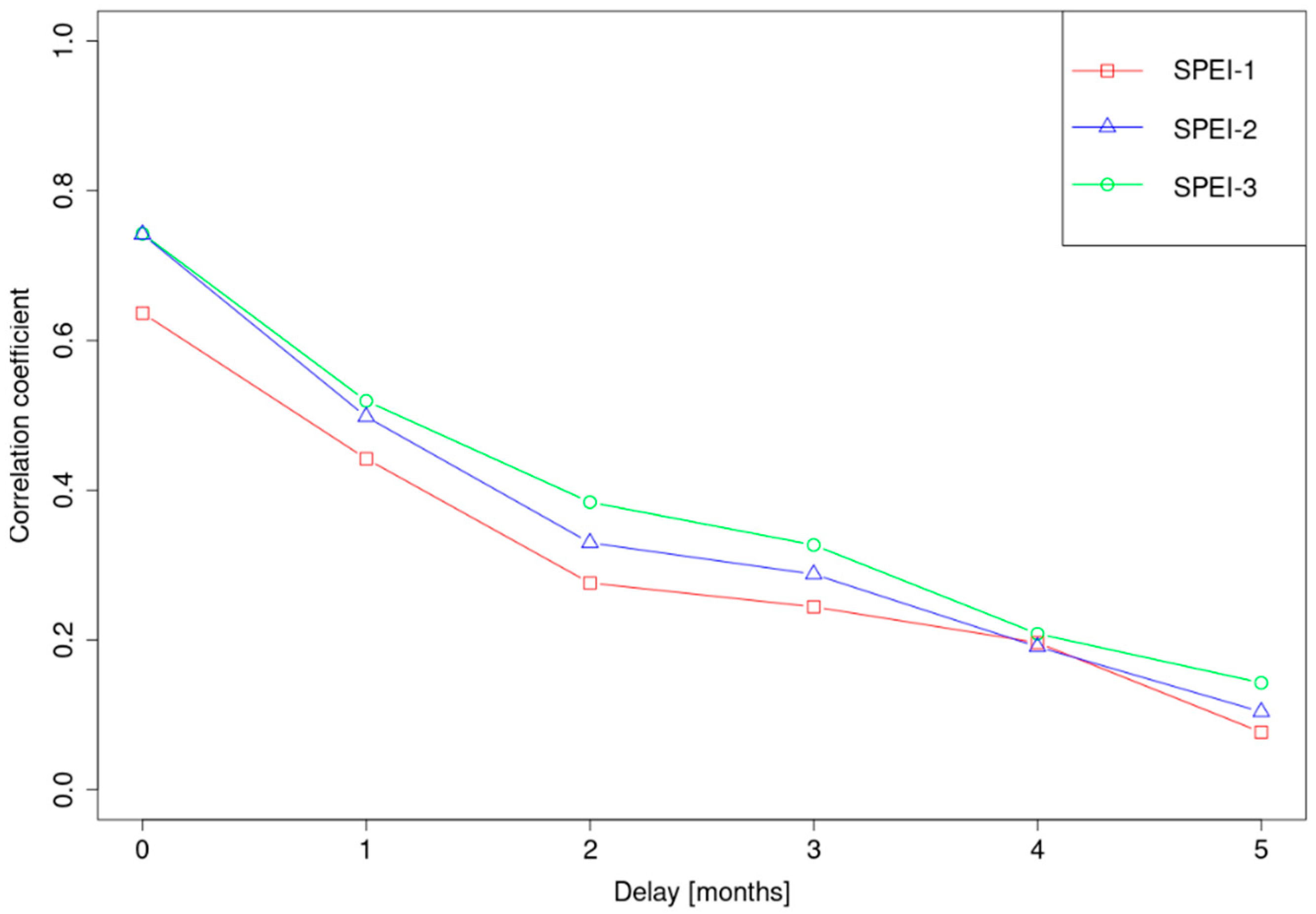
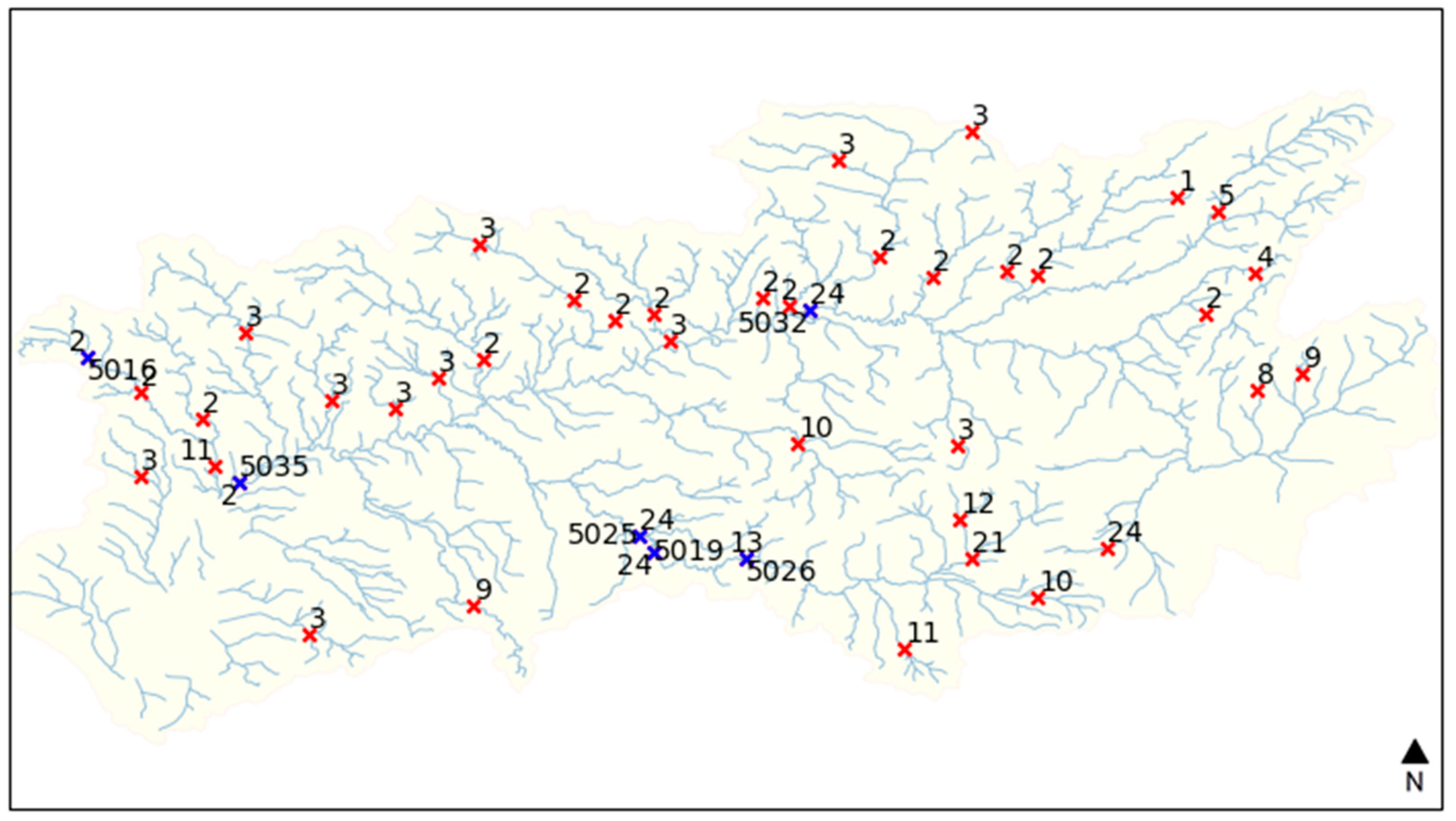
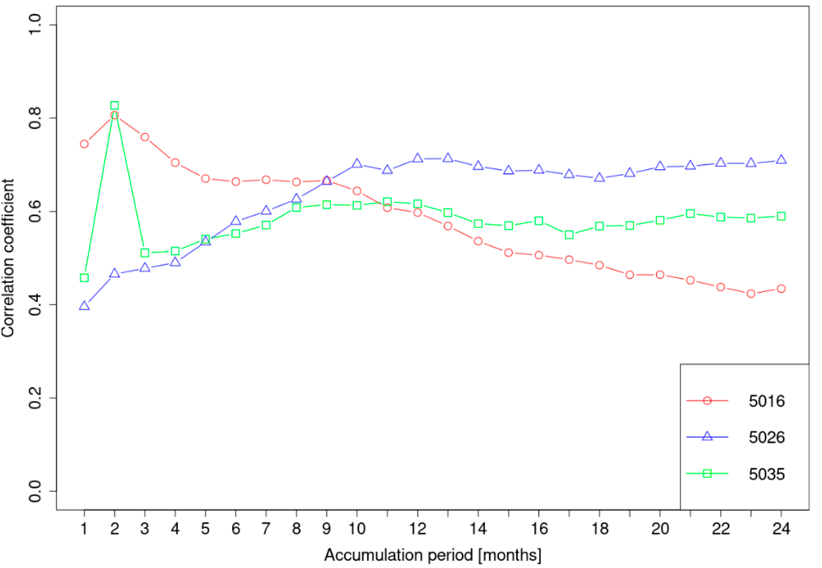
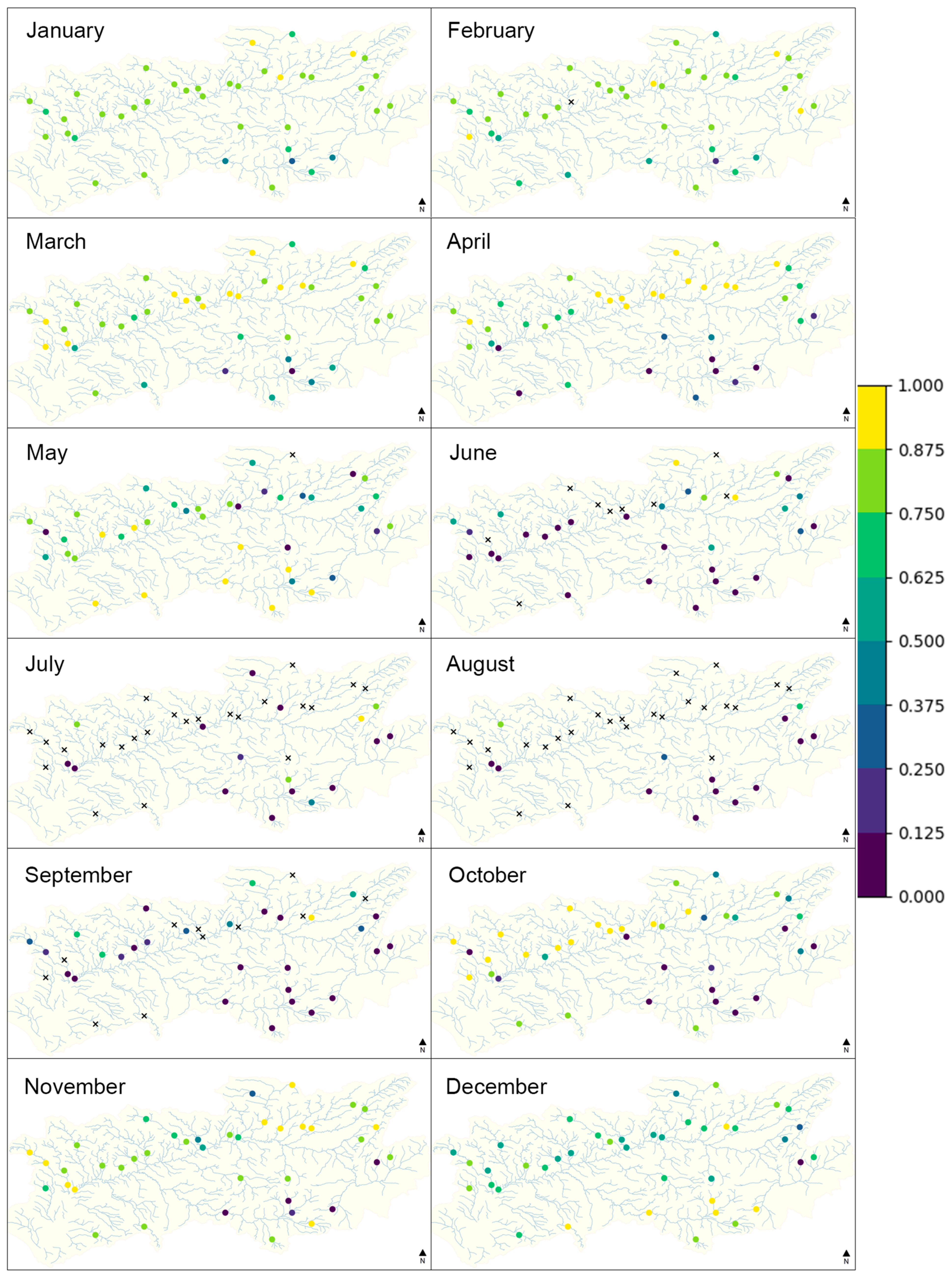
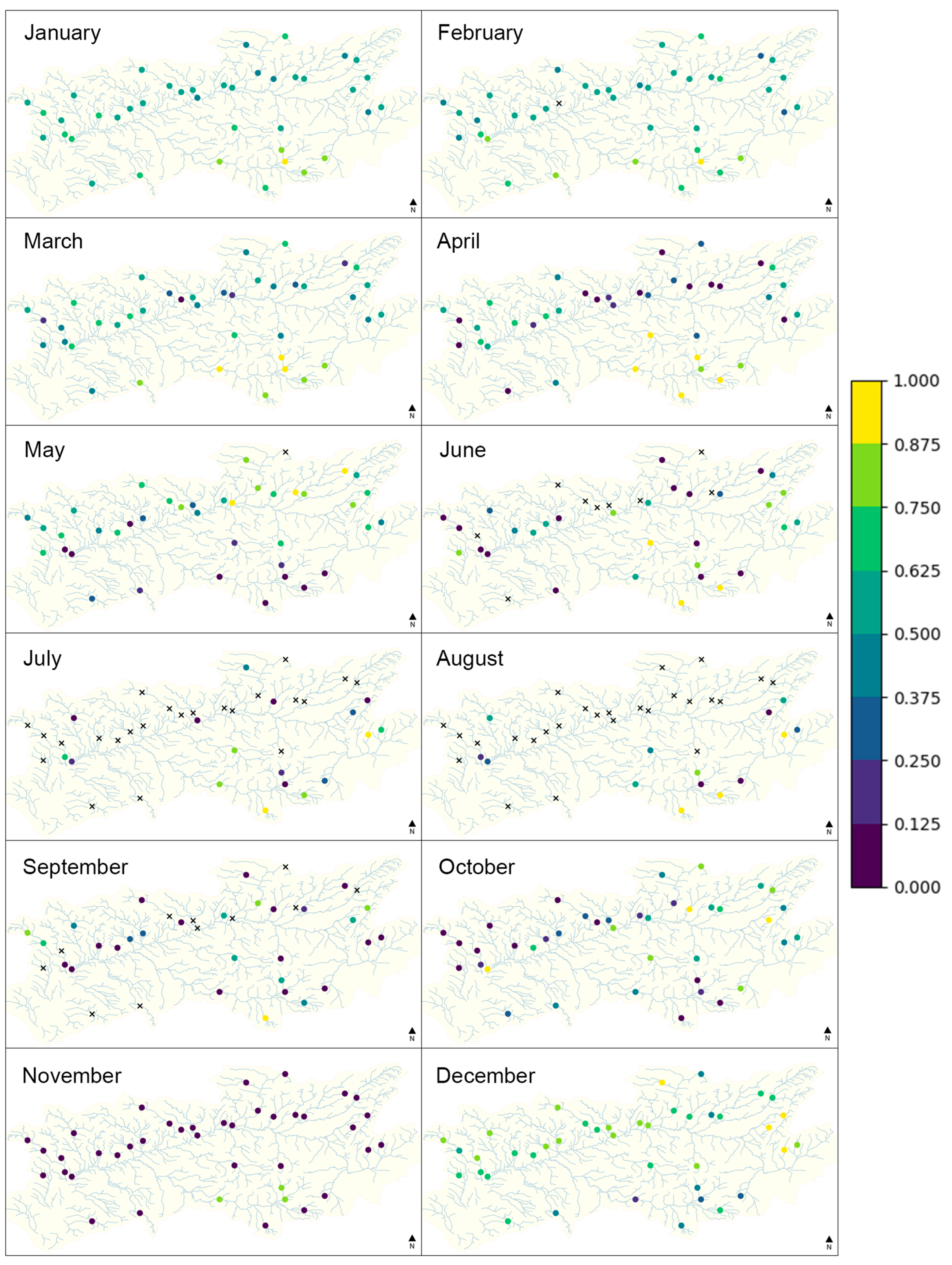
3.1. Correlations between SSI and SPEI

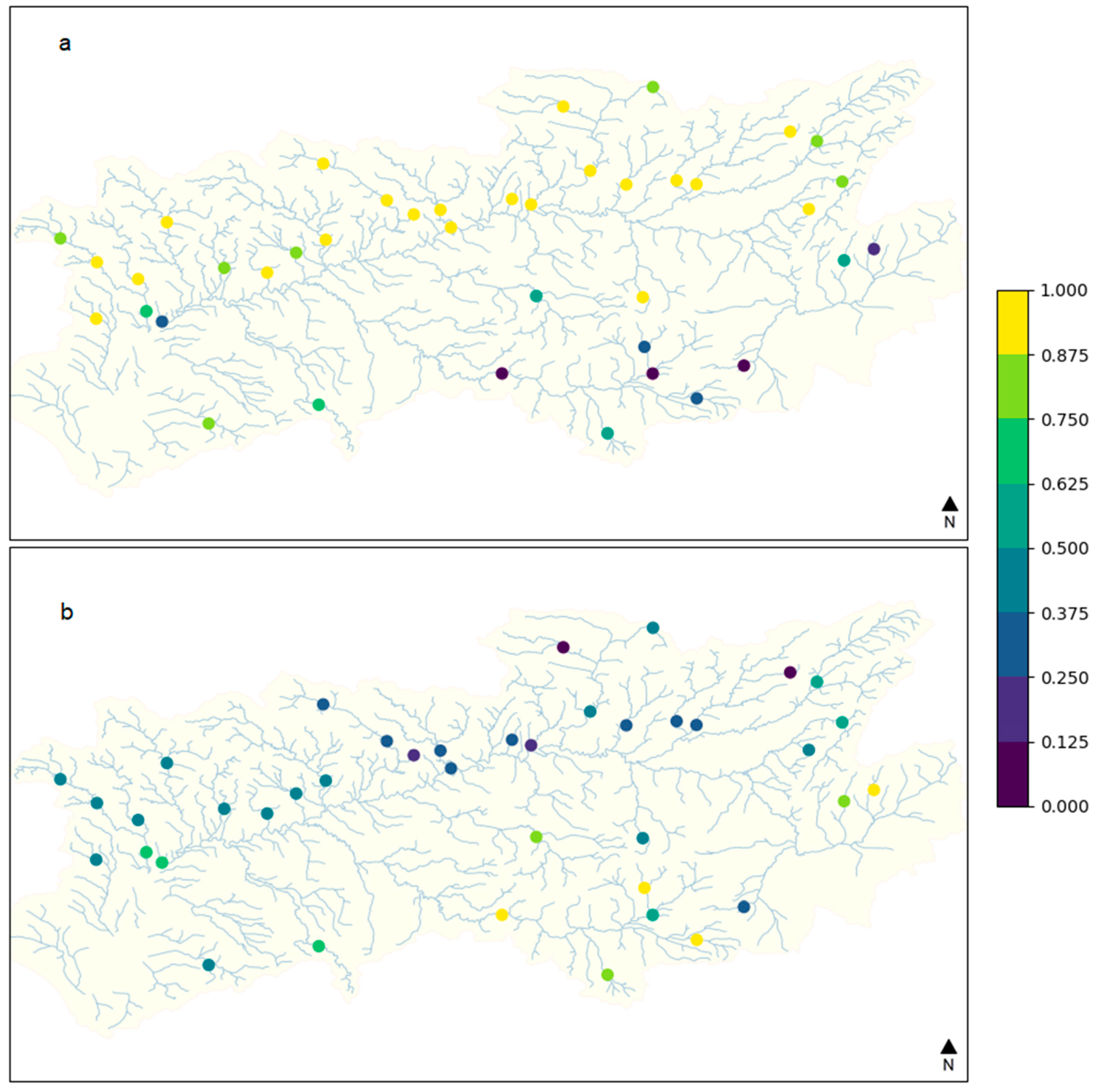
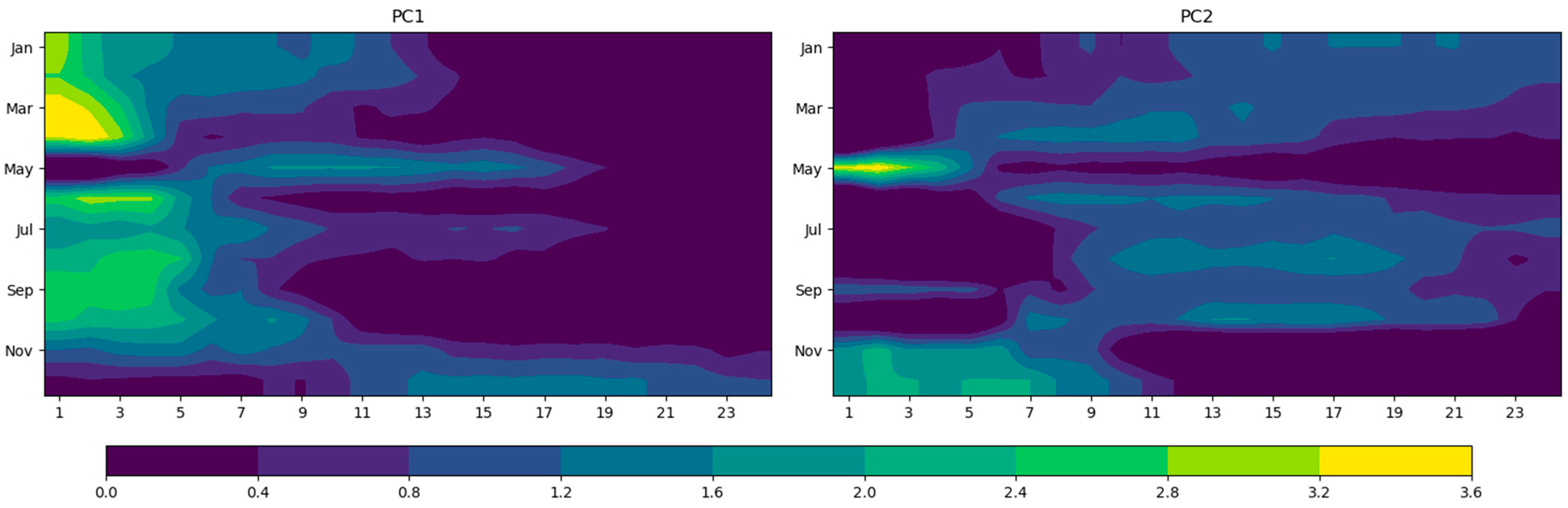
When correlating the indices, it was considered that soil memory could introduce a delay in the correlation values between SPEI and SSI [41]. This situation would be particularly interesting for short accumulation periods. Figure 4 shows the correlation between SPEI and SSI for station 5018 (located to the northeastern area) accounting with different SPEI delays and accumulation periods. As can be seen, correlation decreases as the delay increases in this station for all accumulation periods. The same effect appeared in all stations of the basin. This is in accordance with the results of Koster and Suarez [10], where it is shown that the value of this lag is between 1 and 2 months in arid and semi-arid regions. The fact that the data used in this study are monthly accumulated instead of daily explains that correlations are higher for simultaneous SPEI and SSI series.

Once the effect of soil memory was checked, propagation from meteorological to hydrological drought was analyzed. It was discovered that the studied stations have different behaviors in their correlations. Figure 5 shows the SPEI accumulation period for which correlations between SSI and SPEI reach the maximum value. As can be seen, maximum correlations occur at short accumulation periods (around 2 or 3 months) for most stations. There are, however, several exceptions. Most notably, stations 5019 and 5025, located in the south, and 5032, in the center, show that maximum correlations appear with large accumulation periods of 24 months. This is the first sign of the special treatment that these three stations require, which will be discussed later in this study. This differentiation is required because of their distinct physical characteristics, mainly their catchment area, larger than 4000 km², as shown in Figure 2a.

An interesting part of the basin appears in Sierra Nevada, to the southeast. There are two stations with maximum correlations at 21 and 24 months of accumulation, while the surrounding stations are between 10 and 13 months. Note that the highest altitudes of the whole basin are reached in this area, so water received in these stations comes mainly from meltdown. Thus, in this area, streamflows are not created rapidly after precipitation, they are formed several months thereafter.

Three detailed examples of the evolution of correlation with the accumulation period are shown in Figure 6. Station 5016 is the westernmost station in the study area (Figure 1), and it is located in the header of its sub-basin, so it has no upstream regulation. Its correlation peak appears in the 2-month accumulation period, and it decreases thereafter. The explanation for this behavior is that the catchment area is small and relatively irregular, causing water from precipitation events to rapidly find the stream. Station 5026 is located in the center and southern part of the Guadalquivir basin, and it has one of the largest catchment areas (Figure 1 and Figure 2a). It shows a peak for the 13-month accumulation period. Note that, for this station, a significant part of its inflow comes from Sierra Nevada, which means that its streamflow is delayed and influenced by precipitations-snow-of several previous months. Lastly, station 5035, located in the northwestern part of the basin, is shown here since it presents a particular feature, with a local maximum in the 2-month accumulation period. However, its correlation later grows between the 3 and the 12-month accumulation periods.

3.2. PCA Analysis

When performing the PCA, the first step is to determine the number of principal components retained. In the case of continuous series, two components explain 96% of the total variance. After applying the varimax rotation, the first principal component explains 67.5% of the total variance, while the second component explains an additional 28.5%.

As shown in Figure 7, PC1 mainly represents stations where short-time responses are the most important, while stations where PC2 has the highest loadings are more affected by accumulation periods longer than 9 months. The loadings of every station are shown in Figure 8 for each PC. As only positive score values corresponding to positive loading values have a physical meaning, negative scores and loadings have not been represented in their corresponding Figure to avoid unnecessary confusion.

Principal component loadings show that there is a clear distinction between north and south in the Basin, with Guadalquivir River as the dividing line. Northern stations are generally represented by PC1 (Figure 8a), while southern stations, with some exceptions, present higher PC2 loadings (Figure 8b).

A possible explanation is that tributaries on the northern bank of the Guadalquivir are generally shorter than those on the southern bank. Therefore, shorter accumulation periods dominate in the northern area. On the contrary, the course of rivers in the southern part such as Guadiana Menor, Guadajoz, or Genil is longer, and large accumulation periods gain influence in this area.

The area belonging to Sierra Nevada, south of the basin, is also interesting. Even though there are no reservoirs directly on the mountains, the stations in this area are located at high altitudes, in a mountainous region which includes the highest peaks in the Iberian Peninsula. For Sierra Nevada and Sierra de Segura stations, high PC2 loadings are related to longer accumulation periods. This result is reasonable, since streamflow happens here mostly when snow melts. It is, therefore, realistic to assume that it is highly correlated to precipitation (or snow) from previous months. This result is confirmed with those presented in [42], even though accumulation periods in the latter are larger than in the Guadalquivir basin. However, it is explainable because of the higher altitudes of the studied basin in [42].

In addition to Sierra Nevada, there are other interesting results in the basin. Stations 5035 and 5042, both located close to each other and to the river estuary (Figure 1), do not follow the same trend as other stations in their vicinity. Station 5042 shows medium to high loadings for both principal components since maximum correlations occur here at 11 months (Figure 5), with similar although lower correlation values for 9 and 10 months. Following Figure 7, this is the accumulation period range in which PC1 score is surpassed by PC2 score, so it is logical that this station is represented by both components. However, station 5035 is exclusively represented by PC2, which implies longer accumulation periods despite the fact that the maximum correlation value in this station is reached for an accumulation period of 2 months (Figure 5). This seems to contradict the score results, but it can be explained by looking at the correlation values of each accumulation period for this station in Figure 6. While 2 months is the maximum and the following short accumulation periods present lower correlation values, they rise again between 9 and 12 months, which are the accumulation periods for which PC2 has the maximum scores. Therefore, correlation values of station 5035 are better represented by PC2.

Stations 5019, 5025 (central-southern part of the basin), and 5032 (north-central part of the basin) are not represented by either of the two principal components. Moreover, according to Figure 5, SPEI accumulation periods for maximum correlation are the longest of the basin on these points. As stated before, these stations are particular because they are located in the largest catchment areas in the basin (Figure 2a), showing a different behavior that is not represented by the PC1 or PC2. For this reason, they will be analyzed separately.

In addition to the analysis of the continuous series, another PCA was performed on the twelve monthly series. These twelve PCAs were performed with two principal components each. The percentage of total variance represented by the first two rotated PCs ranges from 66% (September) to 98% (January). The specific value for each month appears in Figure 9 and Figure 10 for PC1 and PC2, respectively. There are some stations where the streamflow dataset had monthly gaps, mostly during the summer months. These gaps are provoked most probably due to errors in the stream gauging stations, due to the low or inexistent streamflow during those months. For such stations, the results of the monthly PCA were not reliable enough, so they were marked with crosses in Figure 9 and Figure 10, and excluded from this analysis.

Figure 11 shows the scores of both principal components regarding the accumulation period. At monthly scale, it is clear that, except for May and December, PC1 is representative of stations with low accumulation periods, while PC2 is related to longer accumulation periods. This is similar to the result that appeared in the continuous series analysis. Figure 9 and Figure 10 show the corresponding loadings for every month.

Generally, monthly principal components follow the same general behavior that appeared in the continuous series analysis. There are, however, two important exceptions: May and December. In May, PC1 represents longer accumulation periods, and PC2 denotes shorter accumulation periods. Moreover, spatial loading distribution is not as clear as in other months. Longer periods appear mostly in Sierra Nevada and the northwestern part of the basin, with shorter periods gaining importance only in some stations in the northeastern part of the basin. This result could be explained by considering that longer periods in May include snowmelt that happened during the spring, together with the normal precipitation increase that occurs in March and April [43]. For December, PC1 explains the south of the basin, which means that longer periods are dominant in this part, although with low scores. Shorter periods, represented by PC2, appear in the northern part of the basin. Since December is the month with the highest precipitation values [18], this result means that precipitation is converted into streamflow shortly after it happens, while mountainous areas accumulate snow that will turn into streamflow in future months. A similar result is discussed in [44], where nival regimes require longer accumulation periods, driven by snow-melt processes.

In order to analyze the differentiated behavior found between meteorological and hydrological droughts in detail, an exhaustive examination of the physical characteristics of the sub-basin has been carried out. To this end, it was studied how PCA results are impacted by the physical characteristics of each sub-basin where stations are located. For PC1 and PC2 separately, all stations with positive loadings are introduced in a multiple linear regression model together with the values of altitude, percentage of permeable soil, and catchment area.

Figure 12 represents how well the stations represented by each PC are adjusted by the linear model. The line represents the perfect adjustment, so the horizontal distance between the line and each point characterizes the residuals. For PC1 (Figure 12a), the regression has R² = 0.71, with p-value = 5.05 × 10⁻⁹. Based on p-values for each variable, shown in

Table 2. p-values of each variable and PC for the multiple linear regression analysis.

Variable	PC1	PC2
Altitude	0.38	7.34 × 10−3
Permeability	0.28	0.70
Catchment area	5.05 × 10−9	3.2 × 10−2

, the only variable that seems to impact the loadings is the catchment area, while permeability and altitude are not statistically significant. This result confirms the hypothesis that stations 5019, 5025, and 5032, not shown in Figure 12, had to be studied separately; due to their exceptionally large catchment area, they can be considered as outliers in the regression analysis. These results are in accordance with the hypotheses studied by Heudorfer and Stahl [45] and van Langen et al. [46].

Concerning PC2, the regression results show R² = 0.73 and p-value = 1.9 × 10⁻² (Figure 12b). According to the p-values of each variable (Table 2), this regression excludes permeability, while altitude is the most significant factor, followed by catchment area.”

4. Conclusions

The relationship between hydrological and meteorological droughts in the Guadalquivir basin has been analyzed using two drought indices, SSI and SPEI, through the correlation analysis.

Two main correlation types have been found in the basin. These types are short-time and long-time correlations. Short time scale correlations, with accumulation periods of maximum correlation ranging generally from 1 to 6 months, appear in the northern part of the basin, comprised mainly by flat areas, or short tributaries basins. In these areas, hydrological drought occurs shortly after the appearance of meteorological drought. In mountain areas, however, longer time scale correlations are present. Here, the snowmelt has a significant influence on the development of droughts. Accumulation periods above 9 months cause the highest correlations between SSI and SPEI. Additionally, there is a differenced behavior that happens in stations located downstream of another close reservoir. For these cases, since their streamflow is regulated, the correlation between streamflow and precipitation is nullified.

Through a PCA with varimax rotation, the basin has been divided into different areas with similar correlation patterns between the SSI and the 1–24 months accumulated period SPEI. The PCA was performed both on the continuous correlation series and separately on each of the monthly correlation series.

The results from the continuous series analysis showed that a first division can be made between North and South of the Guadalquivir River, with few stations showing a differentiating behavior from their neighboring stations. Short accumulation periods dominate the northern part, where tributaries are shorter and streamflow rates are lower, while longer accumulation periods have more influence in the south. The orography is also important in this basin, since accumulation periods presenting maximum correlations in mountainous areas on the southeastern part of the basin are different from those in flat areas. Generally, longer accumulation periods show higher correlation in the former, with the contrary happening in the latter.

The monthly PCA analysis shows that the behavior observed in the continuous series analysis is maintained during each separate month, except for May and December. In May, snowmelt and increased precipitations provoke that the spatial distribution that has been explained is not maintained. Meanwhile, in December, precipitation increases, so streamflows are formed in the flatter areas of the north with short accumulation periods, while the mountainous areas are represented by longer accumulation periods since snow will increase streamflows in later months.

For stations presenting low accumulation periods, catchment area is the most important parameter in order to describe the correlations between PCs and the values of altitude, percentage of permeable soil, and catchment area. Nevertheless, altitude is the variable with highest influence for long accumulation periods. This is confirmed by the spatial distribution of stations in the PCA, with PC2 mostly describing points in mountainous areas.

Results from this study can be useful to understand the mechanism behind hydrological droughts, and the importance of river regulation in its development. However, in this study, there are no data available in the area close to the mouth of the Guadalquivir, to the southwest. This is a protected area and no reservoirs have been built there, resulting in the lack of data for the study. As it is an interesting marshland, it could be the subject of a future study with a different data source, for instance, data from hydrological models. Additionally, similar studies can be performed using data from future climate simulations. The comparison of present and future drought behavior can help foresee and mitigate different impacts of climate change on semi-arid river basins.

References

1. Birkmann, J.; Jamshed, A.; McMillan, J.M.; Feldmeyer, D.; Totin, E.; Solecki, W.; Ibrahim, Z.Z.; Roberts, D.; Kerr, R.B.; Poertner, H.-O.; et al. Understanding human vulnerability to climate change: A global perspective on index validation for adaptation planning. Sci. Total Environ. 2021, 803, 150065. [Google Scholar] [CrossRef] [PubMed]
2. García-Ruiz, J.M.; López-Moreno, I.; Vicente-Serrano, S.M.; Lasanta-Martínez, T.; Beguería, S. Mediterranean water resources in a global change scenario. Earth-Sci. Rev. 2011, 105, 121–139. [Google Scholar] [CrossRef]
3. García-Valdecasas Ojeda, M.; Gámiz-Fortis, S.R.; Romero-Jiménez, E.; Rosa-Cánovas, J.J.; Yeste, P.; Castro-Díez, Y.; Esteban-Parra, M.J. Projected changes in the Iberian Peninsula drought characteristics. Sci. Total Environ. 2021, 757, 143702. [Google Scholar] [CrossRef] [PubMed]
4. Peña-Gallardo, M.; Vicente-Serrano, S.M.; Hannaford, J.; Lorenzo-Lacruz, J.; Svoboda, M.; Domínguez-Castro, F.; Maneta, M.; Tomas-Burguera, M.; El Kenawy, A. Complex influences of meteorological drought time-scales on hydrological droughts in natural basins of the contiguous Unites States. J. Hydrol. 2019, 568, 611–625. [Google Scholar] [CrossRef]
5. López-Moreno, J.; Vicente-Serrano, S.; Zabalza, J.; Beguería, S.; Lorenzo-Lacruz, J.; Azorín-Molina, C.; Morán-Tejeda, E. Hydrological response to climate variability at different time scales: A study in the Ebro basin. J. Hydrol. 2013, 477, 175–188. [Google Scholar] [CrossRef]
6. Vicente-Serrano, S.M.; Domínguez-Castro, F.; McVicar, T.R.; Tomas-Burguera, M.; Peña-Gallardo, M.; Noguera, I.; López-Moreno, J.I.; Peña, D.; El Kenawy, A. Global characterization of hydrological and meteorological droughts under future climate change: The importance of timescales, vegetation-CO2 feedbacks and changes to distribution functions. Int. J. Climatol. 2020, 40, 2557–2567. [Google Scholar] [CrossRef]
7. Yongxiao, C.; Jianping, Y.; Huaibin, W. Relationship between meteorological and hydrological drought in the mountain areas: A study in the upper reaches of Ying River, China. Desalination Water Treat. 2021, 220, 22–35. [Google Scholar] [CrossRef]
8. Álvarez-Garreton, C.; Boisier, J.; Garreaud, R.; Seibert, J.; Vis, M. Progressive water deficits during multiyear droughts in basins with long hydrological memory in Chile. Hydrol. Earth Syst. Sci. 2021, 25, 429–446. [Google Scholar] [CrossRef]
9. Yang, Y.; McVicar, T.R.; Donohue, R.J.; Zhang, Y.; Roderick, M.L.; Chiew, F.H.; Zhang, L.; Zhang, J. Lags in hydrologic recovery following an extreme drought: Assessing the roles of climate and catchment characteristics. Water Resour. Res. 2017, 53, 4821–4837. [Google Scholar] [CrossRef]
10. Koster, R.D.; Suarez, M.J. Soil Moisture Memory in Climate Models. J. Hydrometeorol. 2001, 2, 558–570. [Google Scholar] [CrossRef]
11. McKee, T.B.; Doesken, N.J.; Kleist, J. The Relationship of Drought Frequency and Duration to Time Scales. In Proceedings of the Eighth Conference on Applied Climatology, Anaheim, CA, USA, 17–22 January 1993. [Google Scholar]
12. Vicente-Serrano, S.; Beguería, S.; López-Moreno, J.I. A Multi-scalar drought index sensitive to global warming: The Standardized Precipitation Evapotranspiration Index—SPEI. J. Clim. 2010, 23, 1696–1718. [Google Scholar] [CrossRef]
13. Vicente-Serrano, S.M.; López-Moreno, J.I.; Beguería, S.; Lorenzo-Lacruz, J.; Azorín-Molina, C.; Morán-Tejeda, E. Accurate Computation of a Streamflow Drought Index. J. Hydrol. Eng. 2012, 17, 318–332. [Google Scholar] [CrossRef]
14. Tomas-Burguera, M.; Vicente-Serrano, S.M.; Peña-Angulo, D.; Domínguez-Castro, F.; Noguera, I.; El Kenawy, A. Global Characterization of the Varying Responses of the Standardized Precipitation Evapotranspiration Index to Atmospheric Evaporative Demand. J. Geophys. Res. Atmos. 2020, 125, 17. [Google Scholar] [CrossRef]
15. Mehr, A.D.; Sorman, A.U.; Kahya, E.; Afshar, M.H. Climate change impacts on meteorological drought using SPI and SPEI: Case study of Ankara, Turkey. Hydrol. Sci. J. 2020, 65, 254–268. [Google Scholar] [CrossRef]
16. Zare Abyaneh, H.; Ghabaei Sough, M.; Mosaedi, A. Drought monitoring based on Standardized Precipitation Evaoptranspiration Index (SPEI) under the effect of climate change. J. Water Soil Agric. Sci. Technol. 2015, 29, 374–392. [Google Scholar] [CrossRef]
17. Stahl, K. Hydrological Drought: A Study Across Europe. Ph.D. Thesis, Albert-Ludwigs-University of Freiburg, Freiburg, Germany, 2001. [Google Scholar]
18. Yeste, D.J.; Martin-Rosales, W.; Molero, E.; Esteban-Parra, M.J.; Rueda, F. Climate-driven trends in the streamflow records of a reference hydrologic network in Southern Spain. J. Hydrol. 2018, 556, 55–72. [Google Scholar] [CrossRef]
19. Zhang, X.; Zengchao, H.; Singh, V.; Zhang, Y.; Feng, S.; Xu, Y.; Hao, F. Drought propagation under global warming: Characteristics, approaches, processes, and controlling factors. Sci. Total Environ. 2022, 838, 6021. [Google Scholar] [CrossRef]
20. Yılmaz, M.; Alp, H.; Tosunoğlu, F.; Aşıkoğlu, Ö.L.; Eriş, E. Impact of climate change on meteorological and hydrological droughts for Upper Coruh Basin, Turkey. Nat. Hazards 2022, 112, 1039–1063. [Google Scholar] [CrossRef]
21. Dikici, M. Drought analysis with different indices for the Asi Basin (Turkey). Sci. Rep. 2020, 10, 20739. [Google Scholar] [CrossRef]
22. Chanyang, S.; Park, S.-Y.; Kim, J.-S.; Lee, J.-H. Prognostic and diagnostic assessment of hydrological drought using water and energy budget-based indices. J. Hydrol. 2020, 591, 125549. [Google Scholar] [CrossRef]
23. Salimi, H.; Asadi, E.; Darbandi, S. Meteorological and hydrological drought monitoring using several drought indices. Appl. Water Sci. 2021, 11, 11. [Google Scholar] [CrossRef]
24. Calvache, M.L.; Duque, C.; Pulido-Velázquez, D. Summary Editorial: Impacts of global change on groundwater in Western Mediterranean countries. Environ. Earth Sci. 2020, 79, 531. [Google Scholar] [CrossRef]
25. Wu, J.; Chen, X.; Yao, H.; Gao, L.; Chen, Y.; Liu, M. Non-linear relationship of hydrological drought responding to meteorological drought and impact of a large reservoir. J. Hydrol. 2017, 551, 495–507. [Google Scholar] [CrossRef]
26. Edossa, D.C.; Babel, M.S.; Gupta, A.D. Drought analysis in the Awash River Basin, Ethiopia. Water Resour. Manag. 2010, 24, 1441–1460. [Google Scholar] [CrossRef]
27. Morán-Tejeda, E.; López-Moreno, J.I.; Ceballos-Barbancho, A.; Vicente-Serrano, S.M. River regimes and recent hydrological changes in the Duero basin (Spain). J. Hydrol. 2011, 404, 241–258. [Google Scholar] [CrossRef]
28. Serrano Notivoli, R.; De Luis, M.; Beguería, S.; Saz, M.Á. SPREAD (Spanish PREcipitation At Daily scale). ESSD 2017, 9, 721–738. [Google Scholar]
29. Tomás-Burguera, M.; Beguería, S.; Vicente Serrano, S.M.; Reig-Gracia, F.; Latorre Garcés, B. SPETo (Spanish reference evapotranspiration). Copernic. Publ. 2019, 11, 1917–1930. [Google Scholar]
30. Allen, R.G.; Pereira, L.S.; Raes, D.; Smith, M. Crop Evapotranspiration—Guidelines for Computing Crop Water Requirements; FAO Irrigation and drainage paper 56; FAO—Food and Agriculture Organization of the United Nations: Rome, Italy, 1998. [Google Scholar]
31. Confederación Hidrográfica del Guadalquivir, “S.A.I.H. del Guadalquivir”. 2021. Available online: https://www.chguadalquivir.es/saih/ (accessed on 5 July 2021).
32. Abramowitz, M.; Stegun, I.A. Handbook of Mathematical Functions with Formulas, Graphs, and Mathematical Tables; US Government Printing Office: Washington, DC, USA, 1964.
33. Lorenzo-Lacruz, J.; Vicente-Serrano, S.; González-Hidalgo, J.; López-Moreno, J.; Cortesi, N. Hydrological drought response to meteorological drought in the Iberian Peninsula. Clim. Res. 2013, 58, 117–131. [Google Scholar] [CrossRef]
34. Likens, G.E.; Bormann, F.H. Biogeochemistry of a Forested Ecosystem; Springer Science & Business Media: Berlin/Heidelberg, Germany, 2013. [Google Scholar]
35. Kazemzadeh, M.; Malekian, A. Spatial characteristics and temporal trends of meteorological and hydrological droughts in northwestern Iran. Nat. Hazards 2016, 80, 191–210. [Google Scholar] [CrossRef]
36. Bretherton, C.S.; Smith, C.; Wallace, J.M. An Intercomparison of Methods for finding Coupled Patterns in Climate Data. J. Clim. 1992, 5, 541–560. [Google Scholar] [CrossRef]
37. Demšar, U.; Harris, P.; Brunsdon, C.; Fotheringham, A.S.; McLoone, S. Principal Component Analysis on Spatial Data: An Overview. Ann. Assoc. Am. Geogr. 2012, 103, 106–128. [Google Scholar] [CrossRef]
38. Barreira, S. Differences between Temporal (S-Mode) and Spatial (T-Mode) Principal Component Analysis of Antarctic Sea Ice Monthly Concentration Anomalies: Relationship with Climate Variables. Geophys. Res. Abstr. 2011, 13, EGU2011-146. [Google Scholar]
39. Hannachi, A.; Unkel, S.; Trendafilov, N.; Jolliffe, I. Independent Component Analysis of Climate Data: A New Look at EOF Rotation. J. Clim. 2009, 22, 2797–2812. [Google Scholar] [CrossRef]
40. Vejmelka, M.; Pokorná, L.; Hlinka, J.; Hartman, D.; Jajcay, N.; Paluš, M. Non-random correlation structures and dimensionality reduction in multivariate climate data. Clim. Dyn. 2015, 44, 2663–2682. [Google Scholar] [CrossRef]
41. Khodayar, S.; Sehlinger, A.; Feldmann, H.; Kottmeier, C. Sensitivity of soil moisture initialization for decadal predictions under different regional climatic conditions in Europe. Int. J. Climatol. 2014, 35, 1899–1915. [Google Scholar] [CrossRef]
42. Fang, W.; Huang, S.; Huang, Q.; Huang, G.; Wang, H.; Leng, G.; Wang, L. Identifying drought propagation by simultaneously considering linear and nonlinear dependence in the Wei River basin of the Loess Plateau, China. J. Hydrol. 2020, 591, 125287. [Google Scholar] [CrossRef]
43. Fang, X.; Pomeroy, J.W. Snowmelt runoff sensitivity analysis to drought on the Canadian prairies. Hydrol. Processes 2007, 21, 2594–2609. [Google Scholar] [CrossRef]
44. Oertel, M.; Meza, F.J.; Gironás, J.; Scott, C.A.; Rojas, F.; Pineda-Pablos, N. Drought Propagation in Semi-Arid River Basins in Latin America: Lessons from Mexico to the Southern Cone. Water 2018, 10, 1564. [Google Scholar] [CrossRef]
45. Heudorfer, B.; Stahl, K. Comparison of different threshold level methods for drought propagation analysis in Germany. Hydrol. Res. 2017, 5, 1311–1326. [Google Scholar] [CrossRef]
46. van Langen, S.C.H.; Costa, A.C.; Ribeiro Neto, G.G.; van Oel, R. Effect of a reservoir network on drought propagation in a semi-arid catchment in Brazil. Hydrol. Sci. J. 2021, 66, 1567–1583. [Google Scholar] [CrossRef]
Figure 1. Location of the Guadalquivir River Basin in the southern Iberian Peninsula. Designation of reservoir stations and their spatial distribution in the Guadalquivir River basin. Altitude in meters is represented with a color scale, and longest tributaries and main mountain ranges are located in the map.
Water 14 02849 g001
Figure 2. (a) Catchment area of each station in km2, capped at 4000 km2. (b) Percentage of permeable soil in the catchment basin of each station.
Water 14 02849 g002
Figure 3. Flowchart of the proposed methodology.
Water 14 02849 g003
Figure 4. Correlation between SPEI and SSI for station 5018 with different SPEI delays and accumulation periods.
Water 14 02849 g004
Figure 5. SPEI accumulation period for which correlations between SSI and SPEI reach the maximum value. Additionally, six stations marked in blue show their reference code because they are analyzed in detail in this section.
Water 14 02849 g005
Figure 6. SPEI-SSI correlation for different SPEI accumulation periods in stations 5016, 5026, and 5035.
Water 14 02849 g006
Figure 7. Principal component scores (varimax rotated) for the complete correlation series between SPEI and SSI for different SPEI accumulation periods.
Water 14 02849 g007
Figure 8. Loadings of (a) PC1 and (b) PC2 of the continuous series analysis.
Water 14 02849 g008
Figure 9. PC-1 loadings for the monthly series. Crossed stations indicate insufficient data for that monthly analysis.
Water 14 02849 g009
Figure 10. PC-2 loadings for the monthly series. Crossed stations indicate insufficient data for that monthly analysis.
Water 14 02849 g010
Figure 11. Scores of the two principal components obtained in the monthly series analysis for each accumulation period (1–24).
Water 14 02849 g011
Figure 12. Comparison between observed values (dots) against adjusted values (line) of the linear regression for (a) PC1 and (b) PC2.
Water 14 02849 g012