Sensitivity of Empirical Equation Parameters for the Calculation of Time of Concentration in Urbanized Watersheds

Abstract

The time of concentration is the time it takes a drop of water in a basin to travel from the most distant point to the outlet, and is one of the most important parameters, along with the morphometric characteristics, for determining the design flow rate in rainfall-runoff models. This study aims to determine the sensitivity of the parameters included in different equations for the calculation of the time of concentration. A case study was conducted on small, urbanized watersheds in the city of Montería, Colombia. The study uses information obtained through field work using GPS equipment and electronic total station, supplemented by geographic information contained in the city drawings of the local sewage company, which includes data on elevations above sea level with sub-metric precision. The time of concentration determined by the 12 empirical equations was compared to the results obtained from the equation proposed by the Natural Resources Conservation Service (NRCS), which was considered as a baseline formulation for the intricacy of calculation. Based on this comparison, it was found that the Carter equation is the one that best fits the results obtained from the NRCS equation because it displayed highly significant goodness of fit values. Even though the equations by Kirpich, Ventura, California Culvert Practice, Simas-Hawkins and TxDOT provide a relatively good fit compared to other empirical equations, they tend to over-estimate time of concentration values, which could lead to the under-estimation of the design flow rates. For this reason, sensitivity analysis of the parameters of these equations represents an alternative for improving the calculation of the time of concentration. The current research analyses deepen the influence of some parameters in the estimation of time of concentration. The research can also be used by designers and engineers in the city of Montería, Colombia, as an important reference to compute time of concentrations in urbanized watersheds.

1. Introduction

In order to design hydraulic structures to manage runoff from rainfall, it is essential to determine the morphometric parameters and the time of concentration of the water basins [1]. In hydrology studies, the time of concentration [2,3,4] is used to estimate the maximum flow rate by means of rainfall-runoff models, from which the maximum flow rate of design for sizing of the hydraulic structures is determined [5].

The time of concentration is defined as the time it takes a drop of water to travel from the most distant point to a determined drainage outlet [6,7], which is equivalent to the minimum time required for the entire basin to feed water to the drainage outlet [8].

Determination of the time of concentration requires the interpretation both of rainfall records [9] of hydrological stations located within a basin, and of outflow records from a station located at the basin’s drainage outlet. This information is generally obtained from basins that are equipped with adequate instrumentation.

When the above information is not available, designers use equations based on the morphometric parameters of the water basins, such as the slope and length of the watercourse and the type of cover on the basin’s ground. Such equations focus on determining the flow rate [10], and have been developed from basins equipped with instrumentation in Europe and the United States [3,11]. Adequate selection of these equations is crucial in order to avoid over and under-estimating time of concentration values, which would lead to over or under-estimating the maximum flow rates of design for the hydraulic works. Some of the equations used to determine the time of concentration include those by: Témez, William, Kirpich, California Culvert Practice, Giandotti, S.C.S., Ventura-Heron, Brausby-William, Passini, Izzard, Federal Aviation Administration, Morgali and Linsley, Aron and Erborge [12]. Use of these equations depends on the morphometric features of the basins [13].

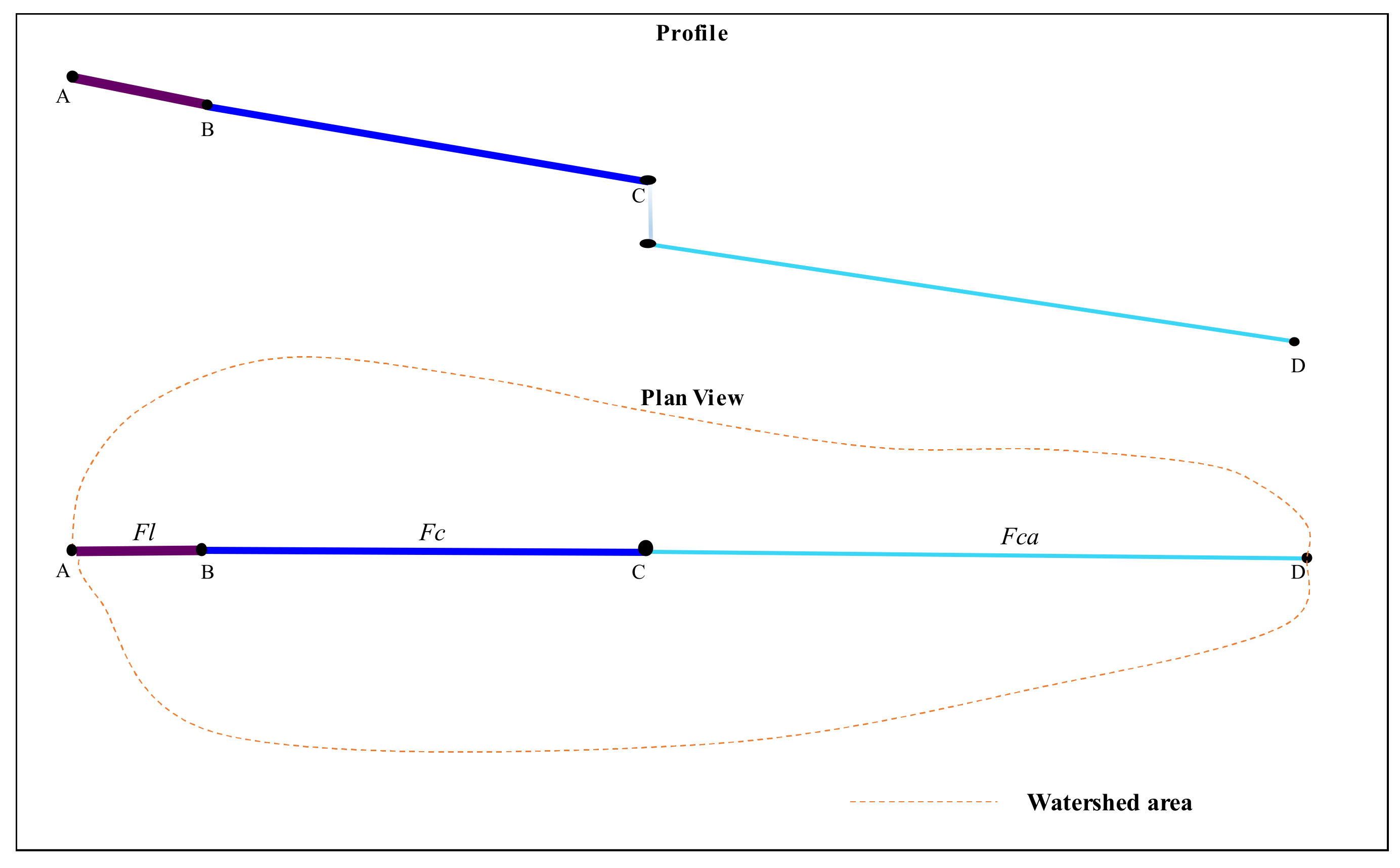
The Natural Resources Conservation Service (NRCS) proposed a formula that is almost fully based on physics to estimate the time of concentration; the formula requires detailed input information for the calculation. The equation proposed by the NRCS is based on determining the travel time for sheet, concentrated and channel flow conditions [14]. Figure 1 presents the plan and side views of the locations where these three types of flows occur. Sheet flow (F_l) occurs at the headwaters of a basin, concentrated flows (F_c) arise immediately after the sheet flow, and channel flow (F_ca) takes place in the drainage channel. 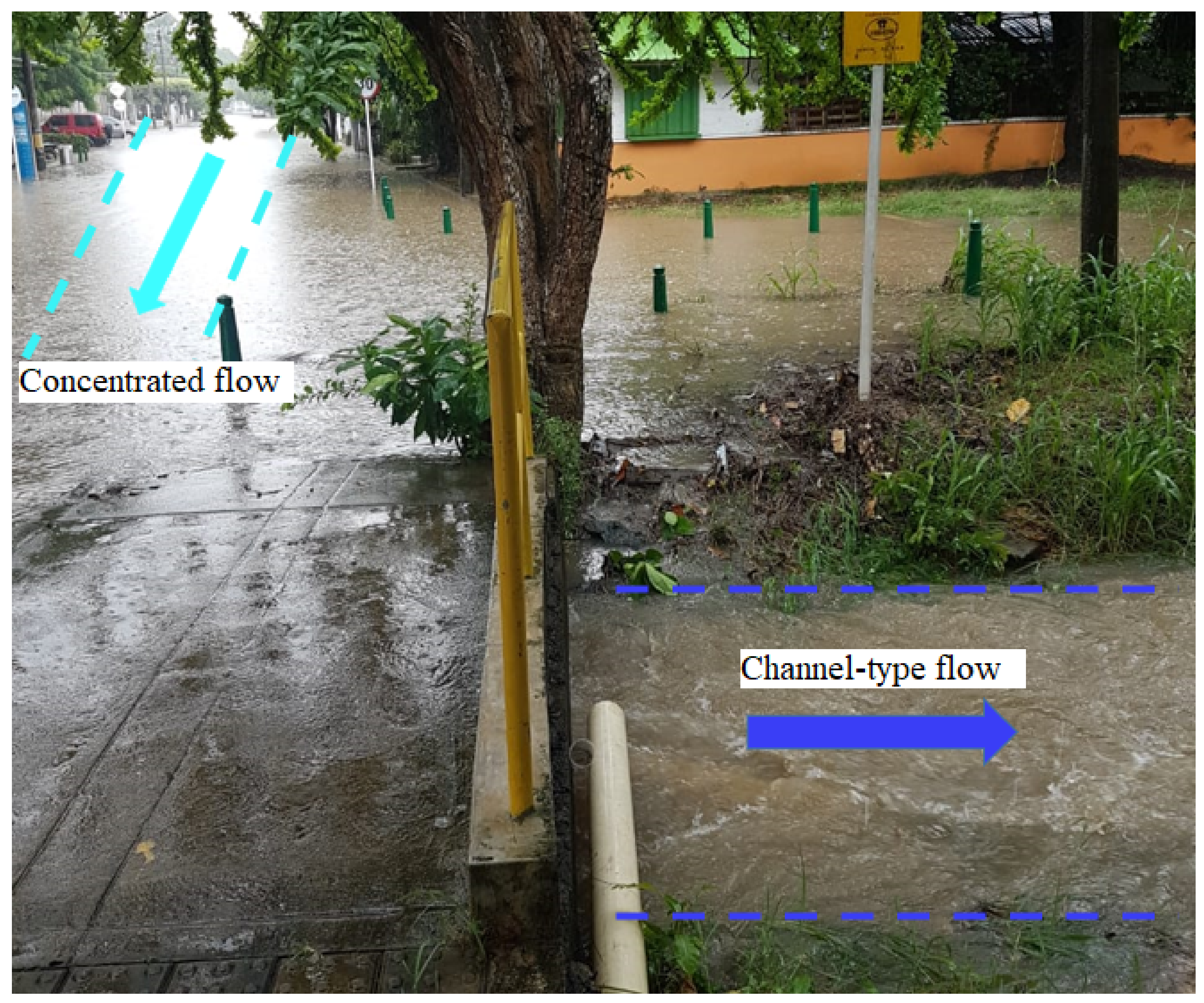Figure 2 displays the differences between the concentrated flow and the channel-type flow, using as reference the behavior of one of the small watersheds of the study following a rainfall event.

In order to improve the characterization of the small urban watersheds and their watercourses, local drawings were used containing elevation data with precision of up to one centimeter, produced from topographic measurements performed by the company responsible for local basic sanitation. Topographic measurements were also made in the field to enable the instrumentation of the main watercourses, providing reliable values for the calculation of the time of concentration, primarily with the baseline equation.

This study aims to determine the sensitivity of the parameters of the empirical equations for the calculation of the time of concentration, using the small watersheds located in the city of Montería, Colombia. The values of time of concentration obtained from the empirical equations are compared to the equation almost fully based on physics developed by the NRCS (called here the baseline equation). This research presents the expression to compute the sheet flow using the NRCS equation in the metric system to avoid confusion in future developments. In addition, it can be used for engineers and designers in the city of Montería, Colombia, to select a priori the best empirical equation to calculate time of concentration of urbanized watersheds.

2. Case Study

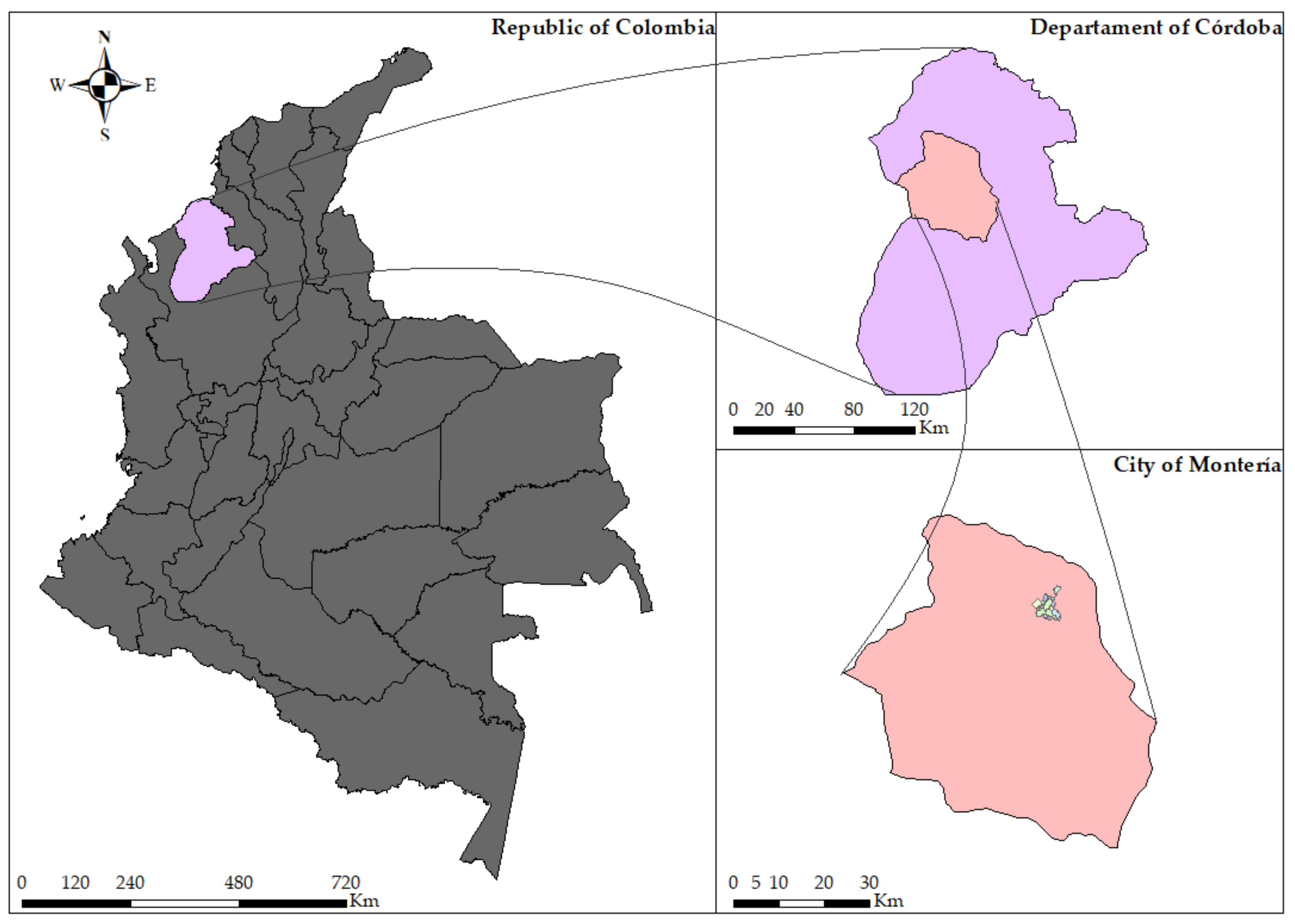
The small urban watersheds of the study are located in the city of Montería, department of Córdoba, Colombia (see Figure 3). It covers an area of approximately 3142 km² and its topography is basically flat with a few elevations. The city is surrounded by numerous creeks and streams, and the city’s main water source is the Sinú River. The region has a rainy season between April and September and a dry season between December and April. The city of Montería has an average slope of 0.2%, and a rainfall drainage system that starts out on the streets as a concentrated flow, and whose superficial runoff is subsequently fed into a drainage channel.

The small watersheds of the study and their respective main watercourses were identified beforehand by means of a geographic information system, performing altimetric tracking in Google Earth, which enabled identifying the perimeters and areas of the urban watersheds, and planimetric tracking, which enabled establishing the layout of the main watercourses.

Afterwards, given that the average topographic slope of the city is flat, adjustments were made to the polygons of small watersheds that had been previously delimited in Google Earth, because the measurement precision of this geographic information is only up to one meter, which creates uncertainty as to the actual perimeter of the small watersheds of the case study. These parameters were adjusted based on the city drawings of the sewage network of the city of Montería, which were provided by the municipal basic sanitation service operator and which contain the elevations above sea level at the city’s main street intersections.

First, the paths followed by the sheet flow and concentrated flow were identified, and afterwards a topographic survey was performed in order to obtain precise information on the magnitudes of the geometric and hydraulic parameters of the drainage channels (channel flow). Field work was also performed to identify the channel sections with homogeneous cover materials, finding that the geometry of the cross-section is typical, and that the longitudinal slope is constant. Information on the channels was obtained using equipment such as: electronic total station, a Topcon high-precision level, and RTK Trimble GPS technology equipment.

Following the selection of the small watersheds of the study and their respective main watercourses, calculations were performed of the morphometric parameters to be used in the study.

3. Materials and Methods

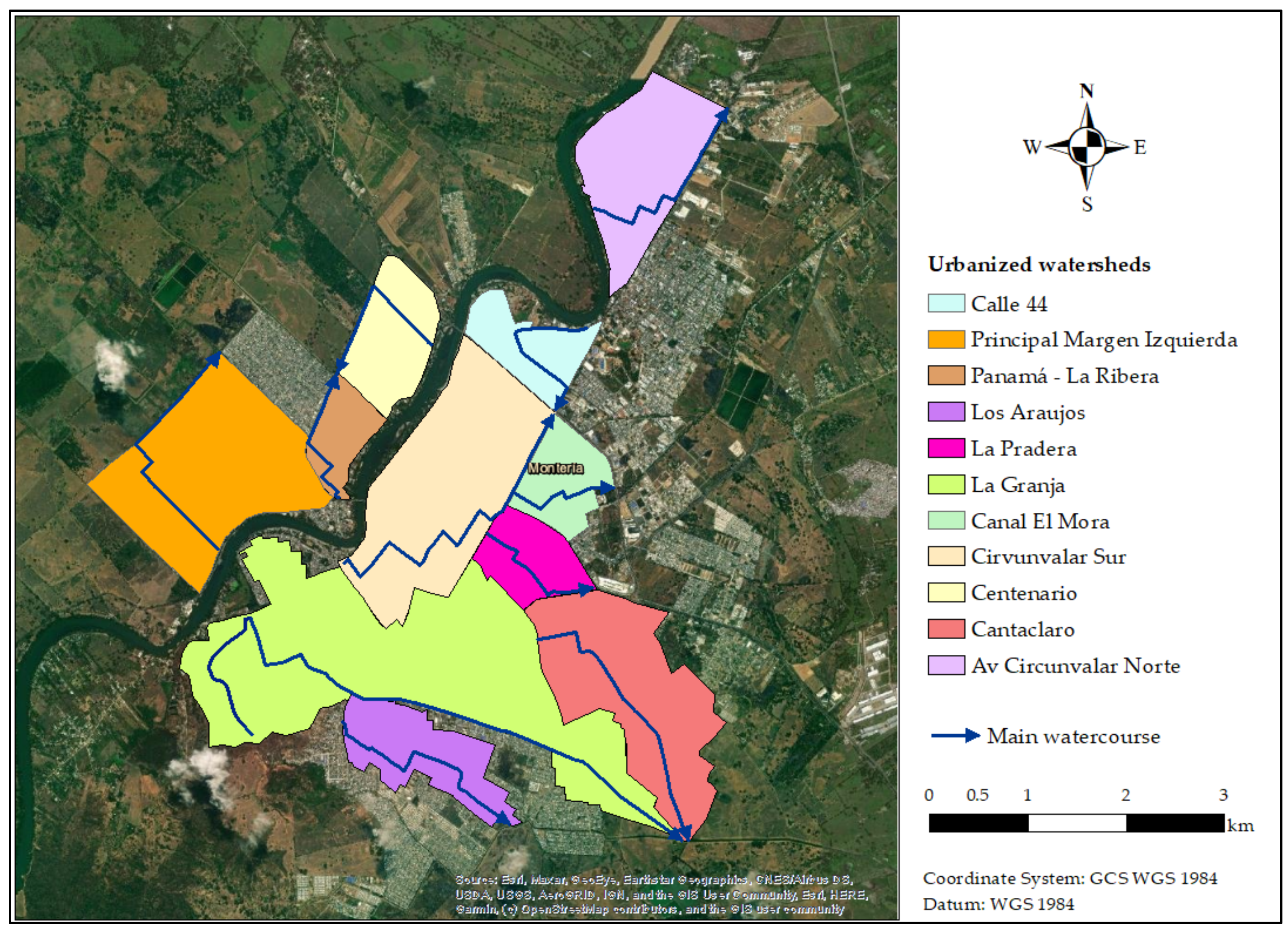
The research process began by determining the small urban watersheds in the area of the study, which were delimited and adjusted for the effects of calculating the morphometric, rainfall and ground cover parameters. Lastly, the main channels were selected, calculating their respective hydraulic and geometric parameters. Figure 4 displays the small watersheds of the study and their corresponding watercourses.

Table 1. Morphometric parameters of the small watersheds of the study and hydraulic parameters of the main watercourse.

Item	Basin	Ac (km2)	Ls (km)	S (m/m)	ΔH (m)	n	P2	C	CN
1	Principal Margen Izquierda	2.83	2.73	0.00060	1.65	0.021	78.19	0.68	84
2	Panamá-La Ribera	0.53	1.56	0.00112	1.75	0.015	78.19	0.88	98
3	Centenario	1.00	1.79	0.00087	1.57	0.015	78.19	0.71	86
4	Los Araujos	1.12	2.41	0.00122	2.94	0.015	78.19	0.88	98
5	La Granja	5.52	6.81	0.00083	5.62	0.023	78.19	0.76	90
6	Cantaclaro	2.52	2.91	0.00110	3.21	0.021	78.19	0.77	90
7	El Mora	0.75	1.19	0.00199	2.36	0.017	78.19	0.88	98
8	Av Circunvalar Sur	3.00	3.56	0.00135	4.80	0.015	78.19	0.88	98
9	Calle 44	0.77	1.78	0.00225	3.99	0.015	78.19	0.88	98
10	Av Circunvalar Norte	1.72	2.18	0.00164	3.57	0.021	78.19	0.64	82
11	La Pradera	0.74	1.44	0.00130	1.86	0.015	78.19	0.88	98

presents the morphometric features of the small watersheds of the study. Their areas (A_c) are between 0.53 and 5.52 km², with a minimum watershed slope (S) of 0.00060 m/m and a maximum slope of 0.00225 m/m, which are consistent with the local topographic conditions. The review of ground cover results indicates that urbanized cover is predominant in terms of the runoff coefficient (C) and the weighted curve number (CN). ΔH is a different elevation in a main watercourse. P₂ is the maximum daily precipitation associated to a return period (Tr) of 2 yr. Lastly, Manning’s roughness coefficient (n) highlights that most watercourses are covered in concrete, which increases the runoff flow rate.

Once the information required for calculation of time of concentration was acquired, the results obtained using the twelve empirical equations were compared to those of the equation developed by the NRCS. The equation that is almost fully based on physics developed by the NRCS is expressed as follows:

$$Tc=T_{fl}+T_{fc}+T_{fca}$$

(1)

where Tc = Time of concentration (h), and m = Number of branches.

The equations were adjusted and presented under the conditions of the International System, which is not published.

The travel time for the sheet flow (F_l) was calculated based on Manning’s roughness coefficient (n), the length and slope of the watercourse and the maximum precipitation of design associated to a two-year return period. The following is the expression used for the calculation:

$$T_{fl}=\frac{0.002886{\left(n{L}_{fl}\right)}^{0.8}}{{\left(P_2/1000\right)}^{0.5}{S}_c^{0.4}}$$

(2)

where T_fl = Sheet flow travel time (h), L_fl = Sheet flow length (m), n = Manning’s roughness coefficient, P₂ = Maximum precipitation in 24 h for a 2-year return period (mm), and S_c = Average watercourse slope (m/m).

The formula for the travel time of the concentrated flow (F_c) assumes that the sheet flow becomes a superficial concentrated flow. The average velocity of this flow is determined based on the following expressions:

For paved surfaces,

$$V=6.1976 \sqrt{S_c }$$

(3)

For unpaved surfaces,

$$V=4.919 \sqrt{S_c}$$

(4)

Once the estimated average velocity is calculated, the travel time of the concentrated flow is calculated using the following expression:

$$T_{fc}=\frac{L_{fc}}{3600V}$$

(5)

where T_fc = Concentrated flow travel time (h), L_fc = Concentrated flow length (m), and V = Average velocity (m/s).

Lastly, the travel time for the channel-type flow (F_ca) is calculated for open channels with defined hydraulic characteristics in the cross-section. Manning’s equation or the information of the profile of the water surface is used to estimate the average flow velocity.

$$V=\frac{R^{2/3} S_c^{1/2}}{n}$$

(6)

where V = Average velocity (m/s), r = Hydraulic radius (m), S_c = average watercourse slope (in this case corresponds to the hydraulic slope of the channel) (m/m), and n = Manning’s roughness coefficient.

Based on the concentrated flow travel time equation, the channel flow travel time is calculated.

$$T_{fca}=\frac{L_{fca}}{3600V}$$

(7)

where T_fca = Channel flow travel time (h) and L_fca = Channel flow length (m).

For analysis, the NRCS formulation is considered as the baseline equation.

In this study, 12 empirical equations were used, which are listed in

Table 2. Methods to be compared to the baseline equation.

No.	Equation	Formula	Description and Reference
1	Kirpich Equation [15]	$Tc=0.0663 {\left(\frac{L_s^2}{S_c}\right)}^{0.385}$	Kirpich (1940), calibrated two empirical models to estimate the time of concentration in small basins in Pennsylvania and Tennessee, with areas between 0.4 and 45.3 ha and average slopes between 3% and 10%. Researchers [6] demonstrated that this method tended to under-estimate Tc by 75% in urbanized basins with areas between 8 and 16 km2, predominantly with channel flows. Researchers [16] demonstrated that using this equation in basins with areas between 17.35 and 598 km2, and average slope between 0.0173 and 0.1029 m/m produced smaller positive biases (mean error of 16.8 h and standard deviation of 37.1%).
2	Millers Equation [17]	$Tc=1.7833\left[\frac{n1000L_s^{0.333}}{{\left(100S_c\right)}^{0.2}}\right]$	Method developed from the nomogram of sheet, concentrated and channel flows published by the Institute of Engineers of Australia (IEA, 1977), [12]. The authors demonstrated that predictive variables with most influence in the calculation of time of concentration were the length of the main watercourse, with values between 8 and 431 km, and the average slope of the main watercourse, with values ranging between 0.00078 and 0.01687 m/m, finding the smallest biases at standard deviation values of less than 20% and mean errors of less than 2 h.
3	California Culvert Practice, [18]	$Tc=0.951L_s^{1.155}\Delta H^{-0.385}$	Method developed by the California Roads Division (1960) for small mountainous basins in California [13] and data obtained from small basins in the USA with areas of less than 40.47 km2 [11]. This is consistent with the results obtained by [19], which estimated the time of concentration in 46 basins of the Po River with areas between 56 and 1.588 km2 and slopes in mountainous terrains ranging between 0.022 and 0.268 m/m. The results displayed values of MSE = 8.21 h, which in general moderately under-estimate the values of Tc, which is neither the best nor the worst result.
4	Carter Method [20]	$Tc=0.0977L_s^{0.6}{S}_c^{-0.3}$	Method developed for urban watersheds with areas of less than 20.8 km2 and channels of lengths of less than 11.3 km (Sharifi & Hosseini, 2011). It is recommended for basins whose main watercourse has natural channel flows between 0.013 and 0.025, [5]. Ref. [11] indicates that this equation was developed based on data from urban watersheds.
5	Federal Aviation Agency method [21]	$Tc=\frac{0.0165626\left(1.1-\mathrm{C}\right)1000L_s^{0.5}}{{\left(100S_c\right)}^{0.333}}$	Developed by engineers in the US based on drainage of air fields [5]. It is widely used for urban sheet flow [12]. Developed primarily for sheet and concentrated flows, [13] used this equation in five water basins that include several sub-basins within them, with slopes ranging between 0.044 and 0.091 m/m. It was found that this and several other equations has lower values in all the assessment criteria, producing inaccurate estimates (MSE = 0.499 h).
6	NRCS equation, kinematic wave method [22]	$Tc=0.0015476\frac{L_S{}^{0.6}}{S_c{}^{0.3}}$	This method is widely used in paved areas, although it was initially used for concentrated flow and channel flow, and is based on the ratio between the intensity and duration of the rainfall associated with a 2-year return period. Additionally, the method was developed to avoid the iterative process of the original formula for the kinematic wave method. When [16] used this equation in basins with average slope between 0.0173 and 0.1029 m/m, they found a bias of less than 10%, with mean error of 1 min.
7	TxDOT method [23]	$Tc=0.369986\left(1.1-C\right)L_s^{0.5}{S}_c{}^{-0.333}$	It is the result of a modification to the FAA’s method (FAA, 1970) [24]. The Texas Department of Transportation (TxDOT) adopted the above methodology in its hydraulic design manual to estimate the Tc in basins in the Texas region [10]. Ref. [25] used this equation to compare the value of Tc to the travel time results in a testing strip for runoff by thrust, from which they developed an equation. They concluded that the TxDOT method tends to over-estimate the value of Tc, producing lower results in clay, asphalt and concrete surfaces, with the highest result in grass cover.
8	Chow’s Model [26]	$Tc=0.1602 \frac{L_s^{0.64}}{S_c{}^{0.32}}$	Equation developed for 20 rural basins rurales in the United States in which the drainage area ranged between 0.01 and 18.5 km2 and the slope of the main watercourse was between 0.0051 and 0.09 m/m. In the same basin of the study, [19] found similar performance between the equation of the California Culvert Practice and the equation of Chow’s Model, with a value of MSE = 7.21 h.
9	Bransby-Williams method [27]	$Tc=0.605 \frac{L_s}{{\left(100S_c\right)}^{0.2 }A{c}^{0.1}}$	Williams (1922) conducted a study on flood discharges in India and Haktanir and Sezen (1990) developed his methodology by means of regression analysis using data from basins located in Turkey [11]. This method is based on experimental use for water basins with drainage areas of less than 129.5 km2 and dominated by channel flow [19]. Ref. [1] used this equation in basins that were similar in terms of total area and urbanization, but where the slope of the different types of flow was different, which apparently affects the equation’s performance.
10	Simas-Hawkins, [28]	$Tc=\frac{0.322A^{0.594}}{L_s^{0.594}{S}_c{}^{0.15}}{\left[\frac{\mathrm{25,400}}{CN}-254\right]}^{0.313}$	Method developed in 168 basins in the United States with areas between 0.001 and 14 km2. A study by [11] used 30 empirical methodologies in one water basin to calculate Tc. Of these equations, the Simas-Hawkins was classified in the group of appropriate equations for natural basins.
11	Ventura-HEC-RAS equation [2]	$Tc=0.067 \frac{L_s^{1.155}}{{\left(\frac{\Delta H}{1000}\right)}^{0.385}}$	This equation applies to small basins [2]. The authors found that in one of the basins of the study, which was sub-divided into 6 sub-basins with slopes ranging between 0.002627 and 0.024079 m/m and length of the main watercourse between 52.389 and 13.345 km, the Venturas method yielded the second-best results with a value of MSE of 2 h. This equation is used for channel flows.
12	Kerby Equation [29]	$Tc=0.02399{\left(\frac{1000n{L}_s}{S_c^{0.5}}\right)}^{0.467}$	This equation can be used for urban drainage lower than 4 ha and slopes under 1%. Commontly, this equation can be used to compute concentrate flow type.

.

Statistical analysis was performed based on the Tc values produced by the baseline equation and by the empirical equations, using analysis of variance (ANOVA). Then Dunnet’s test of multiple comparisons of means was used to select the equations whose Tc is similar to the times of concentration calculated using the baseline equation with a 5% significance level. However, the method used to select the equation that is best suited for the conditions of the basins of the city of Montería, Córdoba was multiple linear regression analysis, using as decision criteria the coefficient of determination (R²) and the mean square error (MSE).

In order to observe the behavior of the Tc calculated values, sensitivity analysis was conducted in four stages.

• The first sensitivity analysis focused on finding the variability of the Tc value calculated by means of the baseline equation by calculating the maximum precipitation in 24 h associated with the 2-year return period, as proposed by the different authors cited in [14,30], who recommend the use of distribution methods, from among which GEV, Log Pearson Type III and Pearson Type III were selected. The result was compared to the value used as reference (Gumbel) [31]. This value is necessary in order to calculate the sheet flow travel time.
• The second sensitivity analysis focused on the variability of the roughness coefficient used in the baseline equation to calculate sheet flow and concentrated flow travel time. To this effect, analysis was performed using the values defined as the minimum, normal and maximum values depending on the type of channel and its description. After recalculating the travel times and the time of concentration, statistical analysis was performed to assess the sensitivity of this variable compared to the empirical equations.
• The third sensitivity analysis was performed by calculating the time of concentration value using the baseline equation, initially without considering the sheet flow travel time, and afterwards without considering the concentrated flow travel time. The obtained values were compared to the values calculated by the different equations to estimate Tc, using MSE and R² as the criteria for comparison. The empirical equations used for the comparison were those that did not display significant differences in the statistical analysis.
• The fourth and last sensitivity analysis focused on verifying the behavior of the empirical equations as a function of variations in the length of the main watercourse and the ground cover of the different urban watersheds. The equations selected for this analysis were those that did not display significant differences compared to the baseline equation according to Dunnet’s test. It should be noted that sensitivity to the two variables mentioned above was not assessed for all the selected equations, either because such variables were not included or were not relevant in the equations. Lastly, time of concentration was calculated using the selected equations, and the results obtained were compared to the values of the baseline equation. The variation found in the results obtained in this analysis was assessed by means of MSE.

4. Results

4.1. Determination of the Time of Concentration

Table 3. Travel time and Tc of the baseline equation.

Watercourse	Travel Time (h)			Tc (h)
	Sheet Flow	Concentrated Flow	Channel Flow
Principal Margen Izquierda	0.09	1.16	0.60	1.85
Panamá-La Ribera	0.16	0.78	0.18	1.12
Centenario	0.18	0.86	0.26	1.30
Los Araujos	0.09	0.45	0.29	0.83
La Granja	0.06	1.78	1.35	3.19
Cantaclaro	0.13	0.47	0.42	1.01
El Mora	0.16	0.52	0.08	0.76
Av Circunvalar Sur	0.10	0.69	0.36	1.15
Calle 44	0.13	0.67	0.10	0.89
Av Circunvalar Norte	0.12	1.02	0.18	1.32
La Pradera	0.15	1.08	0.07	1.30

displays the Tc estimated using the baseline equation of the NRCS for each type of flow.

Table 4. Tc calculation (h) by empirical methods.

Item Basin		Empirical Equations
		1 *	2 *	3 *	4 *	5 *	6 *	7 *	8 *	9 *	10 *	11 *	12 *
1	Principal Margen Izquierda	2.50	0.89	2.50	1.65	0.93	5.02	3.05	3.27	2.61	3.36	2.52	0.89
2	Panamá-La Ribera	1.27	0.48	1.28	0.98	0.30	1.94	0.97	1.87	1.55	0.79	1.29	0.51
3	Centenario	1.56	0.53	1.57	1.15	0.62	2.40	2.03	2.22	1.77	2.09	1.58	0.58
4	Los Araujos	1.73	0.55	1.73	1.24	0.36	2.67	1.18	2.41	2.20	0.93	1.75	0.61
5	La Granja	4.47	1.29	4.48	2.60	1.05	10.18	3.44	5.30	5.72	2.34	4.51	1.34
6	Cantaclaro	2.08	0.82	2.08	1.43	0.62	4.18	2.02	2.81	2.50	2.30	2.10	0.80
7	El Mora	0.83	0.46	0.83	0.70	0.21	1.41	0.70	1.31	1.02	1.04	0.84	0.42
8	Av Circunvalar Sur	2.24	0.61	2.25	1.52	0.42	3.49	1.39	2.99	2.88	1.31	2.27	0.72
9	Calle 44	1.08	0.44	1.08	0.86	0.25	1.63	0.83	1.63	1.49	0.82	1.09	0.46
10	Av Circunvalar Norte	1.43	0.68	1.43	1.07	0.64	2.80	2.10	2.05	1.79	2.59	1.44	0.63
11	La Pradera	1.13	0.45	1.14	0.89	0.27	1.72	0.89	1.69	1.35	0.99	1.14	0.48

Note: * Equations are identified as shown in Table 2.

displays the time of concentration values estimated by the 11 empirical equations.

4.2. Statistical Analysis

Analysis of variance (ANOVA) under a fully randomized block design enabled determining whether or not there were significant differences between the times of concentration calculated by each of the proposed models.

Table 5. Analysis of variance for the times of concentration.

Source	GL	SS	MS	Fo	Fc	p-Value	Decision
Times of concentration	12	87.45	7.29	17.15	1.8337	8.1295 × 10−21	Reject H0
Micro-basins	10	98.82	9.88	23.26	1.9105	1.0166 × 10−23	Reject H0
Error	120	50.98	0.42
Total	142	237.25

displays the formal hypothesis test, where Fo = 17.15, p value below 0.0001, to test the hypothesis of the equality of the times of concentration obtained by each of the proposed equations for calculation of the time of concentration (treatments). Additionally, a hypothesis test was performed with Fo = 23.26 and a value of p < 0.0001 for the block effect (micro-basins).

Given that the analysis of variance found significant differences between the Tc of the proposed equations, Dunnet’s test of comparison of means was then performed in order to determine which equations display significant differences in terms of Tc compared to the baseline equation. The results are displayed in

Table 6. Comparison of means using the Dunnett Test.

Hypothesis	Estimate	Standard Error	t Value	Pr (>|t|)	Decision
Carter vs. NRCS = 0	−0.06	0.28	−0.21	0.83	Do not reject H0
Chow’s vs. NRCS = 0	1.17	0.28	4.19	0.00	Reject H0
California Culvert Practice vs. NRCS = 0	0.51	0.28	1.84	0.07	Do not reject H0
FAA vs. NRCS = 0	−0.74	0.28	−2.95	0.01	Reject H0
Simas-Hawkins vs. NRCS = 0	0.35	0.28	1.25	0.21	Do not reject H0
Kerby vs. NRCS = 0	−0.66	0.28	−2.38	0.02	Reject H0
Kirpich vs. NRCS = 0	0.51	0.28	1.82	0.07	Do not reject H0
Miller vs. NRCS = 0	−0.77	0.28	−2.75	0.01	Reject H0
NRCS vs. NRCS = 0	2.07	0.28	7.45	0.00	Reject H0
TxDOT vs. NRCS = 0	0.35	0.28	1.27	0.21	Do not reject H0
Ventura vs. NRCS = 0	0.53	0.28	1.89	0.06	Do not reject H0
Williams vs. NRCS = 0	0.92	0.28	3.31	0.00	Reject H0

, and Figure 5 displays graphs of the behavior of the estimated Tc compared to the mean value of Tc calculated using the baseline equation.

Based on the results, it is concluded that:

• Firstly, the median time of concentration value found using the baseline equation and the Carter equation are equal (blue box), which tentatively leads to believe that the Carter equation is the method with the best fit.
• Secondly, it can be concluded that the median Tc of the equations of Kirpich, Simas-Hawkins, TxDOT, California Culvert Practice and Ventura are within the same interquartile rage (red line) and may consequently be considered as a second group for the assessment of Tc compared to the baseline equation, based on the sensitivity analysis.

Figure 5. Whiskers diagram.

Figure 5. Whiskers diagram.

Based on the results found in Dunnett’s Test, a selection was made of the equations whose times of concentration did not display significant differences at a 5% significance level compared to the times of concentration found using the baseline equation, to then determine the model with the best fit. This was performed taking into consideration the coefficient of determination (R²) and the Mean Square Error (MSE), which acted as criteria for the selection of the model that best fits the basins of the urban area of the city of Montería. The models and the results are displayed in

Table 7. Determination of MSE and R².

Equation	MSE (h)	R2
Carter	0.32	0.77
Kirpich	0.70	0.80
California Culvert Practice	0.70	0.80
Ventura	0.72	0.80
Simas-Hawkins	0.81	0.29
TxDOT	0.61	0.70

. Figure 6 provides a graphical representation of the behavior of the results of the empirical equations compared to the baseline equation.

It can be observed then that the model that best fits the baseline for calculating the times of concentration of the urban area of Montería was the Carter model, which displayed highly significant goodness of fit values in terms of R² =0.77 and MSE of 0.32 h (see Table 7).

Lastly, Table 7 shows the five equations that follow Carter’s equation in terms of not displaying significant differences according to Dunnet’s test. These are the equations that only depend on the length and slope of the watercourse to calculate the Tc—namely the equations of Kirpich, California Culvert Practice and Ventura—which display similar values in the calculation of MSE (0.70 h), and the equations whose structure involves the ground cover for the calculation of Tc, such as the equations of Simas-Hawkins and TxDOT, based on the goodness of fit criteria MSE = 0.81 h and 0.61 h, respectively. The above will be important for the fourth sensitivity analysis that will be described in the next section.

4.3. Sensitivity Analysis of the Studied Parameters

The results of the sensitivity analysis performed on the studied parameters are presented below.

4.3.1. Variation of the Tc in the Baseline Equation

In the first sensitivity analysis, it was found that the calculation of sheet flow travel time was not affected by changing the value of maximum precipitation in 24 h associated with a 2-year return period in the analysis of rainfall frequency. This calculation uses the results obtained for the above variable by three distribution methods different from Gumbel’s. After calculating sheet flow travel time, the time of concentration was recalculated using the baseline equation, finding no significant differences that would affect the statistical analysis when comparing this value to the results found using the empirical equations, as displayed in

Table 8. Tc calculated with the baseline equation changing Pmax-24 h, Tr₂, P₂ in F_l.

Watercourse	Hydrological Probability Distribution
	Gumbel	GEV	Log Pearson Type III	Pearson Type III
Principal Margen Izquierda	1.85	1.85	1.85	1.85
Panamá-La Ribera	1.12	1.12	1.12	1.13
Centenario	1.30	1.30	1.30	1.30
Los Araujos	0.83	0.83	0.83	0.83
La Granja	3.19	3.19	3.19	3.19
Cantaclaro	1.01	1.01	1.01	1.01
El Mora	0.76	0.76	0.76	0.76
Av Circunvalar Sur	1.15	1.16	1.16	1.16
Calle 44	0.89	0.89	0.89	0.90
Av Circunvalar Norte	1.32	1.32	1.32	1.32
La Pradera	1.30	1.30	1.30	1.30

below.

4.3.2. Variation of the Roughness Coefficient

This sensitivity analysis showed that when the roughness coefficient of the baseline equation is changed between the maximum and minimum values according to the surface description [14] for sheet flow and channel flow, no significant effects were found that would affect the statistical analysis performed initially, in which the empirical equations with best goodness of fit were selected. Even though the MSE value changed depending on the selected n value, the result of the statistical test maintains the same trend based on the decision criteria.

Table 9. MSE calculated for the different equations changing the roughness coefficient.

Equation	MSE (h)
	nminimum	naverage	nmaximum
Carter	0.30	0.32	0.37
Kirpich	0.78	0.70	0.63
California Culvert Practice	0.78	0.70	0.63
Ventura	0.80	0.72	0.65
Simas-Hawkins	0.83	0.81	0.80
TxDOT	0.67	0.61	0.56

displays the results obtained as a function of MSE.

4.3.3. Variation of the Sum of Travel Times for Calculation of the Tc Using the Baseline Equation

This analysis indicates that the results are considerably affected when the sum of the different travel times is not considered for the calculation of the time of concentration with the baseline equation.

If the results obtained for Tc when the three types of flows are added are compared to the results when sheet flow is excluded, the difference found is not significant and does not play a significant role in the comparative statistical analysis with the empirical equations.

Table 10. Calculation of MSE to assess the sensitivity of the sum of travel times.

Equation	Calculation of MSE Changing the Sum of Travel Times
	Fl + Fc + Fca	Fc + Fca	Fca
Carter	0.32	0.32	0.72
Kirpich	0.70	0.76	1.26
California Culvert Practice	0.70	0.77	1.27
Ventura HEC-RAS	0.72	0.78	1.28
Simas-Hawkins	0.81	0.92	2.32
TxDOT	0.61	0.67	2.25

clearly shows that the mean square error did not change, which is consistent with what is said above in this paragraph.

When the analysis was approached by contrasting the sum of the three types of flow to the calculated value of time of concentration equal to the channel flow travel time, the statistical analysis displayed significant differences with all the empirical equations. As indicated in the calculation of MSE in Table 10 under the channel flow column, none of these equations displayed a better fit compared to the results of the sum of the three flows mentioned earlier.

4.3.4. Sensitivity of the Parameters of the Empirical Equations

The last sensitivity analysis focused on assessing the behavior of the empirical equations when the magnitude of one of its variables is changed. To this end, the statistical analysis was performed once again, using only the mean square error as decision criterion. The empirical equations that were analyzed are those listed in Table 7, and the Tc value of the baseline equation is the one calculated by adding the three types of flow. The analysis was divided into two groups, as follows:

• A first group includes the equations that are formulated only as a function of the length and slope of the main watercourse, namely those by Carter, Kirpich, California Culvert Practice and Ventura. In this group, the sensitized variable was the length of the main watercourse: a percentage of the length of each of the small watercourses of the study was subtracted in different amounts.
• Afterwards, the Tc was recalculated and the statistical analysis was performed, finding that in the Carter equation as the Ls decreases, SME increases. This can be seen in Figure 7 in the case in which the Ls was reduced by 25%, and MSE began to increase with a steeper slope on the trend line, reaching MSE of 0.39 h.
• With the equations by Kirpich and California Culvert Practice, as Ls decreases, MSE decreases. Using the same criteria of analysis used for Carter’s equation, it was found that when Lsi = 0.75 Ls, MSE = 0.48 h for both equations. Similar results were found with the Ventura equation: when Lsi = 0.75 Ls, MSE = 0.49 h.
• The decision not to sensitize the la slope of the main watercourse in this section is because this variable depends on the topographic conditions of the channel, and in the context of the urban development in the area of the study, which as mentioned earlier features a flat topography, this value cannot be modified in practice.
• The second group included the equations that do not depend only on the length and slope of the main watercourse, but whose structure also involves the ground cover, which is a parameter that can produce considerable variation in the calculated Tc.
• When Tc was calculated with the equation by Simas-Hawkins, the value used for the weighted curve number (CN) was calculated in the background of a normal moisture condition (AMC II). For this sensitivity analysis, CN was recalculated for a background of dry conditions (AMC I) and wet conditions (AMC III). According to the results consolidated in Figure 8a, MSE decreased in moisture background conditions (MSE = 0.62 h), and increased considerably in dry conditions (MSE = 1.27 h).
• When the weighted runoff coefficient (C) was sensitized in the equation by TxDOT, it was found that as the C value increases as a function of the return period [19], MSE decreases, in which the value found for a return period of 100 years is the one with best goodness of fit (MSE = 0.44 h), see Figure 8b.

5. Discussion

The small watersheds that drain towards the city of Montería were selected and determined using as reference cartographic and topographic information in order to determine their morphometric characteristics. The results obtained are displayed in Table 1 which consists of 11 densely urbanized small watersheds with areas between 0.53 and 5.52 km² and lengths of main watercourses between 1.19 and 6.81 km, approximately. Consequently, in order to delimit the small watersheds and define their morphometric parameters, as a minimum, it is necessary to have geographic information available in the form of cartographic charts or satellite images. This methodology is supported by Kobiyama, M., Grison, F., Lino, J.F., & Silva, R.V. (2006) [32], who used for their study a map with scale of 1:10,000 to establish the morphometric parameters of the basin studied in the campus of Universidad Federal de Santa Catarina (UFSC) (BC). Based on the above and an analysis of the methods used to characterize water basins, it is observed that the definition and delimitation of the basin’s area and other morphometric parameters can be performed by means of geographic information; however, for the assessment of small basins with primarily flat topography, aerial photographs, cartographic maps or a DEM will not suffice, because their precision is up to one meter, and therefore miss elevated points on the surface that are not within that range, in this case one meter, which can produce inconsistencies in the delimitation of the basins. Consequently, more precise information is required such as cartographic drawings that contain field measurements using high-precision equipment, in order to improve reliability at the time of defining the area and other morphometric parameters of the basin.

The time of concentration was calculated using the method proposed by the NRCS as the baseline equation for the effects of comparing it to the empirical methods. This method has been used as a baseline equation by numerous authors, who sometimes refer to it as the real equation. This methodology has been endorsed by Sharifi, S., & Hosseini, S.M. (2011) [13], who used the equation of the Natural Resource Conservation Service (NRCS) as a baseline equation to identify the best method to calculate the Tc of basins in the region of Khorasan Razavi, Iran. In addition, McCuen, R.H., Wong, S.L., & Rawls, W.J. (1984) [6] used as a baseline equation for the calculation of urban concentration the velocity method of the NRCS. For this reason, in the analysis of the composition of this equation, and on the basis of reliable information on the variables required for the calculation of the three types of flows, it should be highlighted that it is of utmost importance to know with precision the average slope of the sheet flow and concentrated flow for the effects of calculating travel time. This lends greater weight to the fact that for this study, topographic information was available with sub-metric precision, which enabled calculating the slopes with a high level of reliability. Regarding the geometric measurements of the main channels, having measured them with topographic equipment enabled instrumenting the main watercourses, thereby obtaining the highly accurate geometric and hydraulic values that are required to calculate the channel flow.

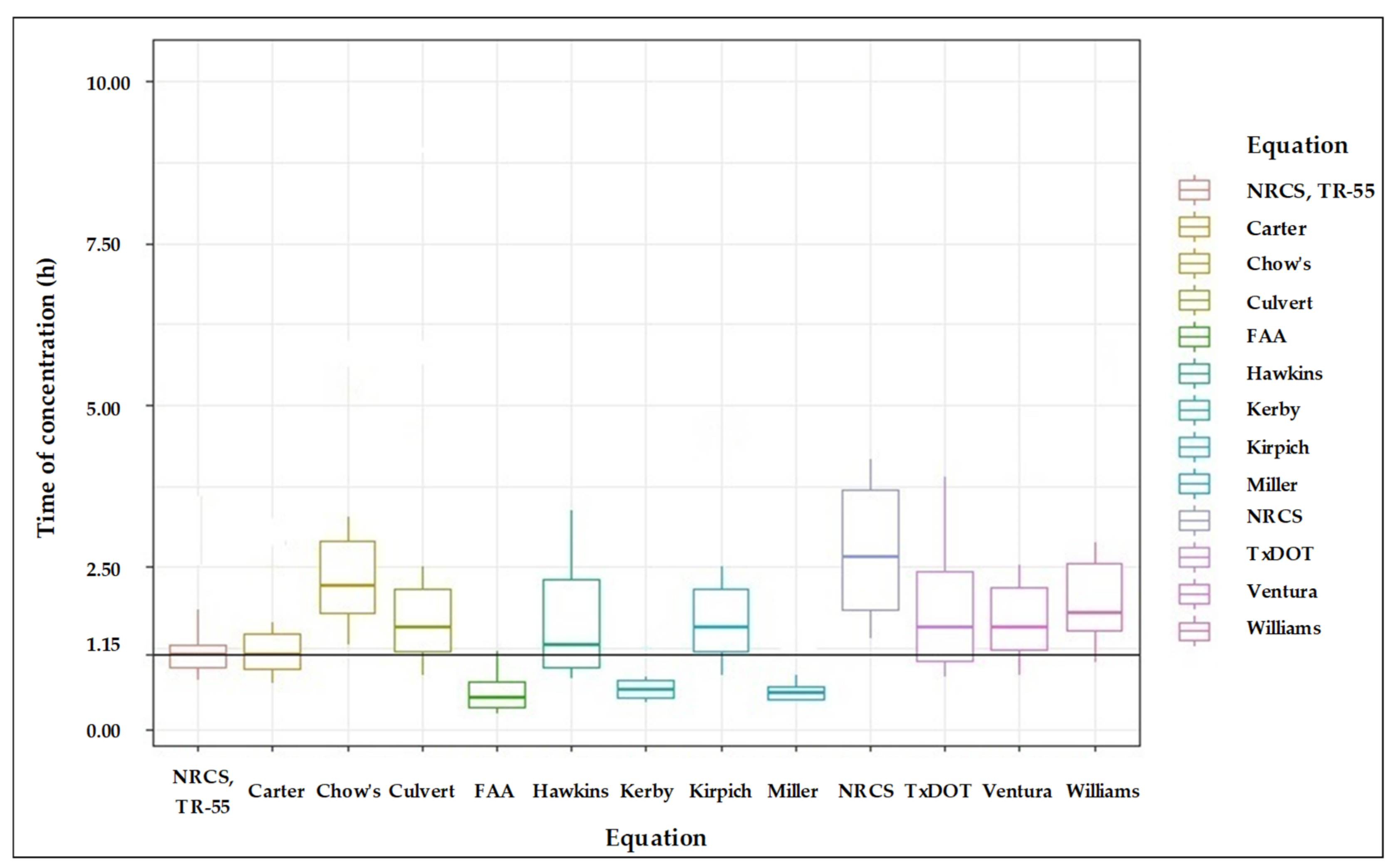
To estimate the time of concentration of the different selected water basins, in this study 12 empirical equations were used, the resulting values of which are displayed in Table 4. In effect, it was found that there were significant differences in the calculated Tc values when the results of each equation are compared for each studied basin. In this regard, Vélez and Gutiérrez (2011) [3] consider that it is appropriate to use a large number of equations to calculate the time of concentration in order to reduce the level of uncertainty of the calculated data, and to discard the equations that are outside the range. Due to the above, it is of great value to have a significant number of empirical equations to calculate the time of concentration in a specific region, because it creates a range of alternatives that can be assessed by the researchers in terms of the results obtained, and enables the use of statistical comparison methods to filter and reduce the number of initial equations to a small number that according to the comparison test provides similar values for the calculation of Tc.

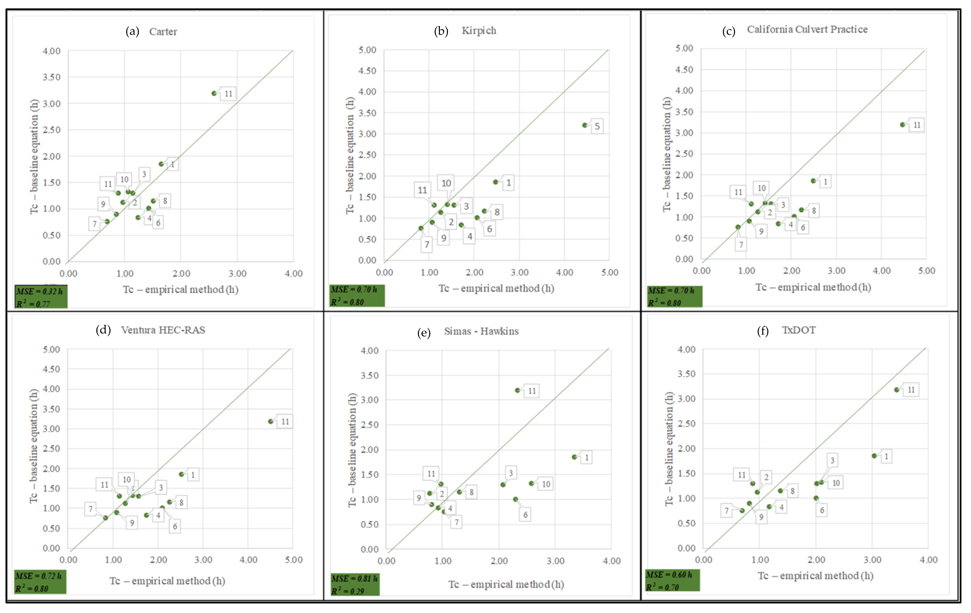
When the method for estimating Tc is categorized by means of statistical analysis (ANOVA), Dunn’s means comparison test, and the calculation of R² and MSE, the results of the formal hypothesis test of the Tc (treatments), Fo = 17.15, yielded a p value < 0.0001, and additional hypothesis testing was performed for the micro-basins (blocks), Fo = 23.26, with a p value < 0.0001. The results obtained in the comparison test are displayed in Table 6, and Table 7 displays the goodness of fit results. These results lead to the belief that of the 12 empirical equations selected, 6 did not display significant differences when the mean values are compared to those of the baseline equation, among which the Carter equation was the equation with the best goodness of fit according to the selection criteria that were adopted. However, the results of the other equations cannot be ruled out because the decision criteria are not rejected for these cases either. The results of the means comparison test can be compared to those obtained by Vahabzadeh, G., Saleh, I., Safari, A., & Khosravi, K. (2013) [2], who used the Tukey means comparison test to categorize the best equations. Additionally, the comparison criteria used in this study are supported by Ravazzani, G., Boscarello, L., Cislaghi, A., & Mancini, M. (2019) [19], who based their goodness of fit of the methods on MSE and R². On the above, it is important to mention that the use of a means comparison test plays an important role in the categorization of the equations of the study, as it enables the researcher the rule out many of the equations that were initially selected that do meet the expected objectives. Afterwards, assessing which of the resulting methods is most accurate compared to the baseline equation brings the researcher closer to the desired objective, providing backing for the methodological approach and validation that an empirical equation may be highly correlated with an equation almost fully based on physics. Lastly, it can be said that these statistical methods leave a window open to study the remaining equations from a different perspective (sensitivity analysis). The curve number was estimated for each urbanized watershed and extreme scenarios of antecedent moisture conditions were considered [33].

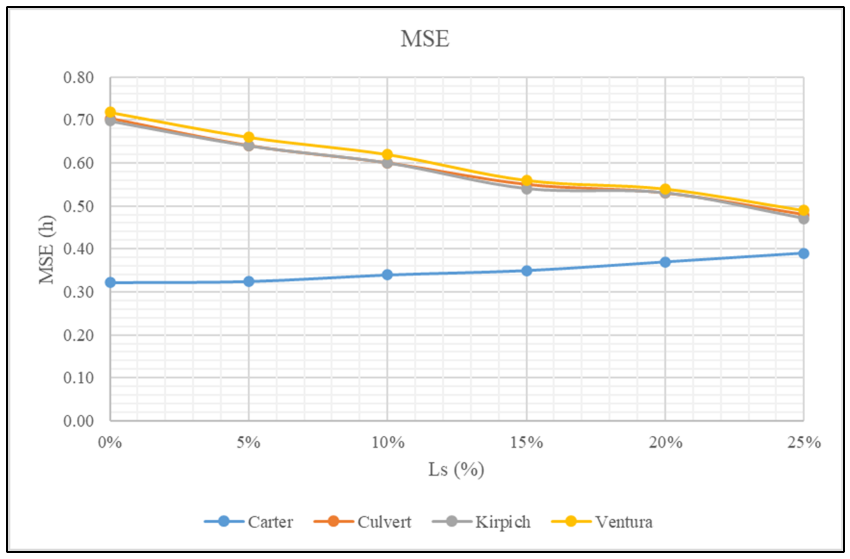
For the effects of sensitivity analysis, changes were made to the magnitudes of some parameters for the calculation of the time of concentration of the selected equations. Four sensitivity analyses were conducted with the results displayed in Table 8, Table 9 and Table 10 and Figure 7 and Figure 8. These results show that by changing the magnitude of the sensitized parameters, in some cases no sensitivity was observed, as in the case of changing the sheet flow travel time. In other cases, the precision of the statistical analysis (MSE) was negatively affected, as when the travel times of the baseline equation were discriminated. Lastly, in some empirical equations (Kirpich and TxDOT), the difference compared to the NRCS equation decreased when lengths and ground cover were changed. These results can be compared with those of the study by Michailidi, E.M., Antoniadi, S., Koukouvinos, A., & Bacchi, B. &. (2018) [34], who performed sensitivity analysis with changes in the discretization of the accumulation of the flow and changed the roughness coefficient. In analyzing these results, it can be inferred that in some equations, when the magnitude of parameters is adequately changed, efficient results are obtained, which may represent an alternative for the effects of calculating Tc. In this way, the researcher is not limited to solely approaching the calculation of the runoff flow rate using the Carter equation in this case. Instead, there are other alternatives available as demonstrated in this study. They could be useful for verifying the Tc value by means of alternative and reliable equations, thus increasing the reliability of the process of calculating the flow rate using rainfall-runoff models. The sensitivity analysis was only conducted for urban catchments considering similar empirical equations used by other authors [35].

6. Conclusions

The rigorous approach of this research study is evident in the methodology presented for its performance. The delimitation of the urban watersheds is the starting point for a series of processes that must be conducted in order to estimate the time of concentration, such as the identification of the morphometric and geometric parameters of the main watercourses of the basins of the study. The information required for this research study on the aforementioned parameters was obtained from drawings with topographic information and field measurements made with high-precision topographic equipment. This equipment was used to perform plan and altitude surveys using conventional methodologies of direct measurement with electronic total station and indirect measurements using RTK GPS technology.

The equation proposed by the NRCS was used as reference (or baseline formulation) to determine the time of concentration of basins under general conditions, and for this reason, whenever possible, this method should be the first choice for calculating Tc. However, when there is not sufficient information available to calculate Tc using the baseline equation, or depending on the stage of phase of the project to be implemented (pre-feasibility or feasibility), empirical equations that do not display significant differences may be used.

The most effective method for estimating the time of concentration of the urban watersheds of the city of Montería is the Carter equation based on Mean Square Error (MSE) and Coefficient of Determination (R²). These values were found taking into consideration the total length of the main watercourse using the Carter equation, which is equivalent to the sum of the different travel times of the baseline equation using laminar, concentrate, and channel flow. Complementarily, it can be concluded that the Carter equation was found to have highly significant similarity with the baseline equation for the effects of calculating the Tc, which is validated by the value found in the means in the statistical analysis, in which values were reported of 1.34 h for the baseline equation and 1.28 h for the Carter equation (see Figure 5).

The comparison of the baseline equation to the empirical methods that estimate Tc enabled showing the correlations between them. However, statistical analysis is the best way to select the adjustment method that demonstrates the relevance of the model for a particular basin. In this study, statistical analysis enabled the disaggregation of the components used in engineering to calculate the Tc of a basin. Thanks to the analysis of variance, the significant differences between the times of concentration of the proposed equations steered the study towards application of Dunnet’s comparison of means test, which helped select the set of equations that, in this case, best fit the requirements of the urban watersheds of the city of Montería, Córdoba.

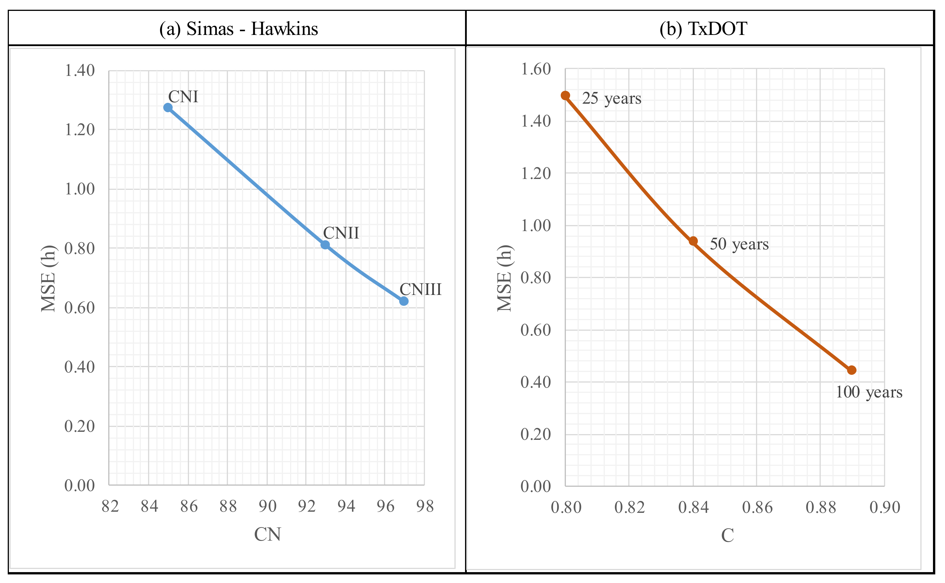
By means of sensitivity analysis it was shown that the results of the equations with best goodness of fit according to the statistical analysis were those by Kirpich, California Culvert Practice and Ventura, which were the equations that displayed sensitivity to the length of the main watercourse (Ls). As Ls decreased, MSE decreased, and a 25% reduction was the largest reduction of Ls at which the MSE stabilized. The ground cover and texture were found to be highly sensitive variables when the Simas-Hawkins equation is used, which is a function of the curve number, and the TxDOT, as a function of the runoff coefficient. It can be concluded that for the first equation mentioned here, MSE decreased considerably when background conditions of moisture were considered (AMC III), with MSE of 0.62 h. In the second equation mentioned in this point, it is concluded that as the value of the runoff coefficient (C) increases as a function of the return period, MSE decreases, with a result of 0.44 h for a 100-year Tr.

For future works, the use of data in monitored basins should be utilized to measure the time concentration (time between rain end and superficial flow end) for comparing these values with the NRCS equation (baseline formulation) and the twelve empirical equations.

References

1. González-Álvarez, Á.; Viloria-Marimón, O.M.; Coronado-Hernández, Ó.E.; Vélez-Pereira, A.M.; Tesfagiorgis, K.; Coronado-Hernández, J.R. Isohyetal maps of daily maximum rainfall for different return periods for the Colombian Caribbean Region. Water 2019, 11, 358. [Google Scholar] [CrossRef]
2. Vahabzadeh, G.; Saleh, I.; Safari, A.; Khosravi, K.; Vahabzadeh, G.; Saleh, I.; Safari, A.; Khosravi, K. Determination of the best method of estimating the time of concentration in pasture watersheds (case study: Banadak Sadat and Siazakh Watersheds, Iran). J. Biodivers. Environ. Sci. 2013, 3, 150–159. [Google Scholar]
3. Vélez, J.J.; Gutierrez, B.A. Estimación del tiempo de concentración y tiempo de rezago en la cuenca experimental urbana de la quebrada San Luis, Manizales. Dyna 2011, 78, 58–71. [Google Scholar]
4. Avila, L.; Ávila, H. Hazard Analysis in Urban Streets Due to Flash Floods: Case Study of Barranquilla, Colombia. In World Environmental and Water Resources Congress; American Society of Civil Engineers: Reston, VA, USA, 2016; pp. 144–154. Available online: ascelibrary.org (accessed on 9 September 2021).
5. Salimi, E.T.; Nohegar, A.; Malekian, A.; Hoseini, M.; Holisaz, A. Estimating time of concentration in large watersheds. Paddy Water Environ. 2017, 15, 123–132. [Google Scholar] [CrossRef]
6. McCuen, R.H.; Wong, S.L.; Rawls, W.J. Estimating urban time of concentration. J. Hydraul. Eng. 1984, 110, 887–904. [Google Scholar] [CrossRef]
7. Amatya, D.; Cupak, A.; Walega, A. Influence of tIme of concentratIon on variation of runoff from a small urbanized watershed. Geomat. Landmanagement Landsc. 2015, 2, 7–19. [Google Scholar]
8. Ibáñez, S.A.; Moreno, H.R.; Gisbert, J.M.B. Métodos Para la Determinación del Tiempo de Concentración (tc) de una Cuenca Hidrográfica; Universidad Politecnica de Valencia: Valencia, Spain, 2011. [Google Scholar]
9. Grimaldi, S.; Petroselli, A.; Tauro, F.; Porfiri, M. Time of concentration: A paradox in modern hydrology. Hydrol. Sci. J. 2012, 57, 217–228. [Google Scholar] [CrossRef]
10. Fang, X.; Thompson, D.B.; Cleveland, T.G.; Pradhan, P. Variations of Time of Concentration Estimates Using NRCS Velocity Method. J. Irrig. Drain. Eng. 2007, 133, 314–322. [Google Scholar] [CrossRef]
11. De Almeida, I.K.; Almeida, A.K.; Anache, J.A.A.; Steffen, J.L.; Alves, T. Estimation on time of concentration of overland flow in watersheds: A review. Geociências 2014, 33, 661–671. [Google Scholar]
12. Gericke, O.J.; Smithers, J.C. Review of methods used to estimate catchment response time for the purpose of peak discharge estimation. Hydrol. Sci. J. 2014, 59, 1935–1971. [Google Scholar] [CrossRef]
13. Sharifi, S.; Hosseini, S.M. Methodology for Identifying the Best Equations for Estimating the Time of Concentration of Watersheds in a Particular Region. J. Irrig. Drain. Eng. 2011, 137, 712–719. [Google Scholar] [CrossRef]
14. U.S. Department of Agriculture Natural Resources Conservation Service (USDA-NRSC); C.E.D. Urban Hydrology for Small Watersheds, Technical Release 55 (TR-55); U.S. Department of Agriculture Natural Resources Conservation Service (USDA-NRSC), C.E.D.: Washington, DC, USA, 1986.
15. Kirpich, Z.P. Time of concentration of small agricultural watersheds. Civ. Eng. 1940, 10, 362. [Google Scholar]
16. Gericke, O.J.; Smithers, J.C. Are estimates of catchment response time inconsistent as used in current flood hydrology practice in South Africa? J. S. Afr. Inst. Civ. Eng. 2016, 58, 2–15. [Google Scholar] [CrossRef]
17. Miller, W. Evolving a shortcut for design of storm sewers. Munic 1951, 89, 42–59. [Google Scholar]
18. Highways, C.D.O. California Culvert Practice; Department of Public Works, Division of Highways: Sacramento, CA, USA, 1960.
19. Ravazzani, G.; Boscarello, L.; Cislaghi, A.; Mancini, M. Review of Time-of-Concentration Equations and a New Proposal in Italy. J. Hydrol. Eng. 2019, 24, 04019039. [Google Scholar] [CrossRef]
20. Carter, R.W. Magnitude and Frequency of Floods in Suburban Areas; U.S. Geological Survey: Reston, VA, USA, 1961.
21. Federal Aviation Agency (FAA). Airport Drainage; Department of Transport Advisory Circular: Washington, DC, USA, 1970.
22. Welle, P.I.; Woodward, D. Engineering Hydrology—Time of Concentration; Bloomsbury Publishing: London, UK, 1986. [Google Scholar]
23. Texas Department of Transportation. Hydraulic Design Manual (Revised); Texas Department of Transportation: Austin, TX, USA, 1994.
24. Li, M.-H.; Chibber, P. Overland Flow Time of Concentration on Very Flat Terrains. Transp. Res. Rec. J. Transp. Res. Board 2008, 2060, 133–140. [Google Scholar] [CrossRef] [Green Version]
25. Li, M.-H.; Chibber, P.; Cahill, A.T. Estimating time of concentration of overland flow on very flat terrains. In 2005 ASAE Annual Meeting; American Society of Agricultural and Biological Engineers: St. Joseph, MI, USA, 2005; p. 1. [Google Scholar]
26. Chow, T.; Maidment, D.; Mays, L. Applied Hydrology; McGraw-Hill: New York, NY, USA, 1988. [Google Scholar]
27. Williams, G. Flood discharges and the dimensions of spillways in India. Engineering 1922, 134, 321–322. [Google Scholar]
28. Fang, X.; Thompson, D.B.; Cleveland, T.G.; Pradhan, P.; Malla, R. Time of concentration estimated using watershed parameters determined by automated and manual methods. J. Irrig. Drain. Eng. 2008, 134, 202–211. [Google Scholar] [CrossRef]
29. Kerby, W.S. Time of concentration for overland flow. Civ. Eng. 1959, 29, 60. [Google Scholar]
30. González, Á.; Molina, J.; Meza, B.; Viloria, O.; Tesfagiorgis, K.; Mouthón, J. Assessing the Performance of Different Time of Concentration Equations in Urban Ungauged Watersheds: Case Study of Cartagena de Indias, Colombia. Hydrology 2020, 7, 47. [Google Scholar] [CrossRef]
31. Coronado-Hernández, Ó.E.; Merlano-Sabalza, E.; Díaz-Vergara, Z.; Coronado-Hernández, J.R. Selection of Hydrological Probability Distributions for Extreme Rainfall Events in the Regions of Colombia. Water 2020, 12, 1397. [Google Scholar] [CrossRef]
32. Kobiyama, M.; Grison, F.; Lino, J.F.L.; Silva, R.V. Time of concentration in the UFSC campus catchment, Florianópolis-SC (Brazil), calculated with morfometric and hydrological methods. In Proceedings of the Regional Conference on Geomorphology, UFG-IUG, Goiania, Brazil, 6–10 September 2006; Volume 110. [Google Scholar]
33. Krisnayanti, D.; Bunganaen, W.; Frans, J.H.; Serán, Y.; Legono, D. Curve Number Estimation for Ungauged Watershed in Semi-Arid Region. Civ. Eng. J. 2021, 7, 1070–1083. [Google Scholar] [CrossRef]
34. Michailidi, E.M.; Antoniadi, S.; Koukouvinos, A.; Bacchi, B.; Efstratiadis, A. Timing the time of concentration: Shedding light on a paradox. Hydrol. Sci. J. 2018, 63, 721–740. [Google Scholar] [CrossRef] [Green Version]
35. Lopes, A.L. Performance of time of concentration formulas for urban and rural basins. Rev. Bras. Recur. Hídricos 2005, 10, 5–23. [Google Scholar]
Figure 1. Illustration drawing of the three time of concentration flows of the equation proposed by the NRCS.
Water 14 02847 g001
Figure 2. Identification of concentrated flow and channel flow in one of the small watersheds of the case study (city of Montería, Colombia).
Water 14 02847 g002
Figure 3. Geographic location of the municipality of Montería.
Water 14 02847 g003
Figure 4. Selected small urban watersheds and main watercourses.
Water 14 02847 g004
Figure 6. Tc graphs estimated with empirical methods versus Tc calculated with the baseline equation: (a) Carter; (b) Kirpich; (c) California Culvert Practice; (d) Ventura; (e) Simas-Hawkins; and (f) TxDOT.
Water 14 02847 g006
Figure 7. Calculation of MSE changing Ls.
Water 14 02847 g007
Figure 8. Calculation of MSE changing CN and C: (a) Simas-Hawkins; and (b) TxDOT.
Water 14 02847 g008