
Optimal Sprinkler Application Rate of Water–Fertilizer Integration Machines Based on Radial Basis Function Neural Network

1
School of Mechanical and Electrical Engineering, Guangzhou University, Guangzhou 510006, China
2
Guangdong Engineering Research Centre for High Efficient Utility of Water, Fertilizers and Solar Intelligent Irrigation, Guangzhou University, Guangzhou 510006, China
3
Advanced Institute of Engineering Science for Intelligent Manufacturing, Guangzhou University, Guangzhou 510006, China
*
Author to whom correspondence should be addressed.
Water 2022, 14(18), 2838; https://doi.org/10.3390/w14182838
Submission received: 20 August 2022
/
Revised: 6 September 2022
/
Accepted: 7 September 2022
/
Published: 12 September 2022
(This article belongs to the Special Issue Advances in Sprinkler Irrigation Systems and Water Saving)
Abstract
:The application rate for sprinkler irrigation of water–fertilizer integration machines is an important technical parameter for efficient operation. If the value is too large, the equipment will produce runoff; if it is too small, the equipment will run too long and waste energy. Therefore, it is necessary to provide a feasible scientific and theoretical basis for developing a reasonable application rate. In this study, a mathematical model of soil infiltration for sprinkler irrigation with water and fertilizer integration machines was developed. Soil water accumulation time for different soil’s initial water content, bulk density, sprinkler application rate and soil texture were derived by the finite element method, and these data were used as a training database for the neural network. To make the neural network convenient for predicting the optimal application rate of sprinkler irrigation (the maximum application rate of sprinkler irrigation without runoff) in practice, the time of waterlogging, was multiplied by the optimal application rate of sprinkler irrigation to obtain the total irrigation volume. The optimal application rate of the sprinkler irrigation prediction model of radial basis function (RBF) neural network was constructed with total irrigation water, soil bulk density, initial water content and soil texture as inputs and compared with BP neural network and generalized regression neural network. The highest prediction accuracy of RBF neural network was obtained, and its average relative error was 0.11. To verify the accuracy of the RBF neural network application rate of sprinkler irrigation prediction model in real life, a sprinkler experiment was conducted in the laboratory of Guangzhou University, and the collected soil and lawn of Guangzhou University were used to simulate the actual environment. The results showed that the relative error between the RBF neural network prediction results and the actual values was generally around 10%, while for a total irrigation volume of 58 mm, the optimal application rate of sprinkler irrigation calculated with the model was 42 (mm/h), which can save 70% of irrigation time compared to the case of using the stable infiltration rate of soil as the application rate of sprinkler irrigation without water and fertilizer. Water and fertilizer losses were not observed. This indicates that the model proposed in this study is of practical value in determining the optimum application rate of sprinkler irrigation for water–fertilizer integration machines.
1. Introduction
Agriculture irrigation accounts for 70% of water use worldwide and over 40% in many OECD countries. Thus, improving the efficiency of agricultural water use is a matter of national importance. Sprinkler irrigation technology saves water, labor, and increases production, therefore, it is strongly promoted by many countries. As an important parameter of sprinkler irrigation technology, the application rate plays a pivotal role in the efficient operation of sprinkler irrigation equipment. When the application rate of the sprinkler irrigation is too high, it can lead to runoff. When the application rate of the sprinkler irrigation is too low, it can result in inefficient operation. This will result in increased operating and maintenance costs. Therefore, it is of great economic and social significance to study the optimum application rate [1,2,3].
The application rate of sprinkler irrigation is selected in two ways. The first is to select the application rate that is not greater than the stable infiltration rate of the soil. James et al. [4] presented that the application rate is mostly selected in this manner. When stable infiltration rate is used, the sprinkler does not produce runoff. The second approach is to use a sprinkler application rate that is greater than the steady infiltration rate. Gencoglan et al. [5] prevented soil runoff by intermittent irrigation when using high sprinkler intensities. The intermittent period is determined by the time of water accumulation according to the Horton and Kostiakov equation. Espinosa et al. [6] obtained the maximum application rate of sprinkler irrigation without runoff and the maximum allowable sprinkler rate for different combinations of slope and soil type on agricultural fields with slopes between 16 and 30% through experiments, and verified its feasibility on slopes with a 16% slope. Dadhich et al. [7] established a mathematical equation of soil infiltration rate and sprinkler irrigation application rate. The sprinkler irrigation time was lowest and the efficiency was greatly improved by varying application rate of sprinkler irrigation. DeBoer et al. [8] proposed that the previous application rate of sprinkler irrigation was estimated based on a mathematical model of a single soil infiltration relationship, which was less accurate and soil infiltration was affected by multiple parameters. The results of experiments in the field showed that the value of soil hydraulic conductivity parameter increased with the increase of the application rate of sprinkler irrigation. Therefore, the appropriate parameter values for the Green and Ampt equation are specific to the application rate of sprinkler irrigation, and the prediction results will be very different if the parameter values are not selected properly. The above studies are important guidelines for developing optimal sprinkler application rates. However, due to the large number of parameters affecting the rates, when some of these parameters were used to build prediction models, the prediction errors of the models were large. In addition, due to the complexity of soil infiltration experimental operations, less data is available. In recent years, more and more computer intelligence algorithms have been used in the field of irrigation. Some examples are ant colony algorithms, genetic algorithms, deep learning, artificial neural networks and fuzzy prediction [9,10,11]. Many of these show great potential for application in the field of efficient irrigation. Therefore, the use of neural network models to predict optimal sprinkler rate has very important practical applications.
Gu et al. [12] proposed an improved BP neural network algorithm that can represent maize yield under different irrigation systems. Chen et al. [13] developed a water demand prediction model for greenhouse tomatoes using an improved T-S fuzzy neural network. Al-Naji et al. [14] proposed to obtain soil characteristics through computer vision, and then input these characteristics into the neural network to predict whether the soil needs to be irrigated. The system they propose is simple, inexpensive, and a promising technology. The soil moisture required for irrigation varies widely and, based on farmers’ experience alone, may result in imprecise irrigation. Perea et al. [15] developed a hybrid approach combining artificial neural networks, fuzzy logic, and genetic algorithms for irrigation depth prediction. This method has been tested in real life with good results.
The purpose of this paper is to study the parameters affecting the soil water accumulation time by establishing a model of soil infiltration during sprinkler irrigation and obtaining a large amount of neural network training data through finite elements. At the same time, the prediction model of the optimal application rate of sprinkler irrigation (the maximum application rate of sprinkler irrigation without runoff) is obtained by a neural network and applied to real life to improve the efficiency of runoff-free sprinkler irrigation by water and fertilizer integration machine. In this way, the operating cost and maintenance cost of the equipment can be reduced. In Section 2, we focus on modeling the soil infiltration during sprinkler irrigation and apply the finite element method to obtain the dataset required for neural network training. In Section 3, the structure of the input and output layers of the neural network is given as a six-input single-output structure. In Section 4, preprocessing of the data to be trained to reduce the effect of different units of data on the convergence of neural network is discussed. In Section 5, we introduce the theory of three neural networks. In Section 6, the evaluation method of the training accuracy of the neural networks is presented. In Section 7 the prediction results of the three neural networks are compared. The empirical formula for the total soil water requirement is given in Section 8, and the feasibility of the neural network predictions is verified experimentally in Section 9. The advantages of using the optimal sprinkler application rate over the conventional sprinkler application rate in terms of efficiency and energy reduction in irrigating lawns are demonstrated in Section 10.
2. Neural Network Training Set Data Acquisition
2.1. RBF Neural Network Basic Theory
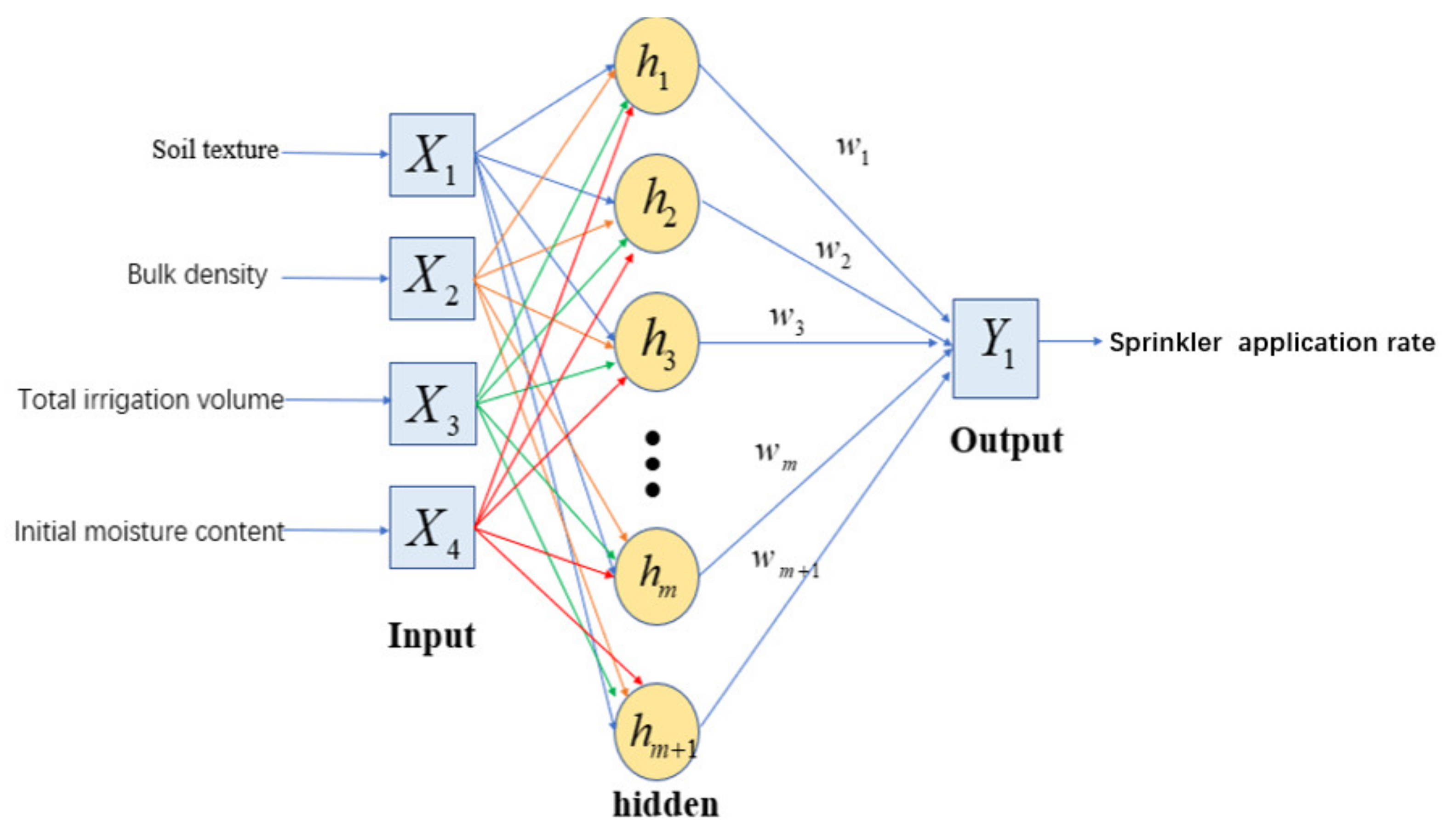
Radial basis function (RBF) neural network is a three-layer forward neural network with hidden layers. It transforms the low-dimensional input data into the high-dimensional space by the radial basis function of the hidden layer, so that the linearly indistinguishable data in the low-dimensional space is linearly distinguishable in the high-dimensional space [16]. As shown in Figure 1, the boxes inside are the inputs and outputs, and the circles inside are the neurons. The h in the figure is the radial basis function, which is a nonlinear mapping from the input layer to the hidden layer through which the data that is not separable in the low dimension is mapped to the high dimension by the radial basis containing a function to make it separable. From the hidden layer to the output layer is a linear combinatorial relationship that segments the high-dimensional separable data by selecting appropriate weights w. The radial basis function of RBF neural networks generally uses a Gaussian function of the following form [17].
is the center of the radial basis function, is the width parameter, which controls the radial range of action of the function.
The linear output equation of RBF is shown below.
Bring Equation (10) into Equation (11) to get the input and output relationship equation.
2.2. Spray Irrigation Soil Hydrology Model
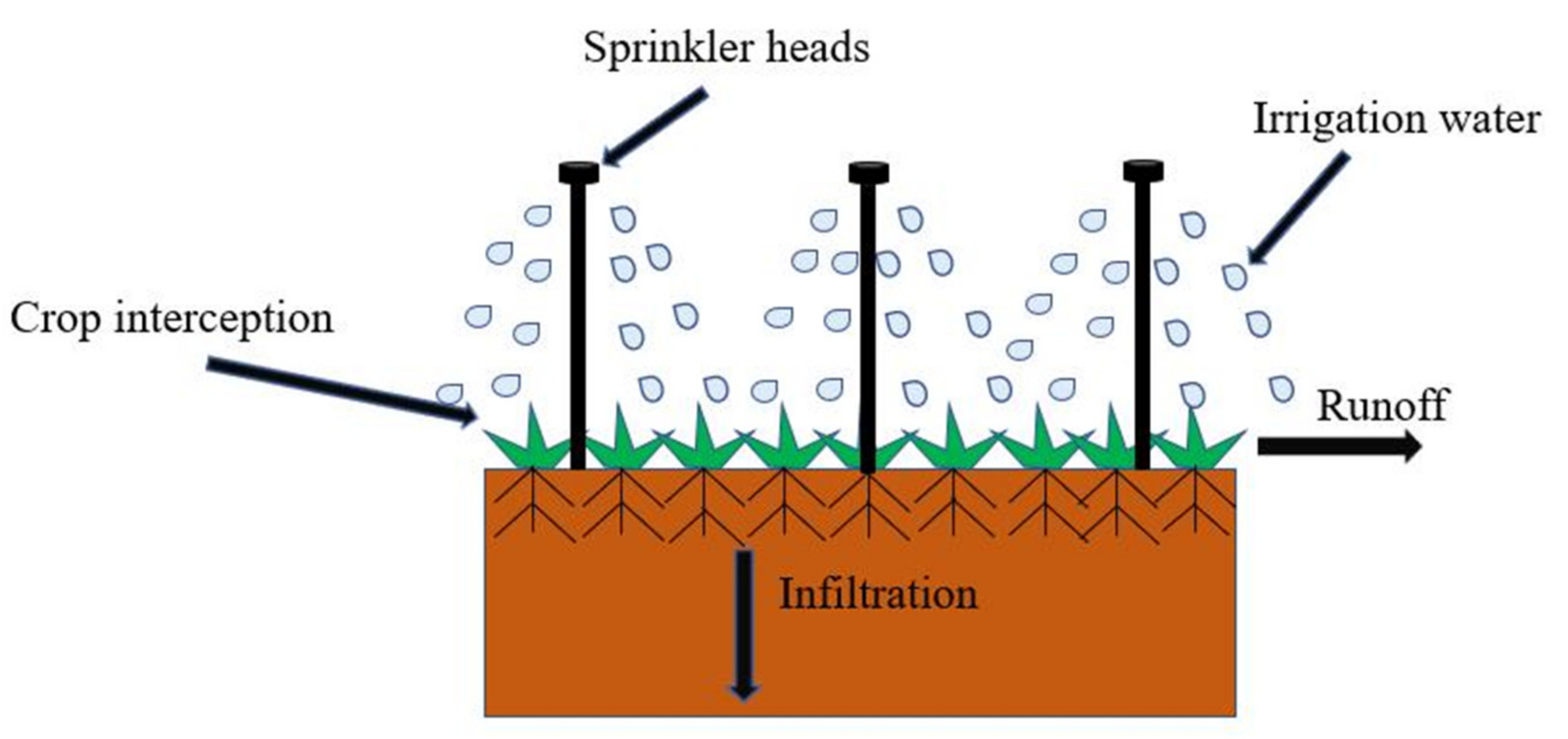
The form of irrigation water conversion during sprinkler irrigation is shown in Figure 2. When irrigation water exits the sprinkler head, part of the water infiltrates into the soil, part of it is intercepted by crop leaves and branches, and part of the water cannot infiltrate the soil surface due to saturation and disburses as runoff. Under sprinkler irrigation conditions, the infiltration process of the soil is a one-dimensional vertical infiltration process, which can be described by the one-dimensional Richards.
2.2.1. Soil Water Infiltration Process Equation
The infiltration movement of unsaturated soil water is mainly driven by its gravitational and matrix potentials (). The unsaturated soil water flux can be found by bringing it into Darcy’s law.
where is the soil water flux and is the unsaturated hydraulic conductivity.
The unsaturated soil water movement follows not only Darcy’s law but also the continuity principle of mass conservation. The Richards equation revealing the variation of moisture content () in soil with time can be derived from Darcy’s law and the continuity equation [18].
2.2.2. Unsaturated Soil Hydraulic Properties Function
To solve the numerical solution of Richards’ formula, the soil moisture characteristic curve and unsaturated hydraulic conductivity were depicted by the empirical formula van Genuchten model [19,20].
where and are the residual water content and saturation water content, respectively. is the effective saturation, which is used to reflect the extent to which the soil pores are filled with water. When is equal to 0, it means that the water content of the soil is equal to the residual water content, and the soil is completely dry at this time. When is equal to 1, it means that the water content of the soil is equal to the saturation water content, and the soil is in a saturated state at this time. is the saturated hydraulic conductivity, which is significantly influenced by the pore state of the soil. , , and are empirical parameters that express the properties of the soil.
2.2.3. Irrigation Water Interception Equation
Irrigation interception is the amount of irrigation water falling from sprinkler irrigation that is intercepted by the foliage and branches of the crop. The formula is shown below [21].
where is the amount of irrigation water intercepted by the crop, is the irrigation intensity of the crop, and a and b are empirical constants for the crop. For most crops, a is 0.25 and b is approximately equal to the soil cover fraction (SCF). is the leaf area index.
Leaf area index is the ratio of the projected area of crop leaves on the soil to the land area. It is an important indicator of crop planting structure, the larger the leaf area index the greater the crop’s effect on irrigation water retention, but also affects the normal respiration of the crop. The calculation formula is shown below:
where and are the length and width of the measured crop leaves, respectively. n is the total number of leaves of the ith crop, m is the number of measured crops, and is the density of the planted crops.
Soil cover fraction can be calculated by the following equation:
where K is the extinction coefficient, which is generally between 0.5 and 0.75 for most cases. The extinction coefficient used in this paper is taken as 0.6.
2.2.4. Soil Profile Parameter Setting
The initial state of the soil during sprinkler irrigation is given by the following equation:
is the state of water content of each layer of the soil at the initial moment. is the height of the experimental soil column.
In the sprinkler process, we choose to use the free drainage boundary for the lower boundary and the atmospheric boundary for the upper boundary, which can be expressed by the following equation.
When the irrigation time is less than the waterlogging time (), the infiltration flux of the soil is equal to the applied application rate of sprinkler irrigation ; when the sprinkler time is greater than the waterlogging time the surface of the soil appears waterlogged, is the thickness of the waterlogged soil surface.
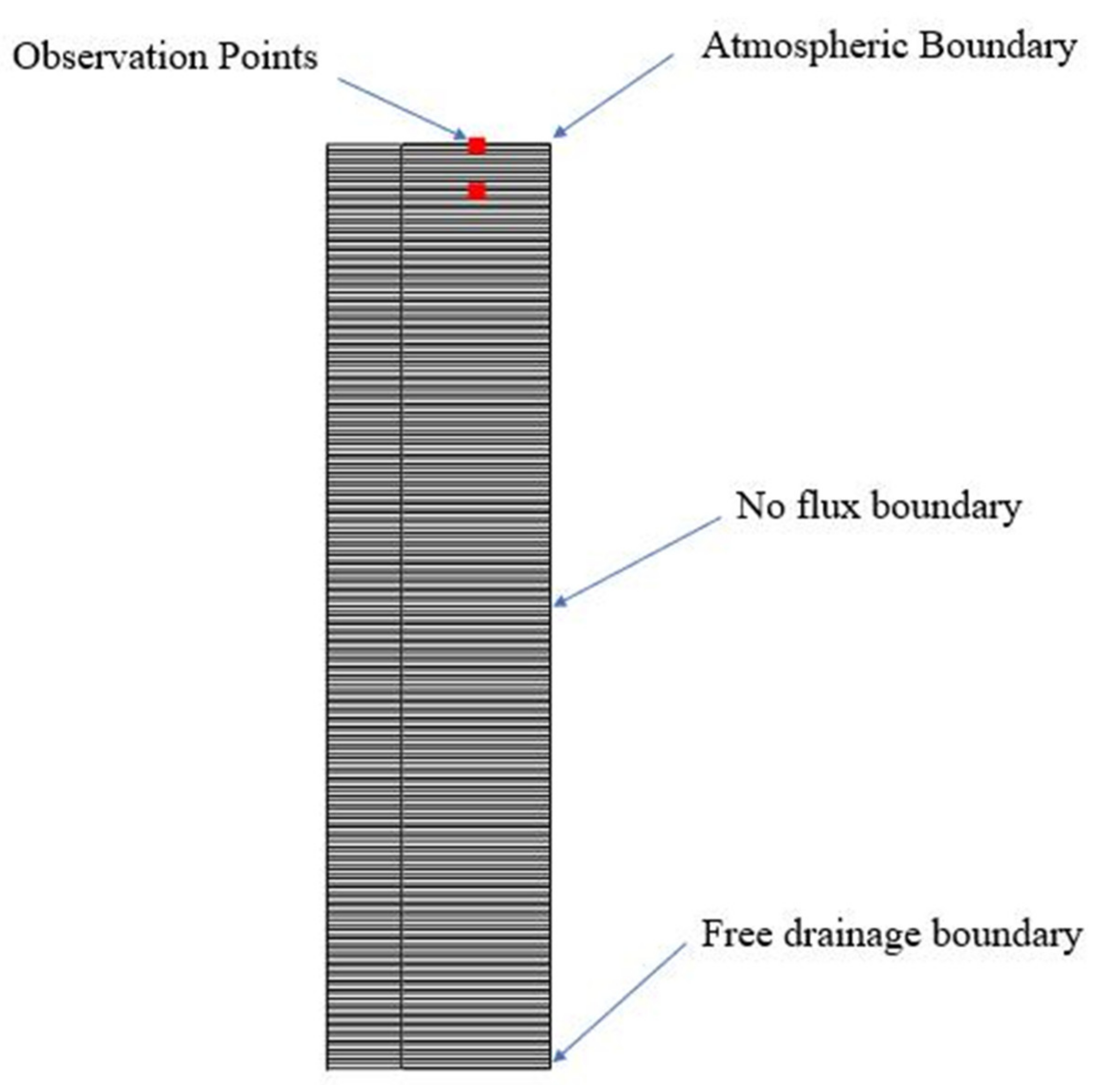
The finite element division of the soil profile is shown in Figure 3. The finer the division, the higher the accuracy of the finite element calculation, but the amount of computation increases. Moreover, observation points are set up on the soil profile to record when water accumulation occurs in the soil.
2.3. Determination of Simulation Parameters
Since Guangdong belongs to the eastern coastal region and has a large number of sandy loam soils, this paper focuses on the infiltration performance of sprinkler irrigation in sandy loam soils with different compositions. As shown in Table 1, seven different groups of sandy loam soils were selected for simulation experiments.
In the field experiment, the initial moisture of the soil generally varies from 6% to 20% [22], so the initial moisture as shown in Table 2 was selected as a simulation parameter in this paper. The bulk density of sandy soils generally ranges between 1.1 g/cm3 and 1.5 g/cm3. Therefore, in this paper, four parameters are selected from this interval and used as simulation parameters.
2.4. Acquire and Analyze Data
2.4.1. Simulation Data
Seven different soil types, eight different initial water contents and sprinkler application rate, and four different soil bulk density were simulated after permutation and combination, and the cases of no standing water and sufficient water supply were excluded. Finally, 1376 sets of data were obtained. Some of the data are presented in Table 3.
2.4.2. Data Analysis
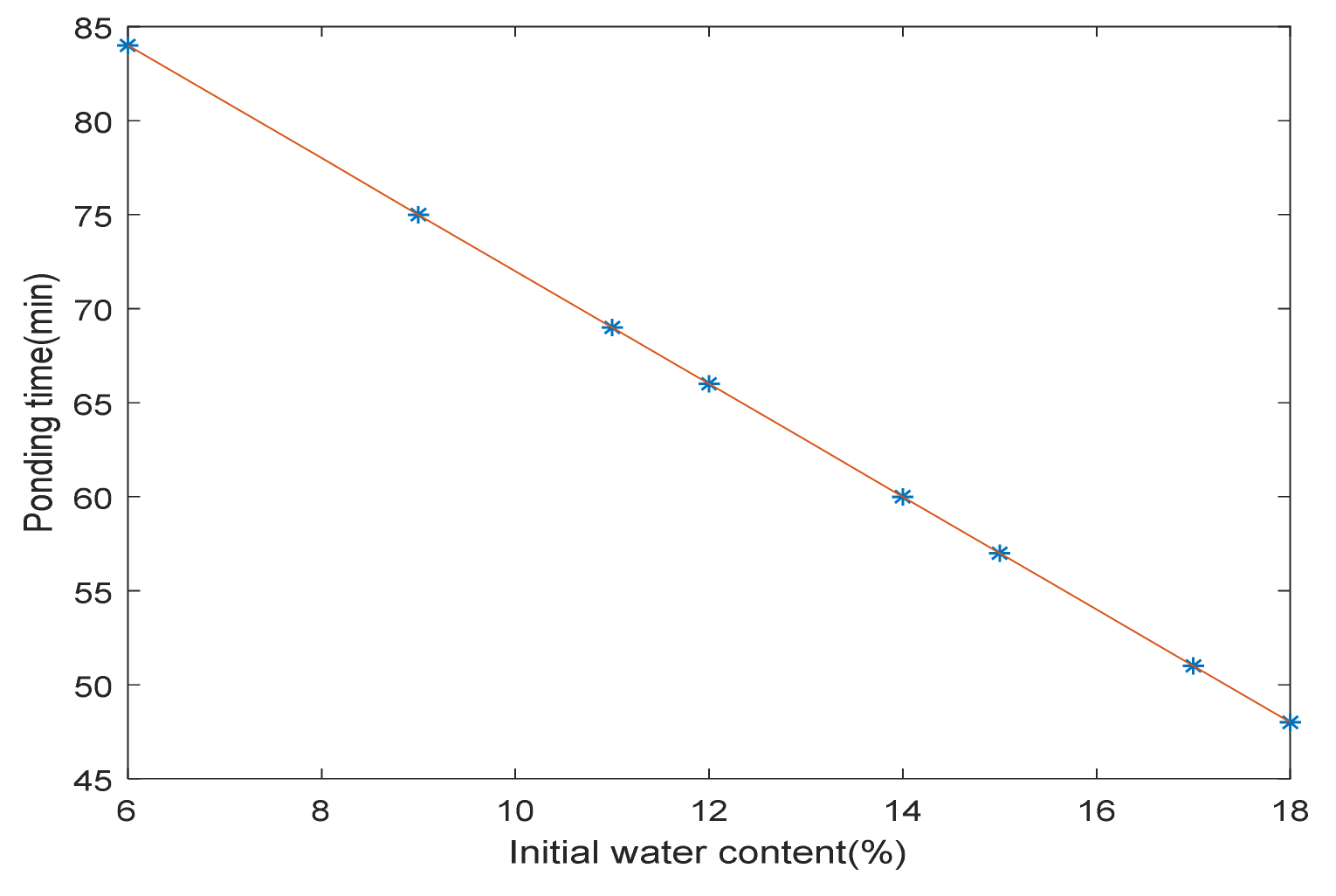
As shown in Figure 4, when the soil texture, application rate of sprinkler irrigation, and bulk density are the same, the waterlogging time of the soil decreases as the initial soil moisture content increases, and their relationship is approximately linear. The larger the initial water content of the soil, the smaller the water potential gradient of the soil, and the smaller the driving force of soil water infiltration. Therefore, the ability of water infiltration of sprinkler irrigation falling on the soil surface decreases with the increase of the initial water content of the soil, and the soil is more likely to produce water ponding.
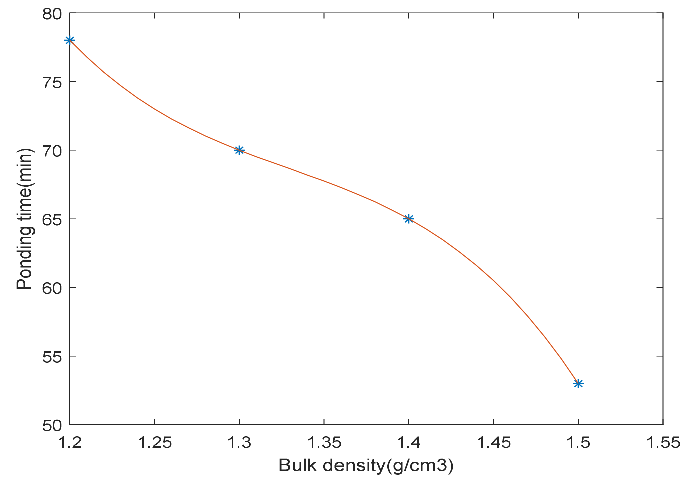
As shown in Figure 5, with the same application rate of sprinkler irrigation, soil texture, and initial water content, the waterlogging time of the soil decreases with increasing soil bulk density. The greater the bulk density of the soil, the more compacted the soil, the smaller the pore space in the soil, the greater the ability to block the infiltration of soil water, the soil is more likely to produce accumulated water.
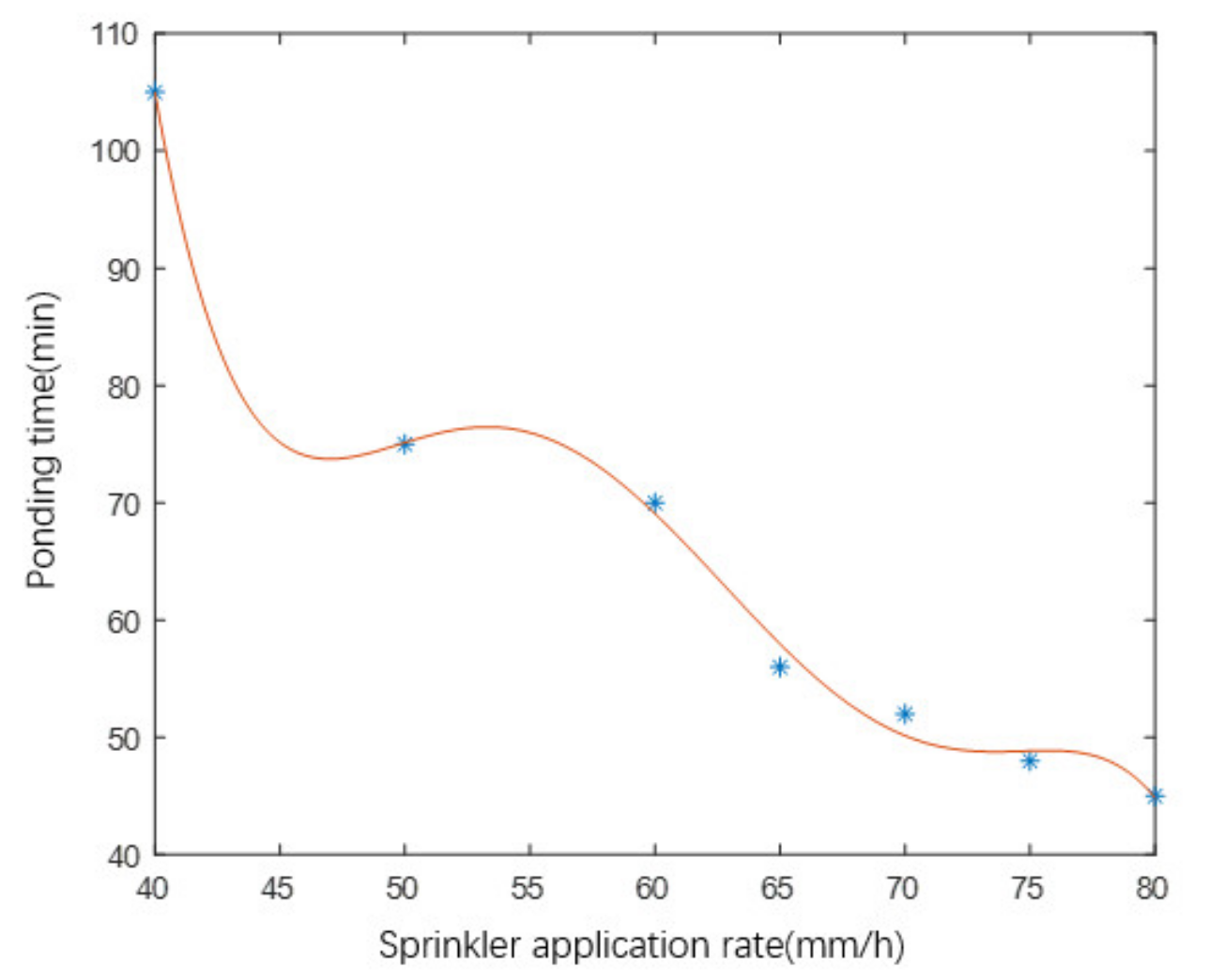
As shown in Figure 6, the water accumulation time of the soil decreases significantly with greater application rate of sprinkler irrigation, and the relationship between the application rate of sprinkler irrigation and the time of soil ponding is the most complex. The greater the application rate of sprinkler irrigation the faster the rate of increase in water content of the soil surface layer, the shorter the time required to increase the soil water content from the initial water content to the saturation water content, and the smaller the corresponding water accumulation time.
3. Determination of Neural Network Input and Output Layers
As shown in Figure 7, Figure 8 and Figure 9, a six-input single output structure is used in this paper. The six inputs include the percentage of sand, silt and clay particles in the soil, the total amount of water irrigated, the bulk density of the soil and the initial water content. The percentages of sand, silt and clay in the soil can be summarized as the texture of the soil. The total amount of irrigation water is the result of multiplying the previously simulated water accumulation time by the application rate of sprinkler irrigation. The output of the neural network is the maximum application rate of sprinkler irrigation that does not produce standing water [23].
4. Training Data Pre-Processing
In practice, the data are multidimensional, so their units are often different. If we do not normalize the data, it will lead to too large or too small data of a certain category in the data set, which will lead to a long training time of the neural network, or even failure to converge. In this paper, we normalize the original data to between −1 and 1 by the following formula [12].
N is the number of samples in the data set, Xmin is the minimum of all training samples, and Xmax is the maximum of all training samples. Partially normalized data for total irrigation water are presented in Table 4.
5. Basic Theory of Neural Networks
5.1. BP Neural Network Basic Theory
The BP neural network is a kind of backward propagation neural network, whose computational process mainly consists of two parts: forward propagation and backward gradient optimization [24]. The reverse gradient optimization is to obtain the best neural network parameters by the gradient descent method to minimize the mean squared error between the actual value of forwarding propagation and the target value. The BP neural network structure has three main components, which are the input layer, hidden layer and output layer. In the neuron is the activation function. Its form is shown below [25].
5.2. Generalized Regression Neural Network Theory
Generalized regression neural networks are very similar to radial basis neural networks, but generalized regression neural networks are based on parameter-free regression theory with an additional summation layer [26]. In parameter-free regression the regression of the input random variable vector x to the output random variable y is considered to be represented by the following conditional probability mean [27].
Here, X is a particular measure of the random variable vector x, y(X) refers to the value of y when the input is X.
The joint probability density, f (X, y), can be estimated by using parzen nonparametric estimates of the sample values , for x and y.
Here, n is the sample size, p is the dimensionality of x, and is the smoothness factor.
Bringing Equation (15) into Equation (16), we get the following equation.
The structure of the generalized regression neural network is mainly to implement the function of Equation (17). The generalized regression neural network consists of four layers: input layer, pattern layer, summation layer and output layer, where the number of neurons in the pattern layer is the same as the number of training samples.
The summation layer has two summation methods: a weighted summation and a simple accumulation of neurons connected as one.
The output layer is equal to the summation layer data division, so that the structure of the generalized neural network can realize the function of parameter-free regression.
6. Evaluation Criteria for Neural Networks
In order to evaluate the prediction effect of RBF neural network and other two neural networks on the maximum application rate of sprinkler irrigation, this paper uses the average relative error to evaluate the advantages and disadvantages of several neural networks [28].
where and are the true and predicted values, respectively, and N is the total test data.
7. Training and Comparison
In this paper, the first 90% of the 1376 data sets obtained from the finite element simulation are used as the training set, and the neural network is trained through the training set. The next 10% of the data are used as the test set to test the accuracy of the neural network.
7.1. Neural Network Parameter Determination
The main parameter of BP neural network is the number of neurons in the hidden layer, and in this paper, that number is determined to be eight by empirical formula 20 [29].
Here, h is the training sample data. This paper uses 90% of the finite element data as the training data, so h equals 1238. M is the number of nodes in the input layer, which for this paper is six, so M equals six. I is the number of neurons in the hidden layer.
The main parameter to be adjusted for generalized regression neural networks and RBF neural networks is the smoothness coefficient σ. In this paper, the dichotomous method is used to perform continuous testing and to determine the value of the smoothness parameter based on the magnitude of the average relative error of the test set.
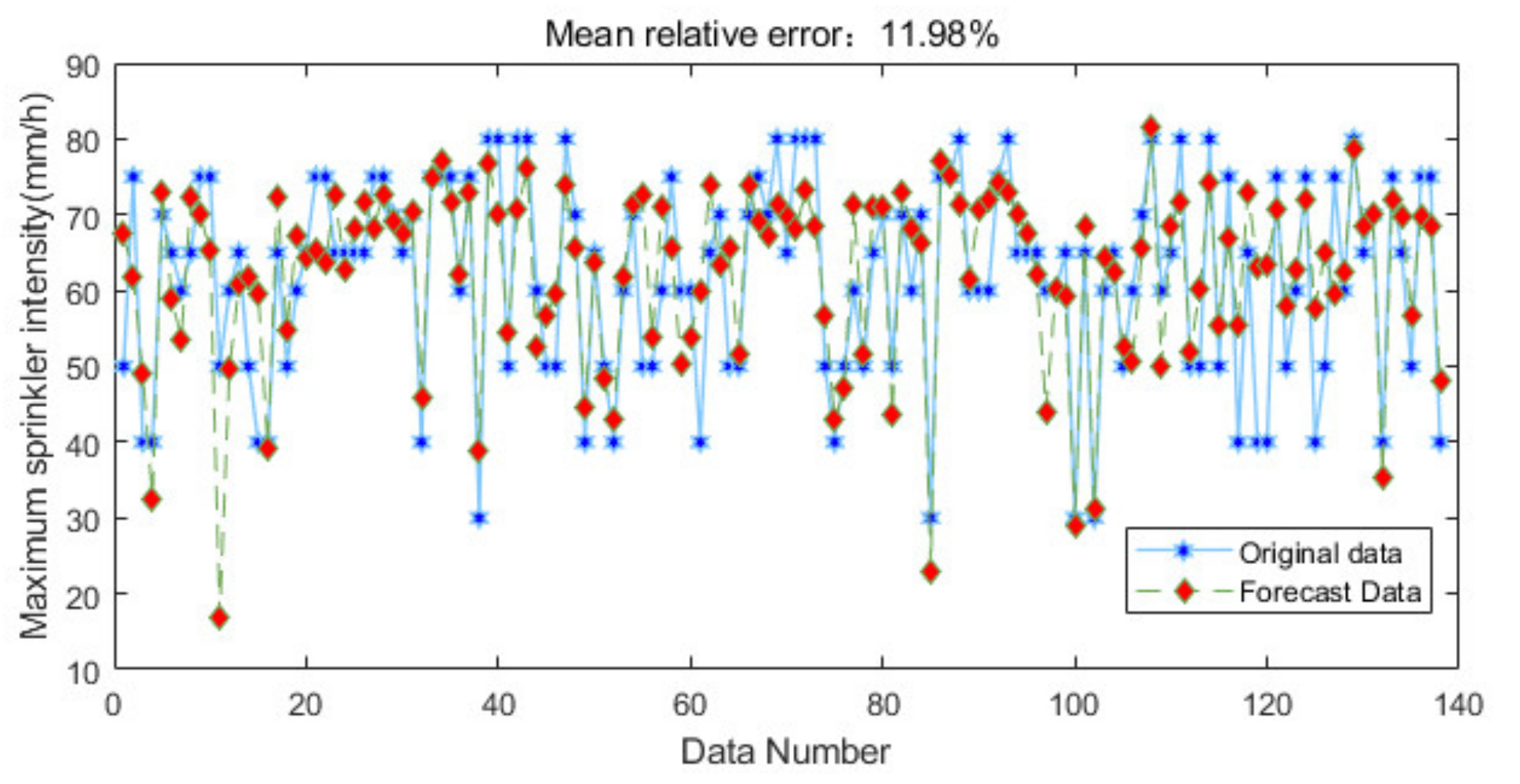
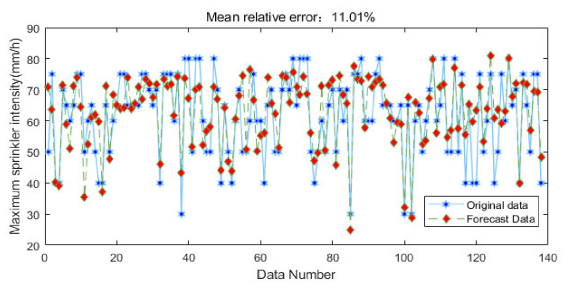
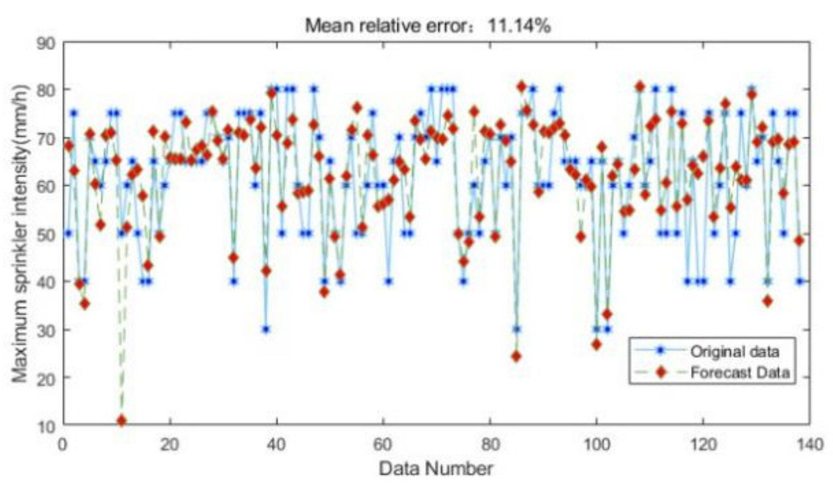
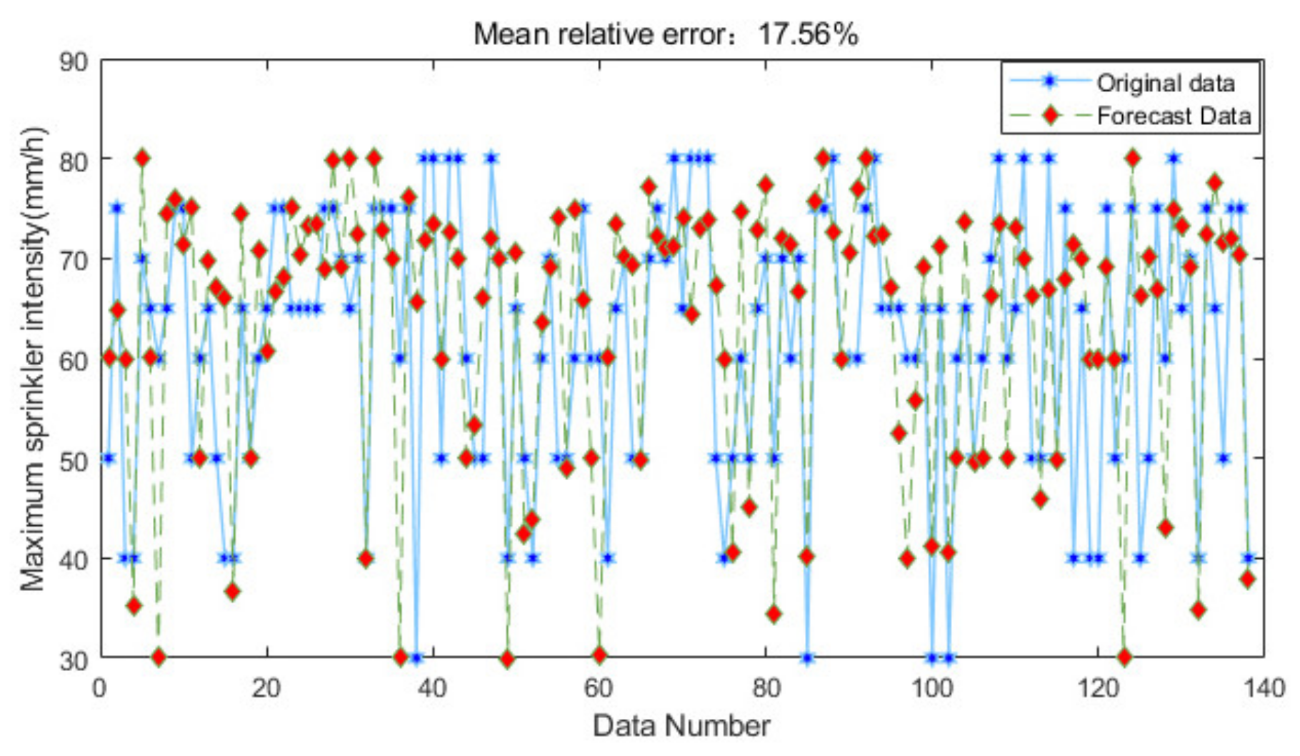
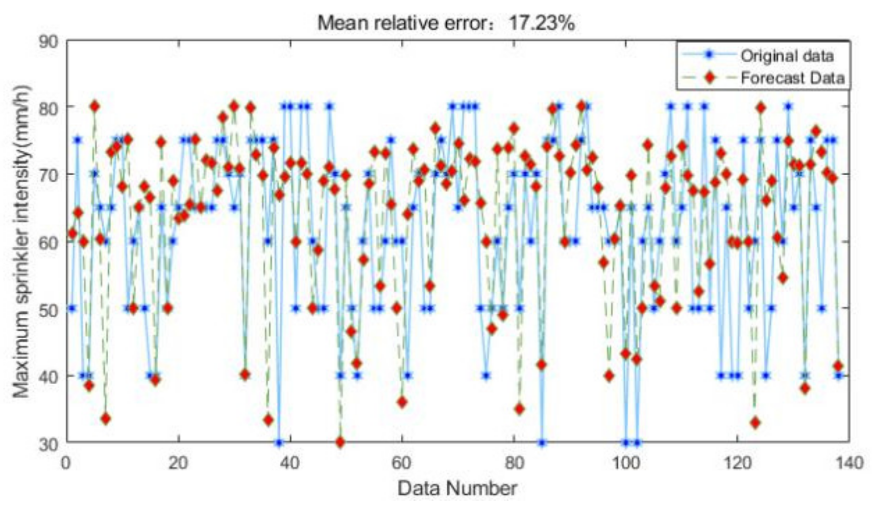
Figure 7, Figure 8 and Figure 9 above show the comparison between the original data of the test set and the predicted data of the RBF neural network when the smoothness parameter of the RBF neural network is 1.15, 1.14 and 1.13, respectively. From the figure, it can be seen that when the smoothness parameter of RBF neural network is 1.14, its average relative error is the smallest, so the smoothness parameter of RBF neural network in this paper is 1.14.
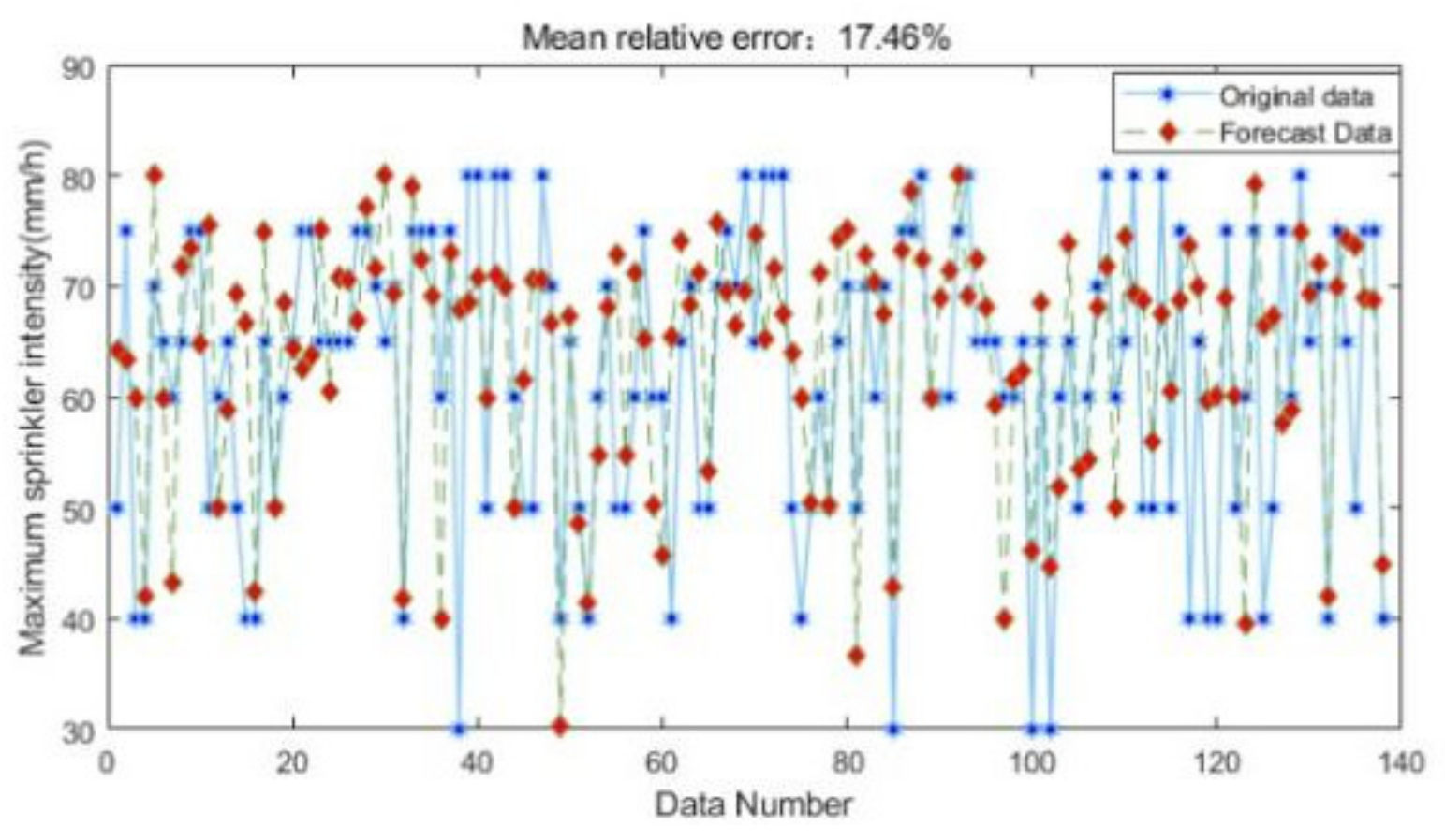
As shown in Figure 10, Figure 11 and Figure 12 above, the original data of the test set is compared with the data predicted by the generalized regression neural network when the smoothness parameters of the generalized regression neural network are 0.02, 0.03 and 0.04, respectively. It can be seen from the figures that when the smoothness parameter of the generalized regression neural network is 0.03, the mean relative error between the original data and the predicted data is the smallest, so the smoothness parameter of the generalized regression neural network in this paper is chosen to be 0.03.
7.2. Comparison of Neural Network Errors
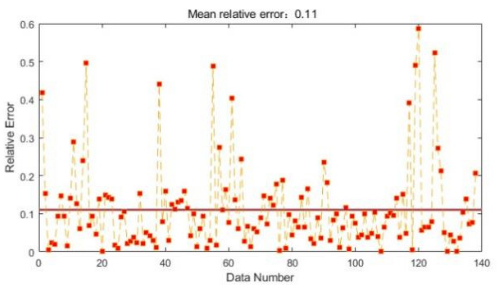
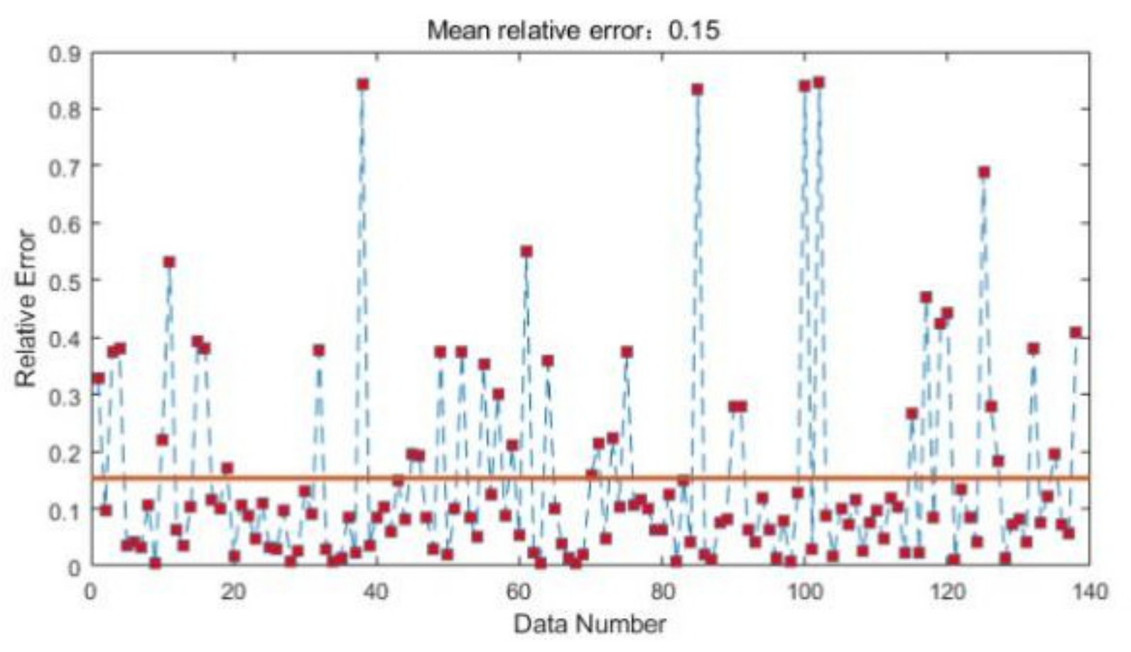
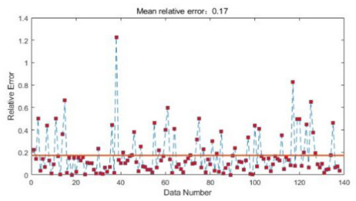
In this chapter, three neural networks are compared and the best one is selected for predicting the maximum application rate of sprinkler irrigation. Figure 13, Figure 14 and Figure 15 show the distribution of the relative errors of the original and predicted data of the test set for the RBF neural network, BP neural network and generalized regression neural network at the optimal parameters, respectively. As shown in the figure, the average relative errors of the three neural networks for the test set of 138 data sets are 0.11, 0.15 and 0.17, respectively. Therefore, the RBF neural network has the lowest average relative error. Meanwhile, the data predicted by the RBF neural network has significantly less error than the BP neural network and the generalized regression neural network. Overall, the relative errors of the BRF neural network prediction data are mostly below 0.1.
In summary, this paper will use RBF neural network to predict the maximum application rate of sprinkler irrigation that does not produce waterlogging in the soil, providing theoretical guidance for the development of the best application rate of sprinkler irrigation for the water and fertilizer integration machine.
8. Empirical Formula for Total Irrigation Water
The total irrigation water requirement m is determined by the depth of irrigation required for different crops and the soil moisture status, and its value can be determined by the empirical Equation (21).
The formula species H is the depth of irrigation determined by the root depth of the crop at different times. is the upper limit of the water content of the soil after irrigation, generally its value is equal to the field water content of the soil. is the lower limit of the water content of the soil before irrigation. is the efficiency of equipment utilization during sprinkler irrigation.
9. Experimental Verification
9.1. Spray Irrigation Soil Infiltration Experiment Site
Soil sprinkler infiltration experiments were conducted from May 2022 to July 2022 at the Engineering Laboratory Building of Guangzhou University (23°030′1.23″ N, 113°240′3.92″ E). The location of the sprinkler infiltration experiment is given in Figure 16. The soil required for the experiments was obtained from the lawn of Guangzhou University with a pH range of 6.62–6.78 [30].
9.2. Experimental Soil Samples
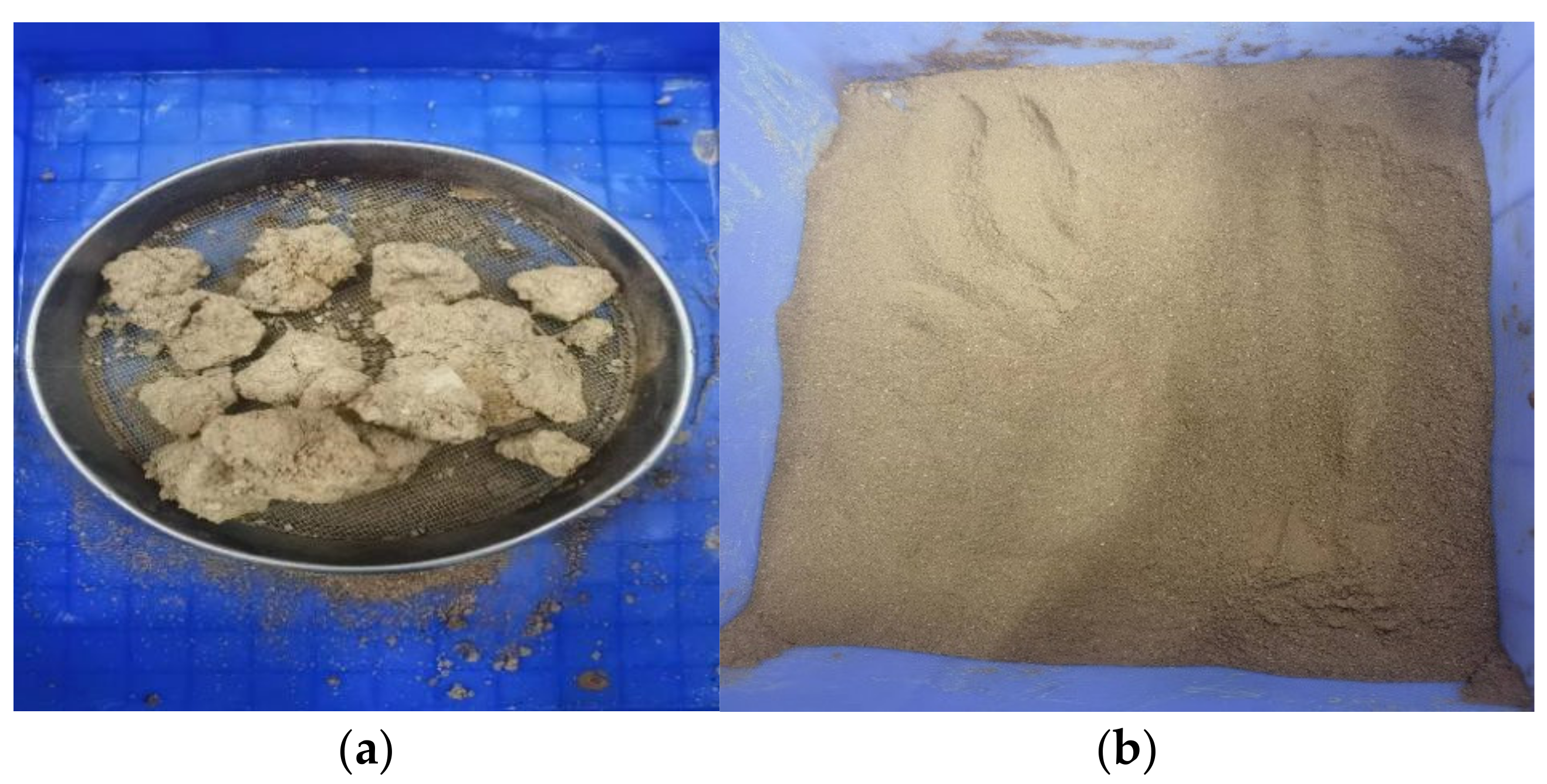
The test soil samples were taken from soils in the 0–20 cm tillage layer in Guangzhou. The soil samples were dried in a dryer and then passed through a fine sieve of 2 mm. Figure 17a,b shows the dried soil block and the soil sample crushed through 2 mm, respectively.
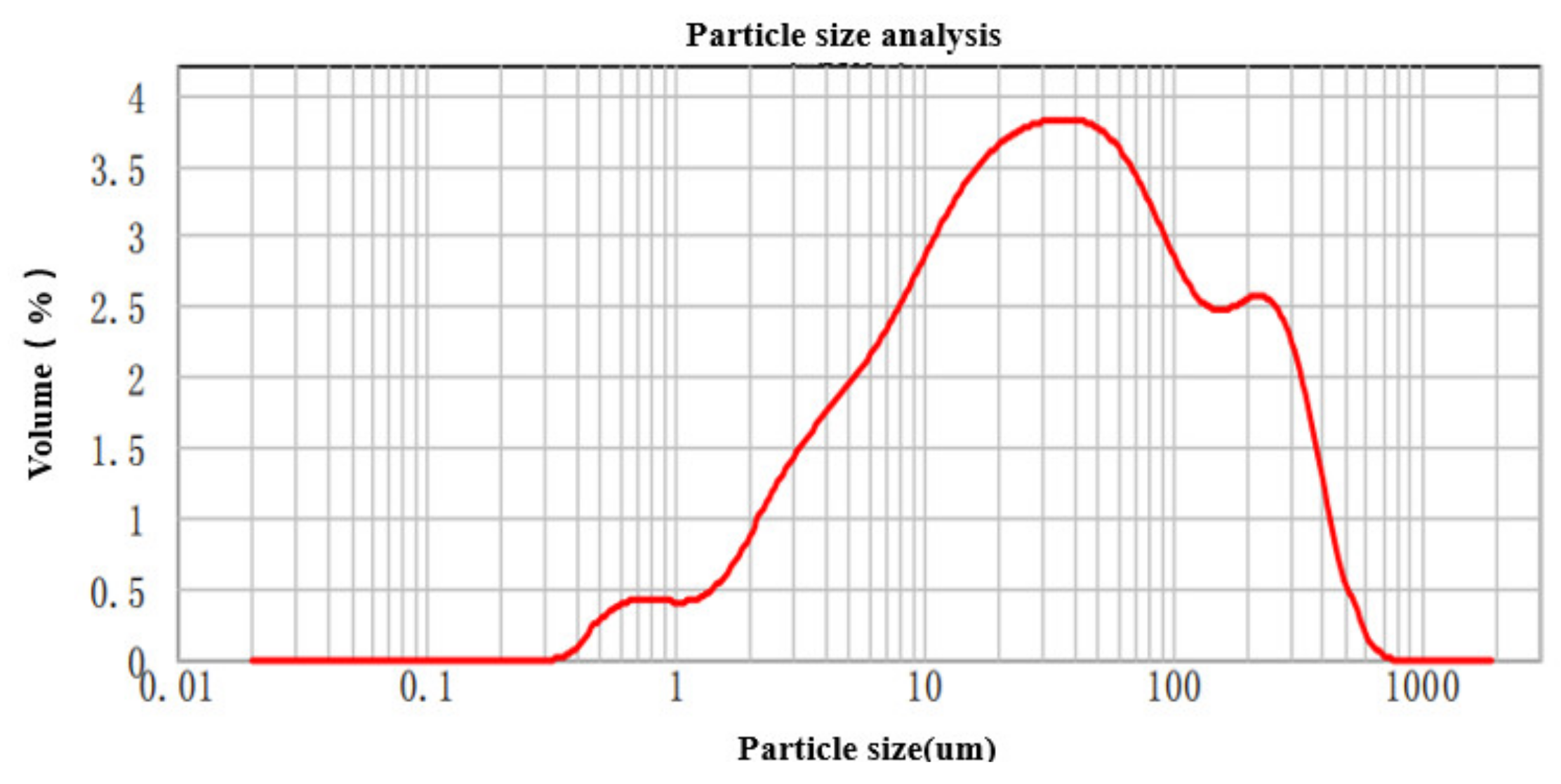
Figure 18 shows the particle size distribution of the sample soil obtained by a laser particle size analyzer. Particles in the soil with diameters between 2 and 0.02 mm are sand particles, between 0.02 and 0.002 mm are silt particles, and less than 0.002 mm are clay particles. Therefore, the percentage of particles in these three intervals was added up, and finally it was determined that the soil sample contains 61.42% sand particles, 34.29% silt particles and 4.29% clay particles, therefore the sample soil was sandy loam [31].
9.3. Construction of Experimental Platform
9.3.1. Soil Infiltration Device
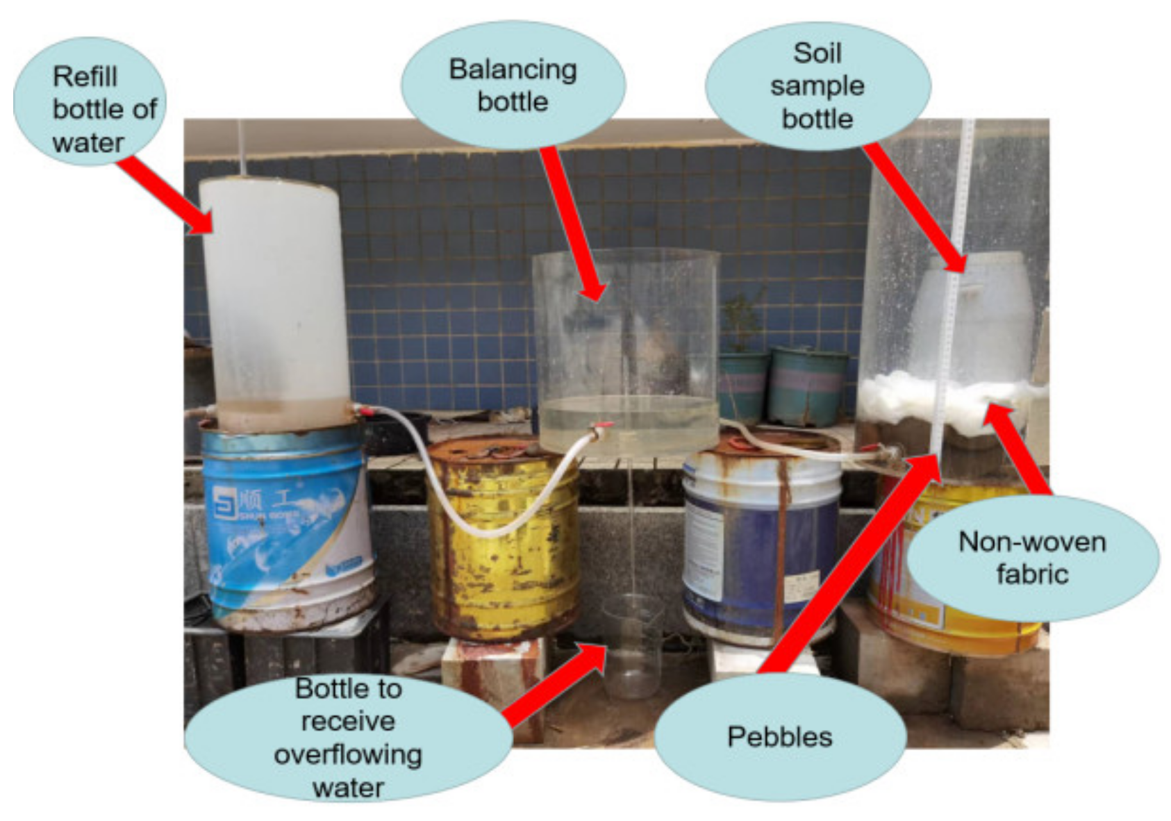
The infiltration device used in this paper is a structured device of a Marriott bottle. As shown in Figure 19, it consists mainly of a soil sample bottle, a balance bottle, a bottle for replenishing water to the balance bottle, and a bottle for receiving water overflow from the balance bottle. The sample bottle is connected to the equilibrium bottle through a hose, the equilibrium bottle is connected to the bottle used for replenishing water through a hose, and the bottle receiving overflow water is connected to the equilibrium bottle through an overflow tube. When the soil is infiltrated, the balance bottle will control the soil water level from changing and the infiltrated water will flow through the overflow tube into the bottle receiving the overflow water. The bottom of the soil sample bottle is a 10 cm thick pebble for filtering groundwater, and a permeable nonwoven fabric is placed on top of the pebble [32].
9.3.2. Sprinkler Irrigation Equipment
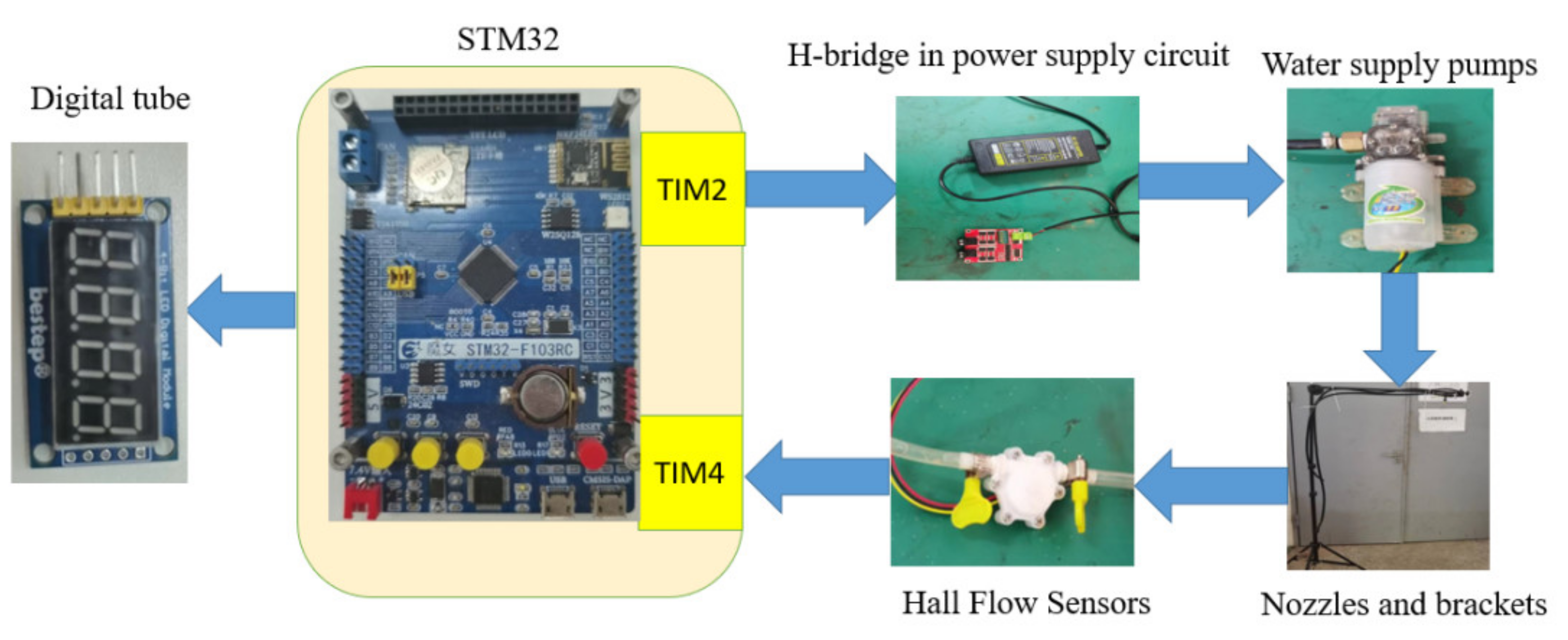
As shown in Figure 20, the system is an application rate of sprinkler irrigation control system with a Hall flow sensor, stm32 controller, H-bridge circuit, pump and nozzle holder as the main components. stm32 is the core controller used to implement the PID control algorithm; the Hall flow sensor transmits the flow data to the microcontroller through the input capture function of stm32’s universal timer TIM4; H-bridge module controls the voltage output through the PWM wave output from the stm32’s general-purpose timer TIM2. This sprinkler application rate control system mainly controls the output flow rate of the pump by controlling the voltage output to the pump from the H-bridge through the microcontroller. The sprinkler application rate is controlled by changing the magnitude of the flow rate. The flow rate of the pump is displayed through a digital tube.
For the Hall flow sensor, when the water flows through it, it drives the rotation of the wheel, which generates pulses. Before using the sensor, the sensor needs to be calibrated. By varying the voltage of the pump, we can measure multiple sets of flow and pulse values of the nozzle in one minute and fit the data to get the relationship between flow and pulse. The relationship between flow and pulse can be expressed by the following equation.
where indicates the number of pulses captured by the microcontroller in one second, and indicates the flow rate in mL/s in one second.
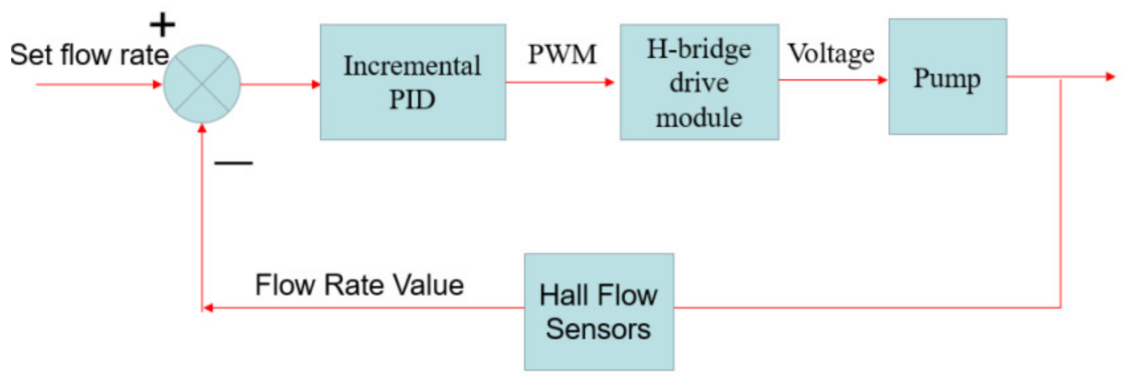
This system uses incremental PID to control the flow rate, and its control block diagram is shown in Figure 21. The duty cycle of the PWM wave output from the timer of the stm32 is adjusted by the difference between the actual flow rate value and the set flow rate value. Then the H-bridge module output voltage value to the pump is adjusted by the different duty cycle to make the pump output the set flow rate. The incremental PID formula is shown below [33].
Bring Equation (25) to (26) to get Equation (27).
where is the output of the system at the nth sampling moment. is the scaling factor, is the differentiation factor, and is the integration factor.
In this system, the trial-and-error method is used to adjust the three parameters of the PID. When is equal to 0.04, is equal to 0.15 and is equal to 0.01, the system works best with a fast response and small overshoot and steady-state error.
9.3.3. Soil Moisture Data Measurement and Transmission System
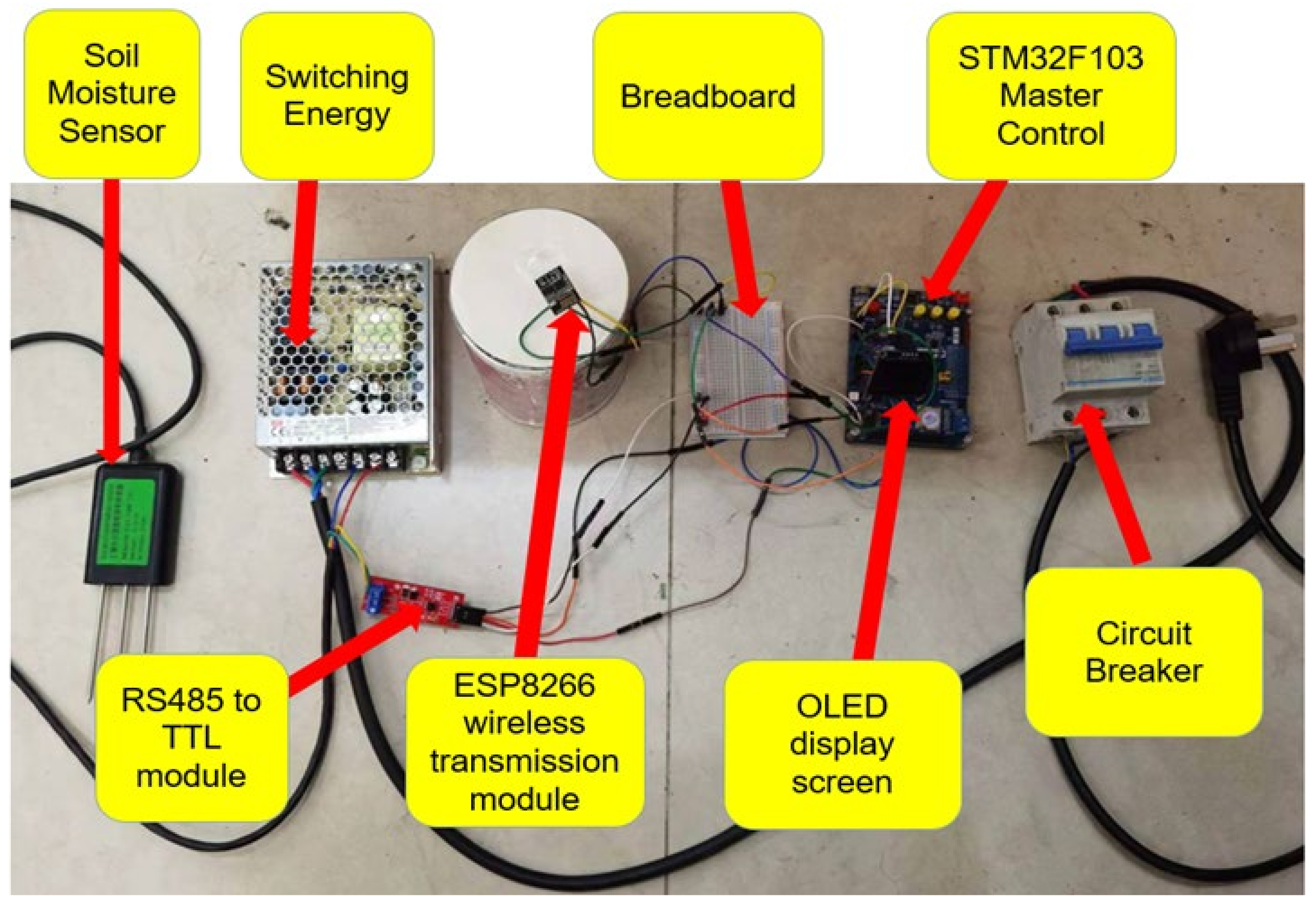
As shown in Figure 22, the system is a soil moisture measurement and transmission module with a moisture sensor, stm32 controller, power switch, RS485 to TTL module, ESP8266 wireless transmission module, breadboard, OLED display and air switch as the main components. The humidity sensor in this paper is from Guangzhou Saiten Technology Company, the data transmission protocol of this sensor is Mod-bus communication protocol, and its interface is a differential structure RS485 structure. In this paper, RS485 to TTL module is used to convert the differential signal of the humidity sensor RS485 to the TTL level signal readable by stm32. The humidity sensor is powered by a switching power supply that can provide 12 V voltage. In order to prevent short circuit or leakage to the equipment and personnel damage, an air switch is added in front of the switching power supply. stm32 microcontroller reads the value of the humidity sensor, then the data is processed and displayed on the OLED display screen and sent to the computer through the ESP8266 wireless module.
9.4. Experimental Steps
The soil for this experiment was obtained from the lawn of Guangzhou University, and its collection process and soil texture analysis have been described in detail in 8.1 above. There, it is known that the soil used for the experiment is a sandy loam. In the experiment, application rate of sprinkler irrigation, soil bulk density and initial water content were selected as independent variables and water accumulation time as dependent variable. The total irrigation volume in the above neural network is obtained by multiplying the water accumulation time by the application rate of sprinkler irrigation. The total irrigation volume, soil bulk density and initial water content are brought into the previously trained neural network to predict an application rate of sprinkler irrigation. The predicted application rate is compared with the set application rate of sprinkler irrigation to verify the effectiveness of the neural network prediction in practice. The parameters of the independent variables are selected as shown in Table 5.
- (1)
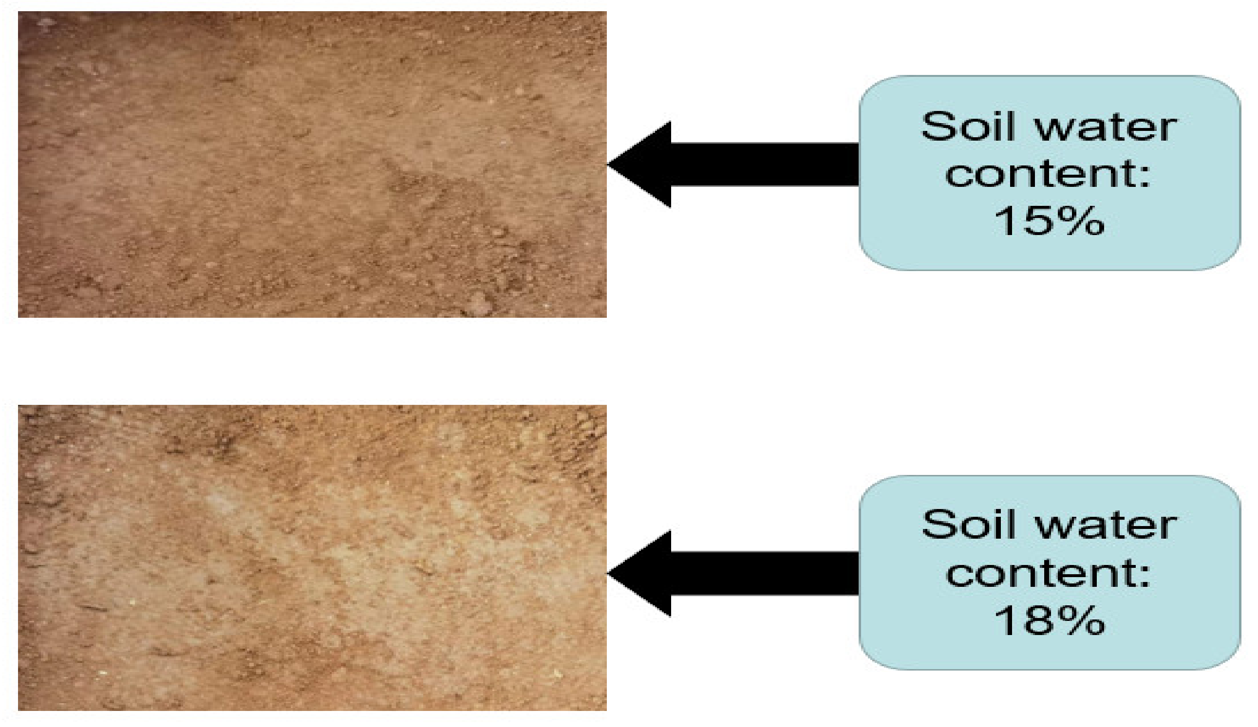
- As shown in Figure 23, the amount of water required to dry the soil to the moisture content in the table was calculated based on the initial soil moisture content listed in Table 5. The soil is then spread out and the water is sprayed evenly on top of the soil to ensure uniformity of soil moisture content.
- (2)
- The soil with the required initial moisture content was left to stand for 24 h and then filled into the soil sample bottles at 2 cm intervals according to the soil bulk density given in Table 5.
- (3)
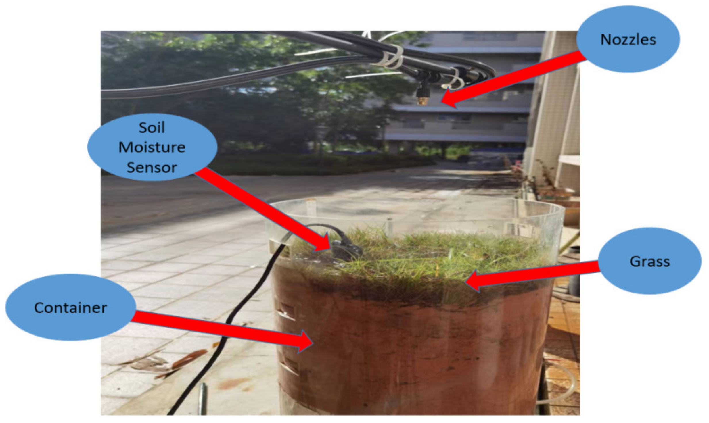
- As shown in Figure 24, at the top end of the soil sample bottle, the soil surface is covered with another layer of grass to simulate crop interception.
- (4)
- (5)
9.5. Comparison of Neural Network Prediction Results with the Actual Situation
RBF neural network predictions were performed for the eight cases in Table 5. Soil quality, total irrigation volume, soil capacity and initial soil moisture content were used as inputs for predicting application rate of sprinkler irrigation, and the predicted application rate of sprinkler irrigation was compared with the application rate of sprinkler irrigation in Table 5 to judge the prediction effectiveness of the RBF neural network. The results of the RBF neural network prediction are shown in Table 7.
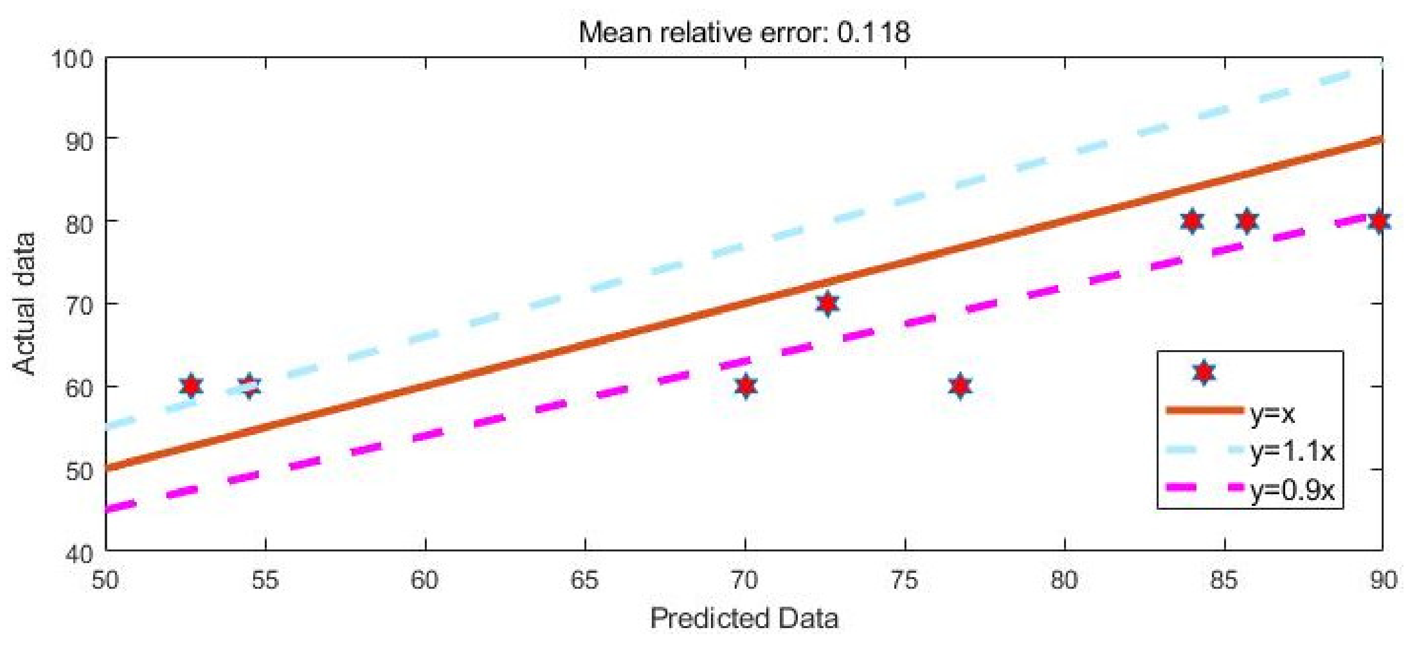
The error analysis of the application rate of sprinkler irrigation predicted by the RBF neural network and the actual application rate of sprinkler irrigation is shown in Figure 25, from which it can be seen that the predicted results of the BF neural network have some deviation from the actual application rate of sprinkler irrigation, but its relative error is about 10% in general, of which the maximum relative error is 27%. Therefore, the RBF neural network has some application value in predicting the maximum application rate of sprinkler irrigation of soil.
10. Value Evaluation Using Optimal Spray Intensity
This paper uses a lawn as an example to verify the advantages of irrigation at optimum application rate of sprinkler irrigation (maximum application rate of sprinkler irrigation without runoff) compared to conventional sprinkler theory. Tall fescue is often used as urban lawn, its soil water absorption condition can be divided into three layers: active layer (0 to 20 cm), sub-active layer (20 to 50 cm), and stable layer (50 to 100 cm). Therefore, the selected wetting depth is 35 cm, and the upper limit of irrigation is assumed to be 30% of the field water holding capacity, and the lower limit of irrigation is 0.5 times of the field water holding capacity. The sprinkler efficiency is 0.9. Bringing the above parameters into the equation mentioned in Section 7, the total irrigation water required is calculated to be 58 mm. From Section 9.2, it is known that the experimental soil is sandy loam, and according to the previous theory of application rate of sprinkler irrigation, it is recommended to use the stable infiltration rate of soil as the application rate of sprinkler irrigation. For sandy loam soil, the recommended application rate is 12 mm/h, while the optimal application rate of sprinkler irrigation predicted by the neural network is 42 mm/h. It takes 4.8 h to irrigate 58 mm using the conventional stable infiltration rate, while it takes only 1.4 h to irrigate 58 mm using the optimal application rate of sprinkler irrigation predicted by the neural network. This shows that the optimal application rate of sprinkler irrigation predicted by the neural network can save 3.4 h, which increases the overall efficiency of the water–fertilizer sprinkler by about 70%. Since irrigation can be completed in a shorter period, it can avoid waste of electricity and unnecessary extension of irrigation time, and reduce evaporation losses while reducing the operation and maintenance costs of the water–fertilizer integrator.
11. Conclusions
A prediction model for the optimal application rate of sprinkler irrigation was developed by establishing a soil infiltration model for sprinkler irrigation using finite elements, neural networks and a total irrigation volume equation. The main conclusions are as follows:
- (1)
- In this paper, the highest accuracy of the optimal sprinkler application rate predicted by RBF neural network is obtained by trial and error method when the smoothing parameter is 1.14. The average relative error of its prediction is 0.11 and the RBF neural network is compared with BP neural network and generalized regression neural network. It can be found that the RBF neural network has the highest prediction accuracy. This indicates that RBF neural network is more suitable for the prediction of sprinkler application rate than other neural networks.
- (2)
- Comparing the experimental data with the prediction results, the relative error of RBF neural network prediction is around 10%. This indicates that the RBF neural network has some practical value in the prediction of sprinkler application rate.
- (3)
- The RBF neural network not only predicts the best sprinkler application rate with high accuracy, but also its fast computing speed makes it ideal for placement into embedded devices.
- (4)
- Among the initial soil water content, bulk density and sprinkler application rate, the most complex effect on soil water accumulation time is the sprinkler application rate.
- (5)
- The finite element values simulated by the soil infiltration model established by the partial differential equation do not differ much from the actual values. Therefore, applying the finite element method to soil infiltration can greatly reduce the complexity of soil infiltration experiments.
- (6)
- The maximum application rate of sprinkler irrigation predicted by combining the RBF neural network with the total irrigation volume formula was compared with the conventional recommended application rate of sprinkler irrigation in actual sprinkler irrigation using the lawn as an example. When the optimal application rate of sprinkler irrigation proposed in this paper was used, the sprinkler time was greatly reduced. For an irrigation volume of 58 mm, for example, the optimal application rate of sprinkler irrigation saves 3.4 h and improves the overall efficiency by about 70%, which greatly reduces irrigation losses due to long sprinkler time and also reduces the operation and maintenance costs of the equipment.
As long as the soil texture, initial moisture content, application rate of sprinkler irrigation, bulk density and total irrigation volume are input into the neural network, the optimal application rate of sprinkler irrigation can be predicted, but its overall accuracy still needs to be improved, the soil studied in this paper is mainly sandy loam in order to improve its application scenario needs to be expanded for other soil textures.
Author Contributions
Conceptualization, T.Z.; methodology, X.Z.; validation, Z.L. and X.L.; resources, Z.L. All authors have read and agreed to the published version of this manuscript.
Funding
The authors acknowledge the funding received from the following science foundations: National Natural Science Foundation of China (51975136, 52075109), National Key Research and Development Program of China (2018YFB2000501), the Science and Technology Innovative Research Team Program in Higher Educational Universities of Guangdong Province (2017KCXTD025), Special Research Projects in the Key Fields of Guangdong Higher Educational Universities (2019KZDZX1009), the Science and Technology Research Project of Guangdong Province (2017A010102014), the Industry-University-Research Cooperation Key Project of Guangzhou Higher Educational Universities (202235139), and Guangzhou University Research Project (YJ2021002).
Data Availability Statement
The data that support the findings of this study are available from the corresponding author upon reasonable request.
Acknowledgments
We thank the referees for their comments and valuable suggestions that helped to improve this paper.
Conflicts of Interest
The authors declare no conflict of interest.
References
- Zhang, K.; Song, B.; Zhu, D.L. The Influence of Sinusoidal Oscillating Water Flow on Sprinkler and Impact Kinetic Energy Intensities of Laterally-Moving Sprinkler Irrigation Systems. Water 2019, 11, 1325. [Google Scholar] [CrossRef]
- Maraseni, T.N.; Mushtaq, S.; Reardon-Smith, K. Re-evaluating the rationale for irrigation technology adoption through an integrated trade-off analysis: Case study of a cotton farming system in Australia. J. Water Clim. Chang. 2014, 5, 328–340. [Google Scholar] [CrossRef]
- Zhang, L.; Fu, B.Y.; Ren, N.W.; Huang, Y. Effect of Pulsating Pressure on Water Distribution and Application Uniformity for Sprinkler Irrigation on Sloping Land. Water 2019, 11, 13. [Google Scholar] [CrossRef]
- Arnold, J.G.; Moriasi, D.N.; Gassman, P.W.; Abbaspour, K.C.; White, M.J.; Srinivasan, R.; Santhi, C.; Harmel, R.D.; Griensven, A.V.; Liew, M.W.V. MT3DMS: Model Use, Calibration, and Validation. Trans. Asabe 2012, 55, 1549–1559. [Google Scholar] [CrossRef]
- Gencoglan, C.; Gencoglan, S.; Merdun, H.; Ucan, K. Determination of ponding time and number of on-off cycles for sprinkler irrigation applications. Agric. Water Manag. 2005, 72, 47–58. [Google Scholar] [CrossRef]
- Espinosa, F.E.C.; Torres, P.; Feyen, J. Experimental assessment of the sprinkler application rate for steep sloping fields. J. Irrig. Drain. Eng. ASCE 2007, 133, 276–278. [Google Scholar] [CrossRef]
- Dadhich, S.M.; Singh, R.P.; Mahar, P.S. Saving time in sprinkler irrigation application through cyclic operation: A theoretical approach. Irrig. Drain. 2012, 61, 631–635. [Google Scholar] [CrossRef]
- DeBoer, D.W.; Chu, S.T. Sprinkler technologies, soil infiltration, and runoff. J. Irrig. Drain. Eng. ASCE 2001, 127, 234–239. [Google Scholar] [CrossRef]
- Trejo-Alonso, J.; Fuentes, C.; Chavez, C.; Quevedo, A.; Gutierrez-Lopez, A.; Gonzalez-Correa, B. Saturated Hydraulic Conductivity Estimation Using Artificial Neural Networks. Water 2021, 13, 705. [Google Scholar] [CrossRef]
- D’Emilio, A.; Aiello, R.; Consoli, S.; Vanella, D.; Iovino, M. Artificial Neural Networks for Predicting the Water Retention Curve of Sicilian Agricultural Soils. Water 2018, 10, 1413. [Google Scholar] [CrossRef] [Green Version]
- Dehghanisanij, H.; Emami, S.; Achite, M.; Linh, N.T.T.; Pham, Q.B. Estimating Yield and Water Productivity of Tomato Using a Novel Hybrid Approach. Water 2021, 13, 3615. [Google Scholar] [CrossRef]
- Gu, J.; Yin, G.H.; Huang, P.F.; Guo, J.L.; Chen, L.J. An improved back propagation neural network prediction model for subsurface drip irrigation system. Comput. Electr. Eng. 2017, 60, 58–65. [Google Scholar] [CrossRef]
- Chen, Z.L.; Zhao, C.J.; Wu, H.R.; Miao, Y.S. A Water-saving Irrigation Decision-making Model for Greenhouse Tomatoes based on Genetic Optimization T-S Fuzzy Neural Network. KSII Trans. Internet Inf. Syst. 2019, 13, 2925–2948. [Google Scholar]
- Al-Naji, A.; Fakhri, A.B.; Gharghan, S.K.; Chahl, J. Soil color analysis based on a RGB camera and an artificial neural network towards smart irrigation: A pilot study. Heliyon 2021, 7, 9. [Google Scholar] [CrossRef]
- Perea, G.; Poyato, C.; Montesinos, P.; Diaz, J.A.R. Prediction of applied irrigation depths at farm level using artificial intelligence techniques. Agric. Water Manag. 2018, 206, 229–240. [Google Scholar] [CrossRef]
- Cao, C.; Song, S.Y.; Chen, J.P.; Zheng, L.J.; Kong, Y.Y. An Approach to Predict Debris Flow Average Velocity. Water 2017, 9, 205. [Google Scholar] [CrossRef]
- Wei, D.F. Network traffic prediction based on RBF neural network optimized by improved gravitation search algorithm. Neural Comput. Appl. 2017, 28, 2303–2312. [Google Scholar] [CrossRef]
- Arbat, G.; Puig-Bargues, J.; Barragan, J.; Bonany, J.; de Cartagena, F.R. Monitoring soil water status for micro-irrigation management versus modelling approach. Biosyst. Eng. 2008, 100, 286–296. [Google Scholar] [CrossRef]
- Aster, R.C.; Thurber, C.H.; Borchers, B. Parameter Estimation and Inverse Problems; Elsevier: Amsterdam, The Netherlands, 2011. [Google Scholar]
- Mi, L.; Luo, W. An Approximate Analytical Solution of Van Genuchten Model. In Proceedings of the 2017 2nd International Symposium on Advances in Electrical, Electronics and Computer Engineering (ISAEECE 2017), Guangzhou, China, 25–26 March 2017. [Google Scholar]
- Mao, Y.W.; Liu, S.; Nahar, J.; Liu, J.F.; Ding, F. Soil moisture regulation of agro-hydrological systems using zone model predictive control. Comput. Electron. Agric. 2018, 154, 239–247. [Google Scholar] [CrossRef]
- Lei, W.K.; Dong, H.Y.; Chen, P.; Lv, H.B.; Fan, L.Y.; Mei, G.X. Study on Runoff and Infiltration for Expansive Soil Slopes in Simulated Rainfall. Water 2020, 12, 19. [Google Scholar]
- Yang, G.; Wu, X.P.; Song, Y.X.; Chen, Y.C. Fault diagnosis of complicated machinery system based on genetic algorithm and fuzzy RBF neural network. In Advances in Natural Computation; Jiao, L., Wang, L., Gao, X., Liu, J., Wu, F., Eds.; Lecture Notes in Computer Science; Springer-Verlag: Berlin, Germany, 2006; Volume 4222, Pt 2, pp. 908–917. [Google Scholar]
- Chen, S.Y.; Fang, G.H.; Huang, X.F.; Zhang, Y.H. Water Quality Prediction Model of a Water Diversion Project Based on the Improved Artificial Bee Colony-Backpropagation Neural Network. Water 2018, 10, 806. [Google Scholar] [CrossRef]
- Wang, Z.; Jia, L.M.; Qin, Y.; Wang, Y. Railway passenger traffic volume prediction based on neural network. Appl. Artif. Intell. 2007, 21, 1–10. [Google Scholar]
- Cai, H.H.; Wu, Z.H.; Huang, C.; Huang, D.Z. Wind Power Forecasting Based on Ensemble Empirical Mode Decomposition with Generalized Regression Neural Network Based on Cross-Validated Method. J. Electr. Eng. Technol. 2019, 14, 1823–1829. [Google Scholar] [CrossRef]
- Firat, M.; Gungor, M. Generalized Regression Neural Networks and Feed Forward Neural Networks for prediction of scour depth around bridge piers. Adv. Eng. Softw. 2009, 40, 731–737. [Google Scholar] [CrossRef]
- Zhang, F.Q.; Wu, S.Y.; Wang, Y.O.; Xiong, R.; Ding, G.Y.; Mei, P.; Liu, L.Y. Application of Quantum Genetic Optimization of LVQ Neural Network in Smart City Traffic Network Prediction. IEEE Access 2020, 8, 104555–104564. [Google Scholar] [CrossRef]
- Deng, D.; Zhao, W.W.; Wan, D.C. Vortex-induced vibration prediction of a flexible cylinder by three-dimensional strip model. Ocean Eng. 2020, 205, 17. [Google Scholar] [CrossRef]
- Liang, Z.W.; Liu, X.C.; Zou, T.; Xiao, J.R. Adaptive Prediction of Water Droplet Infiltration Effectiveness of Sprinkler Irrigation Using Regularized Sparse Autoencoder-Adaptive Network-Based Fuzzy Inference System (RSAE-ANFIS). Water 2021, 13, 791. [Google Scholar] [CrossRef]
- Zobeck, T.M. Rapid soil particle size analyses using laser diffraction. Appl. Eng. Agric. 2004, 20, 633–639. [Google Scholar] [CrossRef]
- Li, J.T.; Wa, S.; Song, G.J.; Qiao, X.Y.; Wang, J.H. Modification of Zhengzhou Groundwater Balance Test Site-General Idea and Application Outlook. Hydrogeol. Eng. Geol. 2019, 7. [Google Scholar]
- Chu, C.W.; Zhu, Z.C.; Bian, H.T.; Jiang, J.C. Design of self-heating test platform for sulfide corrosion and oxidation based on Fuzzy PID temperature control system. Meas. Control 2021, 54, 1082–1096. [Google Scholar] [CrossRef]
Figure 1.
RBF neural network structure.

Figure 2.
Spray irrigation soil hydrology system.

Figure 3.
Soil finite element classification.

Figure 4.
Initial moisture content versus time of water accumulation. * is the data points of the finite element simulation, the red line is fitted through the data points.
Figure 4.
Initial moisture content versus time of water accumulation. * is the data points of the finite element simulation, the red line is fitted through the data points.

Figure 5.
Relationship between bulk density and time of soil water accumulation. * is the data points of the finite element simulation, the red line is fitted through the data points.
Figure 5.
Relationship between bulk density and time of soil water accumulation. * is the data points of the finite element simulation, the red line is fitted through the data points.

Figure 6.
The relationship between application rate of sprinkler irrigation and the duration of water accumulation. * is the data points of the finite element simulation, the red line is fitted through the data points.
Figure 6.
The relationship between application rate of sprinkler irrigation and the duration of water accumulation. * is the data points of the finite element simulation, the red line is fitted through the data points.

Figure 7.
The smoothness parameter of the RBF neural network is 1.15.

Figure 8.
The smoothness parameter of the RBF neural network is 1.14.

Figure 9.
The smoothness parameter of the RBF neural network is 1.13.

Figure 10.
The smoothness parameter of the GRNN is 0.02.

Figure 11.
The smoothness parameter of the GRNN is 0.03.

Figure 12.
The smoothness parameter of the GRNN is 0.04.

Figure 13.
Relative error of RBF neural networks. The red line represents the mean relative error.

Figure 14.
Relative error of BP neural networks. The red line represents the mean relative error.

Figure 15.
Relative error of generalized regression neural networks. The red line represents the mean relative error.
Figure 15.
Relative error of generalized regression neural networks. The red line represents the mean relative error.

Figure 16.
Location of sprinkler irrigation experiments at Guangzhou University.

Figure 17.
(a) Drying clay; (b) Fine soil through 2 mm sieve.

Figure 18.
Soil particle size analysis.

Figure 19.
Soil infiltration device.

Figure 20.
System Block Diagram.

Figure 21.
System Block Diagram (incremental PID to control the flow rate).

Figure 22.
Humidity measurement and transmission system.

Figure 23.
Soil moisture.

Figure 24.
Experimental status.

Figure 25.
Error analysis of RBF neural network prediction.


Table 1.
Soil parameters requiring finite element analysis.
| Condition | Sand (%) | Silt (%) | Clay (%) | Soil Texture |
|---|---|---|---|---|
| 1 | 55 | 45 | 0 | Sandy loamy soil |
| 2 | 60 | 30 | 10 | Sandy loamy soil |
| 3 | 64 | 30 | 6 | Sandy loamy soil |
| 4 | 68 | 27 | 5 | Sandy loamy soil |
| 5 | 70 | 15 | 15 | Sandy loamy soil |
| 6 | 75 | 13 | 12 | Sandy loamy soil |
| 7 | 80 | 11 | 9 | Sandy loamy soil |
Table 2.
Initial water content and application rate of sprinkler irrigation.
| Initial Moisture Content (%) | 6 | 9 | 11 | 12 | 14 | 15 | 17 | 18 |
| Application rate of sprinkler irrigation(mm/h) | 30 | 40 | 50 | 60 | 65 | 70 | 75 | 80 |
Table 3.
Partial simulation data.
| Soil Texture | Initial Moisture Content (%) | Bulk Density (g/cm3) | Application Rate of Sprinkler Irrigation (mm/h) | Time of Ponding (min) |
|---|---|---|---|---|
| Condition1 | 6 | 1.5 | 30 | 84 |
| Condition1 | 9 | 1.5 | 30 | 75 |
| Condition1 | 11 | 1.5 | 30 | 69 |
| Condition1 | 12 | 1.5 | 30 | 66 |
| Condition1 | 14 | 1.5 | 30 | 60 |
| Condition2 | 6 | 1.3 | 30 | 169 |
| Condition2 | 6 | 1.4 | 30 | 134 |
| Condition2 | 6 | 1.5 | 30 | 113 |
| Condition2 | 9 | 1.3 | 30 | 156 |
| Condition2 | 9 | 1.4 | 30 | 122 |
| Condition3 | 6 | 1.3 | 40 | 93 |
| Condition3 | 6 | 1.4 | 40 | 83 |
| Condition3 | 6 | 1.5 | 40 | 74 |
| Condition3 | 9 | 1.3 | 40 | 87 |
| Condition3 | 9 | 1.4 | 40 | 76 |
| Condition3 | 9 | 1.5 | 40 | 67 |
| Condition3 | 11 | 1.3 | 40 | 90 |
| Condition4 | 11 | 1.3 | 50 | 62 |
| Condition4 | 11 | 1.4 | 50 | 55 |
| Condition4 | 11 | 1.5 | 50 | 51 |
| Condition4 | 12 | 1.3 | 50 | 69 |
| Condition4 | 12 | 1.4 | 50 | 53 |
| Condition4 | 12 | 1.5 | 50 | 49 |
| Condition4 | 14 | 1.3 | 50 | 62 |
| Condition4 | 14 | 1.4 | 50 | 49 |
Table 4.
Normalized Data Comparison.
| Original data (mm) | 85 | 35 | 76.5 | 24 | 53 | 42 | 60 | 62 | 34.67 |
| Post-processing data (mm) | 1 | −0.64 | 0.72 | −1 | −0.05 | −0.41 | 0.18 | 0.25 | −0.65 |
Table 5.
Experimental variable selection.
| Initial Moisture Content (%) | Bulk Density (g/cm3) | Application Rate of Sprinkler Irrigation (mm/h) |
|---|---|---|
| 15 | 1.3 | 60 |
| 15 | 1.4 | 60 |
| 16 | 1.3 | 60 |
| 18 | 1.3 | 70 |
| 18 | 1.4 | 60 |
| 18 | 1.5 | 80 |
| 18 | 1.4 | 80 |
| 16 | 1.5 | 80 |
Table 6.
Experimental results of water accumulation time.
| Condition | Time of Ponding (min) | Total Irrigation Volume (mm) |
|---|---|---|
| 1 | 56 | 56 |
| 2 | 50 | 50 |
| 3 | 55 | 55 |
| 4 | 40 | 47 |
| 5 | 44 | 44 |
| 6 | 30 | 40 |
| 7 | 32 | 43 |
| 8 | 31 | 41 |
Table 7.
Application rate of sprinkler irrigation predicted by RBF neural network.
| Condition | Predicted Application Rate of Sprinkler Irrigation (mm/h) |
|---|---|
| 1 | 55 |
| 2 | 77 |
| 3 | 53 |
| 4 | 73 |
| 5 | 70 |
| 6 | 84 |
| 7 | 90 |
| 8 | 86 |
Publisher’s Note: MDPI stays neutral with regard to jurisdictional claims in published maps and institutional affiliations. |
© 2022 by the authors. Licensee MDPI, Basel, Switzerland. This article is an open access article distributed under the terms and conditions of the Creative Commons Attribution (CC BY) license (https://creativecommons.org/licenses/by/4.0/).
Share and Cite
MDPI and ACS Style
Liu, X.; Zhu, X.; Liang, Z.; Zou, T. Optimal Sprinkler Application Rate of Water–Fertilizer Integration Machines Based on Radial Basis Function Neural Network. Water 2022, 14, 2838. https://doi.org/10.3390/w14182838
AMA Style
Liu X, Zhu X, Liang Z, Zou T. Optimal Sprinkler Application Rate of Water–Fertilizer Integration Machines Based on Radial Basis Function Neural Network. Water. 2022; 14(18):2838. https://doi.org/10.3390/w14182838
Chicago/Turabian StyleLiu, Xiaochu, Xiangjin Zhu, Zhongwei Liang, and Tao Zou. 2022. "Optimal Sprinkler Application Rate of Water–Fertilizer Integration Machines Based on Radial Basis Function Neural Network" Water 14, no. 18: 2838. https://doi.org/10.3390/w14182838
Note that from the first issue of 2016, this journal uses article numbers instead of page numbers. See further details here.