
Predicting Aquaculture Water Quality Using Machine Learning Approaches
1
School of Resources and Environmental Engineering, Ludong University, Yantai 264025, China
2
CAS Key Laboratory of Coastal Environmental Processes and Ecological Remediation, Yantai Institute of Coastal Zone Research, Chinese Academy of Sciences, Yantai 264003, China
3
Shandong Key Laboratory of Coastal Environmental Processes, Yantai 264003, China
*
Author to whom correspondence should be addressed.
Water 2022, 14(18), 2836; https://doi.org/10.3390/w14182836
Submission received: 27 July 2022
/
Revised: 5 September 2022
/
Accepted: 8 September 2022
/
Published: 12 September 2022
(This article belongs to the Special Issue Advances in Hydrogeology and Groundwater Management Research)
Abstract
:Good water quality is important for normal production processes in industrial aquaculture. However, in situ or real-time monitoring is generally not available for many aquacultural systems due to relatively high monitoring costs. Therefore, it is necessary to predict water quality parameters in industrial aquaculture systems to obtain useful information for managing production activities. This study used back propagation neural network (BPNN), radial basis function neural network (RBFNN), support vector machine (SVM), and least squares support vector machine (LSSVM) to simulate and predict water quality parameters including dissolved oxygen (DO), pH, ammonium-nitrogen (NH3-N), nitrate nitrogen (NO3-N), and nitrite-nitrogen (NO2-N). Published data were used to compare the prediction accuracy of different methods. The correlation coefficients of BPNN, RBFNN, SVM, and LSSVM for predicting DO were 0.60, 0.99, 0.99, and 0.99, respectively. The correlation coefficients of BPNN, RBFNN, SVM, and LSSVM for predicting pH were 0.56, 0.84, 0.99, and 0.57. The correlation coefficients of BPNN, RBFNN, SVM, and LSSVM for predicting NH3-N were 0.28, 0.88, 0.99, and 0.25, respectively. The correlation coefficients of BPNN, RBFNN, SVM, and LSSVM for predicting NO3-N were 0.96, 0.87, 0.99, and 0.87, respectively. The correlation coefficients of BPNN, RBFNN, SVM, and LSSVM predicted NO2-N with correlation coefficients of 0.87, 0.08, 0.99, and 0.75, respectively. SVM obtained the most accurate and stable prediction results, and SVM was used for predicting the water quality parameters of industrial aquaculture systems with groundwater as the source water. The results showed that the SVM achieved the best prediction effect with accuracy of 99% for both published data and measured data from a typical industrial aquaculture system. The SVM model is recommended for simulating and predicting the water quality in industrial aquaculture systems.
1. Introduction
Aquaculture has played an important role in solving the food crisis, ensuring food safety, improving people’s livelihood, and expanding exports. China contributes to major global aquaculture productivity. However, the development of fisheries in China is constrained by both resources and the environment. The resources are increasingly depleted, and the aquatic environment has been affected by multiple pollutants [1,2,3]. Industrial aquaculture is a currently advanced mode with higher breeding density and more yields, but industrial farming is prone to the problems of unscientific feeding and the deterioration of water quality. A temperature of 25–32 degrees Celsius and a pH of 6.5–8.5 are the most suitable for the growth of aquatic animals. The dissolved oxygen (DO) concentration in an aquaculture system should be higher than 5 mg/L. The concentration of NH3-N should be lower than 0.2 mg/L, while that of NO2-N should be generally lower than 0.1 mg/L. In industrial aquaculture systems, especially recirculating systems, the aquatic animals can sustain relatively high concentrations of NH3-N, NO2-N, and NO3-N to some extent. The long-term breeding results have showed that the cultured animals grew well when the ammonia-nitrogen in the recirculating water was lower than 0.4 mg/L. The maintenance of good water quality in aquaculture systems is closely affected by real-time water quality monitoring and accurate water quality prediction. Real-time water quality monitoring or measurement of water quality parameters such as nitrate, nitrite, and ammonia are generally expensive for aquaculture farms. Thus, accurate water quality simulation and prediction are good choices for most industrial aquaculture farms. It is of great economic value to discuss the feasibility of mathematical methods of water quality prediction [4,5]. Good water quality prediction will well maintain the stability of aquaculture systems and reduce the occurrence of fish diseases caused by water quality deterioration.
Water quality prediction methods can be classified under two main categories including traditional prediction methods and machine-learning (ML) models. Traditional water quality prediction methods have the advantage of being easy to implement [6]. However, traditional methods cannot capture nonlinear [7] and nonstationary [8] data on water quality. ML, which is an advanced method of prediction, has globally become a popular research topic and been successfully developed for water quality prediction. ML methods include artificial neural network (ANN) models, support vector machine (SVM), decision tree (DT), random forest (RF), extreme gradient boosting (XGBoost), and other novel models. ANN models are developed on the basis of neural networks in organisms. ANN learning algorithms include back propagation (BP), perceptron algorithm, extreme learning machine (ELM), and radial basis function network (RBF). ANNs have been widely used in the field of water quality prediction. Marcus et al. predicted the weekly nitrate-nitrogen concentration in the Sangamon River near Decatur, Illinois, USA, using an ANN model and compared it with a linear regression model [9]. Suen and Eheart compared two different ANN models (BPNN and RBFNN) for the prediction of nitrate concentrations in the Upper Sangamon River Basin in Illinois, USA [10]. R2 of BPNN ranged from 78% to 83% with RMSE of 2.05–2.317, while that of RBFNN ranged from 75% to 83% with RMSE of 2.567–2.946 [10]. Xu et al. compared three prediction models including time series, multiple linear regression, and BPNN to find that BPNN obtained the best prediction result [11]. SVM, which is a representative statistical-learning algorithm, can establish a linearly separated hyperplane for data classification. SVM is very robust for overfitting. SVM algorithms include support vector regression (SVR) and least square support vector machine (LSSVM). The SVR model can fit the input–output relationship of a simulation model to a high degree with less computation with MAE in the range of 0.57–3.3 [12]. LSSVM using RBF as a kernel function was found to be the best model with the highest R2 of 77% [13]. A LSSVM model was utilized for modeling the discharge-suspended sediment relationship to achieve good performance with R2 in the range of 90.9–96% [14]. ANN and SVM were previously used for predictions of algal growth [15]. The results revealed that ANN achieved satisfactory results with quick response, while the SVM was suitable for accurately identifying the optimal model but taking longer training time [15]. Mirarabi et al. reported that the SVR model performed better than the ANN model for 1-, 2-, and 3-month ahead groundwater-level forecasting, while the SVR model could be successfully used in predicting monthly groundwater in confined and unconfined systems [16]. SVR and ANN were also used to predict flood, and the results showed that the predictions of the SVR model for different magnitudes of floods were similar and relatively constant, whereas the ANN model tended to overpredict the smaller floods and underpredicted the extreme floods [17]. RF usually uses a bootstrap with a random subset to be suitable for more variables, while XGBoost is a boosting algorithm. Both RF and XGBoost belong to decision-tree-based machine learning methods with big datasets and high efficiency [18]. In general, the predictions of these methods achieved different accuracies, with R2 ranging from 40 to 96% [10,11,12,13,14,15]. Good prediction performance is related to multiple factors and requires careful method screening.
Although scientists have conducted a great deal of research on water quality prediction, predicting the water quality in factory farming using small amounts of data is not enough. The amount of water quality data in industrial farming systems is generally small due to the relatively high monitoring cost. Real-time monitoring on industrial farms is also often missing. Therefore, it is important to predict water quality for small-scale industrial farms using small sample data. Artificial neural network was first selected by considering the general applicability of the model. Four representative models were selected to simulate and predict water quality, and the prediction accuracy of each method was compared. Finally, the model with the best prediction accuracy was selected to predict the water quality of a real aquaculture system with groundwater as the source water. The goal of this study was to select the machine learning model with the best performance for water quality prediction in industrial aquaculture systems.
2. Material and Methods
2.1. Selection of Water Quality Prediction Model
ANN is a well-developed machine learning model with high nonlinear fitting ability and self-learning ability. BPNN is one of the most commonly used models in machine learning with unique characteristics. BPNN does not have local minimum problems. SVM can overcome the shortcomings of BPNN, such as poor repeatability and overfitting. SVR has strong generalization ability for small datasets, and it does not require a priori definitions of architecture. The structural risk minimization principle gives SVR the unique advantage of not reducing the prediction accuracy and operating efficiency in dealing with the data of unknown changes so that it is more suitable for the prediction of water quality parameters. LSSVM is an improved method based on SVR. This study also used XGBoost and RF for method prescreening. The pretest results showed that the accuracy of XGBoost/RF was below 40% and much lower than that of ANN and SVM. Therefore, XGBoost and RF were not used for further investigation. This study finally selected BPNN, RBFNN, SVM, and LSSVM models as water quality prediction models.
2.1.1. Back Propagation Neuron Network (BPNN)
BPNN is a widely used neural network method that is an intelligent information processing system [19]. BPNN input data are trained according to the error back-propagation algorithm. BPNN belongs to a multilayer feed-forward network that uses gradient descent to achieve the best value for prediction. The BPNN generally has a structure of three layers including the input layer, the hidden layer, and the output layer. BPNN uses a sigmoid nonlinear function as the transfer function [20] with the following equation:
BPNN can implement predictions directly through the MATLAB toolbox. The BP neural network predicts through the Fitting app in MATLAB, in which the Levenberg–Marguardt algorithm is used [21].
2.1.2. Radial Basis Function Neuron Network (RBFNN)
RBFNN, with neural network structures that mimic human brain sensations, is a three-layer feed-forward network with a single hidden layer. It has a simple network structure, simple training, and fast learning convergence. RBFNN is a local approximation network that uses RBFNN to speed up learning and avoid local mini-problems so that it is suitable for real-time control needs [22,23].
An RBFNN consists of three parts including an input layer consisting of a set of perception units, an implicit layer of compute nodes, and an output layer of a compute node. The hidden layer of the RBF network adopts the radial basis function as the nonlinear transformation function, namely:
where xp is the p-th input sample, ci is the i-th center point, and h is the number of nodes in the hidden layer. For the radial basis function, its main parameters are the function center ci, width σi, and hidden layer weights ωi. At the output layer, the RBF network obtains the output through a linear transformation:
where n is the number of samples to output and ω is hidden layer weights.
First, the center of the radial basis function needs to be determined. The self-organized center selection method is a common algorithm for determining the center, which belongs to unsupervised learning and is also known as tutorless learning. This study determined the center ci of each implied node by k-means clustering:
where ni is the total number of samples participating in the training or test and Xm represents the k-th cluster center. Clustering stops when the change in the center of the class is less than the preset constant.
The basic function selects the Gaussian function, and the width σi can be solved by the following equation:
where cmax is the maximum distance between the selected center.
After the center and width of the hidden layer nodes are determined, the output weight vector can be calculated using pseudo-inverse, least squares, and gradient descent.
2.1.3. Support Vector Regression Machine (SVM)
Vapnik et al. [24] introduced ε insensitive loss function on the basis of SVM classification to obtain a support vector regression machine (SVR) and achieved good performance. The basic idea of SVR is to find an optimal classification surface so that all training samples have the least error from the optimal classification surface [25].
Let the sample set be (xi,yi), i = 1, 2, …, n, where xi (xi∈Rn) is the input value of the i sample, and yi∈Rn are the corresponding output values.
The linear regression functions set and established high-dimensional feature spaces are:
where φ(x) is a nonlinear mapping function; ω is the weight vector; b is the threshold; and ω and b are pending parameters.
Define ε linear insensitivity loss function:
where f(x) is the predicted value returned by the regression function, ε is the allowable deviation interval, and y is the corresponding predicted value. The loss is equal to 0 if the difference between f(x) and y is less than ε.
The training process of an SVR model is essentially to find the optimal ω and b to make f(x) as close as possible to y. Thus, it is transformed into a convex quadratic programming problem by introducing the relaxation variables ξi1, ξi2:
where C is the penalty factor; a larger C indicates a larger penalty for the sample with a training error greater than ε. ε specifies the error requirements of the regression coefficient, and the smaller ε indicates that the error of the regression function is smaller.
By introducing the Lagrange function, the appropriate kernel function k(xi,x) is used to replace the inner product vector in high-dimensional space φ(xi)•φ(x) to obtain the final SVR regression function:
where αi and αi* are Lagrange multipliers.
2.1.4. Least Squares Support Vector Machine (LSSVM)
The least squares support vector regression machine (LSSVR) is an improved method based on the SVR that replaces the inequality constraint in SVR with an equation constraint and replaces the quadratic programming problem of SVR with a system of linear equations [26,27,28].
This study selected the RBFNN function as the kernel function. The function expression is:
where σ is the width of the kernel function.
The final prediction function of LSSVR is:
2.2. Simulation and Prediction by Using the Empirical Data
2.2.1. Data Sources
The data were obtained from two sources including monitoring data in the aquaculture pond reported in a published article [29] and the measured data from a typical industrial aquaculture system using groundwater as the source water. The data from the published article included DO, pH, NH3-N, NO3-N, NO2-N, and temperature.
The pH of the groundwater was 7.8. The groundwater was diluted by tap water in the ratio of 1:1, and the diluted water was recycled for this system. The water sample was collected daily from the industrial aquaculture system, and the water quality parameters were measured using a monitoring system developed in the lab of the authors. The detailed measurement methods are listed in Table 1. The measured data included DO, pH, NH3-N, NO3-N, and NO2-N.
The industrial aquaculture system was used for feeding tilapia using recirculating mode. Tilapia density was kept at 600 g/m3 with feed quantity of 5% of fish weight. The inlet water was recycled during the cultivation process.
The model screening strategy for this study followed the following steps. First, the published data were used to simulate and predict water quality using the four models. Then, the optimal model was selected based on the prediction results. Finally, the optimal model was used to simulate and predict the water quality using the measured data from the real industrial aquaculture system using groundwater as the source water to verify the model’s applicability.
2.2.2. Algorithm Implementation
The water quality prediction models in this study were all run in the development environment of MATLAB 9.4.0.813654 (R2018a) with the operating system of Microsoft Windows 10 Professional Version 10.0 (Build 19044).
The data were normalized in order to improve the convergence speed and calculation accuracy of the water quality prediction model and eliminate the impacts caused by differences in the data. The data were normalized to range between {-1,1} using the mapminmax function in MATLAB.
Five water quality parameters including DO, pH, NH3-N, NO3-N, and NO2-N were simulated and predicted. The BPNN algorithm constructed a 5-10-1 3-layer BP network for prediction through MATLAB’s neural network toolbox, where 5 referred to the number of neurons in the input layer, 10 referred to the number of nodes in the hidden layer, and 1 referred to the number of neurons in the output layer. For example, 5 parameters including pH, NH3-N, NO3-N, NO2-N, and temperature were used as input vectors to predict DO so that neurons in the output layer was 1. The number of neurons in the hidden layer was determined by empirical formula (12). The training epoch number was determined as 1000. The RBFNN algorithm was created by the newrb function with error series and spread determined as 1 × 10⁻⁵ and 2 respectively. The SVM algorithm was implemented using libsvm toolbox and cross-validation selection to obtain the best parameter combination penalty coefficient C and kernel function g. The relevant parameters were set as v = 3, cstep = 0.5, gstep = 0.5, and msestep = 0.05 when looking for the best regression parameters g and c. The LSSVM algorithm was optimized by the ten-fold cross-validation method [30]. The regularization parameter γ and kernel parameter could obtain σ2.
where m, M, and n represent the number of neurons in the input layer, the hidden layer, and the output layer, respectively; the value of a is between 1 and 10.
2.2.3. Metric Evaluation Models
In order to quantitatively describe the modeling performance, three evaluation indicators including mean squared error (MSE), average absolute error (MAE), and correlation coefficient (R2) were used to evaluate the prediction results:
where n is the time series, xi is the measured value, and yi is the predicted value.
2.2.4. Sensitivity Analysis
Sensitivity analysis is a method for estimating the effect of various independent variables (or Inputs) on dependent variables (or Output). Therefore, the relative importance of different input variables (water quality parameters) was calculated by using the standardized coefficient (Beta) [31]. Beta (oscillating between −1 and +1) represents the “net” effect. Variation in the knowledge-independent variable results in positive variation in the dependent variable when the other variables remain fixed.
3. Results and Discussion
3.1. Model Screening for Predicting Water Quality
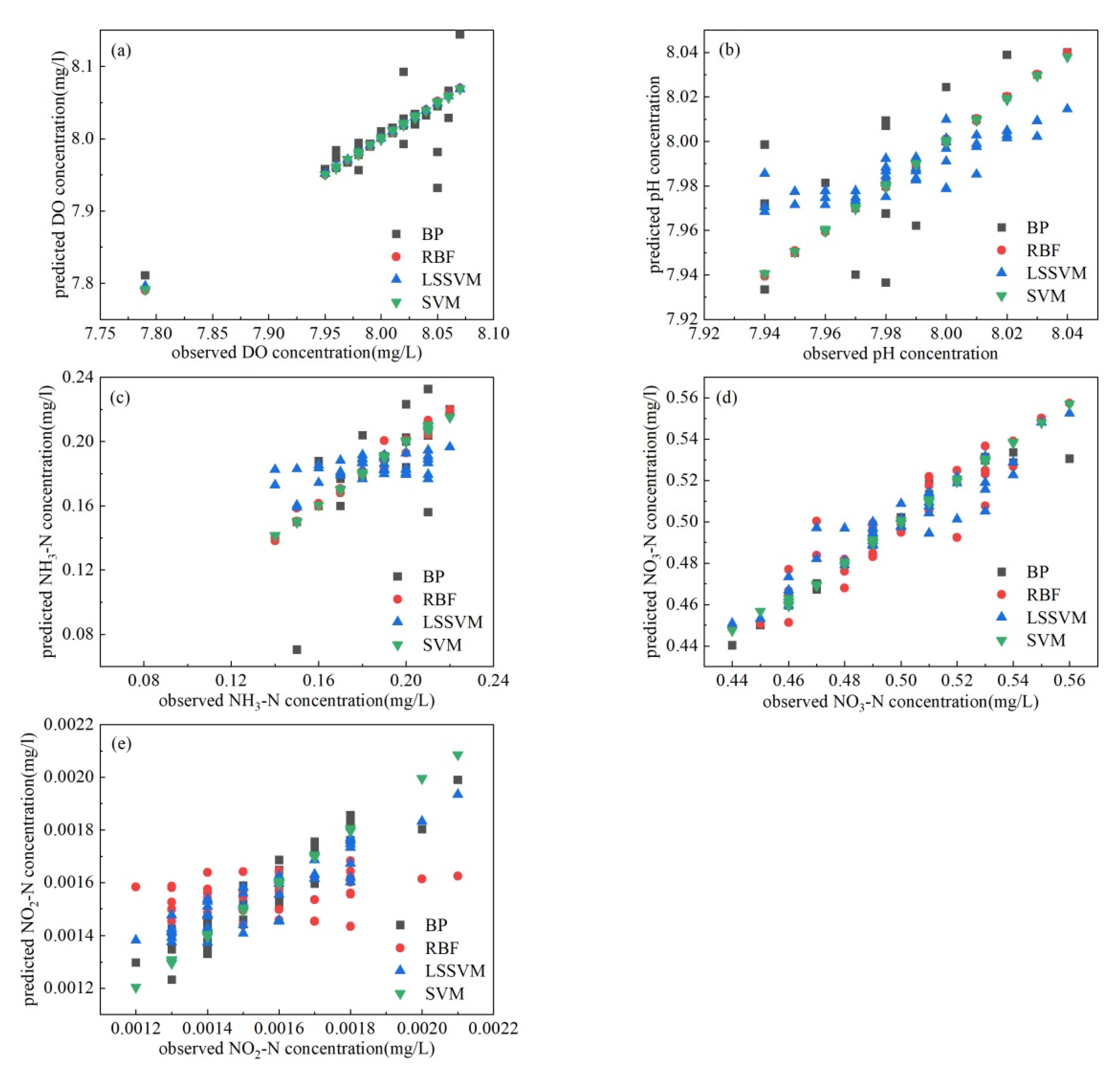
ANN is the preferred machine-learning model for predicting water quality because of its wide application area and good performance. However, ANN requires a large amount of data and is easy to fall into local minima. BPNN is a representative neural network of ANN with the disadvantage of falling into local minima. RBFNN has relatively stronger generalization ability than BPNN, so that this paper chose BPNN and RBFNN for the water quality prediction. SVM with strong approximation and generalization ability can overcome the problems that neural networks have difficulty avoiding. SVM has the disadvantage that SVM parameters determine the model performance. LSSVM can reduce the complexity of the algorithm on the basis of SVM. Therefore, SVM and LSSVM were chosen as complementary models for the water quality prediction. The published data were simulated and predicted using BPNN, RBFNN, SVM, and LSSVM (Figure 1).
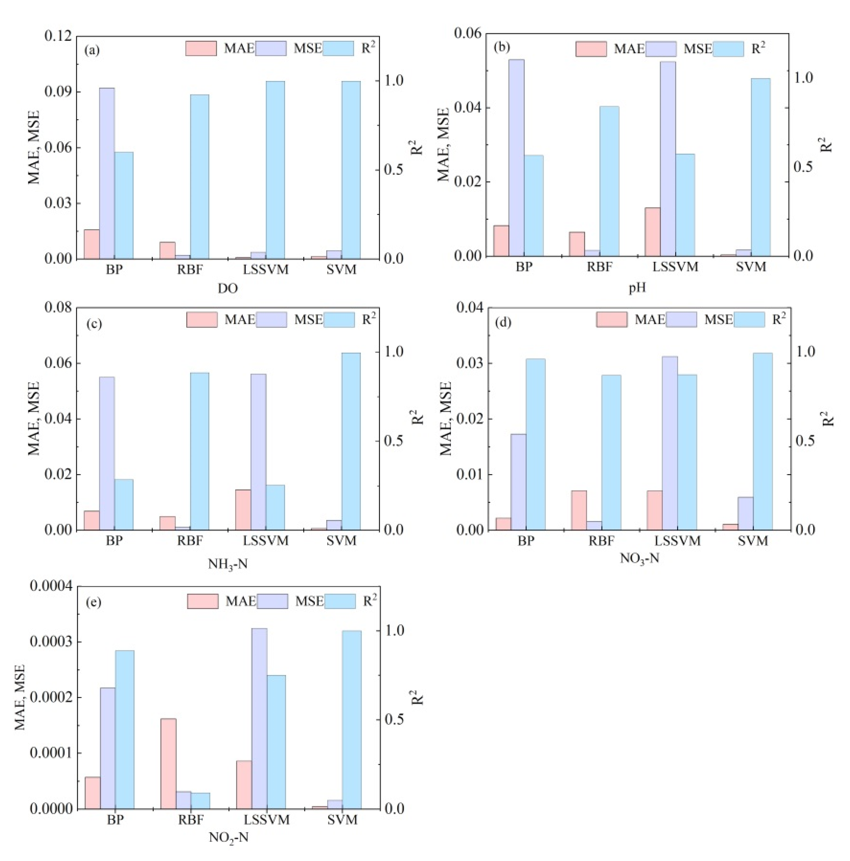
DO is an important factor in the growth and development of fish [32]. Figure 1a shows that the BPNN model was not as effective as the other three methods for predicting DO because its prediction results were less stable and the individual predicted values increased or decreased abnormally. The correlation coefficients of RBFNN, LSSVR, and SVR were as high as 0.999, while that for BPNN was only 0.6 according to the evaluation indexes in Figure 2a. The MAE and MSE of the BPNN were higher than those of the other three predictive models. Neural networks generally use the principle of empirical minimization when making predictions, which can easily fall into local optimization. SVM uses the principle of structural risk minimization so that the algorithm has global optimality, and the generalization ability of SVM is stronger than the neural network. Among the prediction results of the two neural networks, those for RBFNN were better than those for BPNN, which might be ascribed to the fact that RBFNN had stronger generalization ability than BPNN and RBFNN had the ability of global approximation to solve the problem of the local optimum of BPNN.
The pH is one of the key indicators in farmed water bodies to guide farmers in adjusting the production activities based on the indicators [33]. The prediction accuracy of BPNN and LSSVM was low, with correlation coefficients of 0.5 (Figure 1b). The MAE and MSE were 0.01 and 0.05, demonstrating that the prediction effects of both were not very good (Figure 2b). The prediction results for the SVM had a high degree of coincidence with the actual measured values with correlation coefficients as high as 0.999, while the MAE and MSE of SVM were 0.0004 and 0.002, respectively. The RBF neural network prediction was also good with a correlation coefficient of 0.80 and MAE/MSE of 0.007/0.002. The SVM predictions were more accurate than the other models.
The problem of high NH3-N concentration often occurs in breeding ponds, and excessive NH3-N will lead to decreased immunity, slow growth, poisoning, and the death of aquatic products. Therefore, it is important to predict NH3-N concentration to maintain the normal production of aquaculture. Figure 1c showed that SVM obtained the best prediction effect to match the measured value with the correlation coefficient of 0.996 and the MAE/MSE less than 0.001. The RBFNN prediction obtained the second best effect with a correlation coefficient of 0.88 and MAE/MSE of 0.005/0.001 (Figure 2c). The correlation coefficient of BPNN and LSSVM was less than 0.3, and the prediction effect was the worst.
NO3-N is another key indicator of water quality. Figure 1d showed that SVM obtained the best prediction effect among four models for NO3-N, followed by BPNN. The correlation coefficients of SVM/BPNN were 0.99/0.96, while MSE was 0.006/0.02 and MAE was 0.001/0.002 (Figure 2d). The correlation coefficients of both RBFNN and LSSVM prediction result was about 0.87 while the MSE and MAE were about 0.02 and 0.007, respectively.
Nitrite is converted into nitrate by nitrifying bacteria in an aerobic environment. Nitrate can be absorbed by aquatic plants and phytoplankton and converted into organic matter. It can also be converted into ammonia-nitrogen by denitrifying bacteria under anaerobic conditions. When the mass concentration of NO2-N in the water body is higher than 0.1 mg/L, it will endanger the normal growth of aquatic animals [34]. The best model and the worst model had a large gap in the predictions of nitrite-nitrogen (Figure 1e). SVM obtained the best prediction result with a correlation coefficient of 0.999, while RBFNN obtained the worst prediction effect with a correlation coefficient of only 0.08 (Figure 2e). The prediction effect of BPNN was second to LSSVM with a correlation coefficient of 0.88, while the prediction effect of LSSVM was second to that of BPNN with a correlation coefficient of 0.75.
The SVM model had the highest prediction accuracy and the best stability among the four models. Moreover, the data requirements of SVM were not strict to be suitable for aquaculture system with limited monitoring data. The accuracy of RBFNN in the prediction of individual indicators was also relatively high while its stability was not good with too large accuracy gap. Therefore, RBFNN was not suitable for the prediction of all indicators. The prediction results of BPNN and LSSVM were not good so that these two models were not considered for the following investigation.
3.2. Simulation and Prediction by Using Support Vector Machine
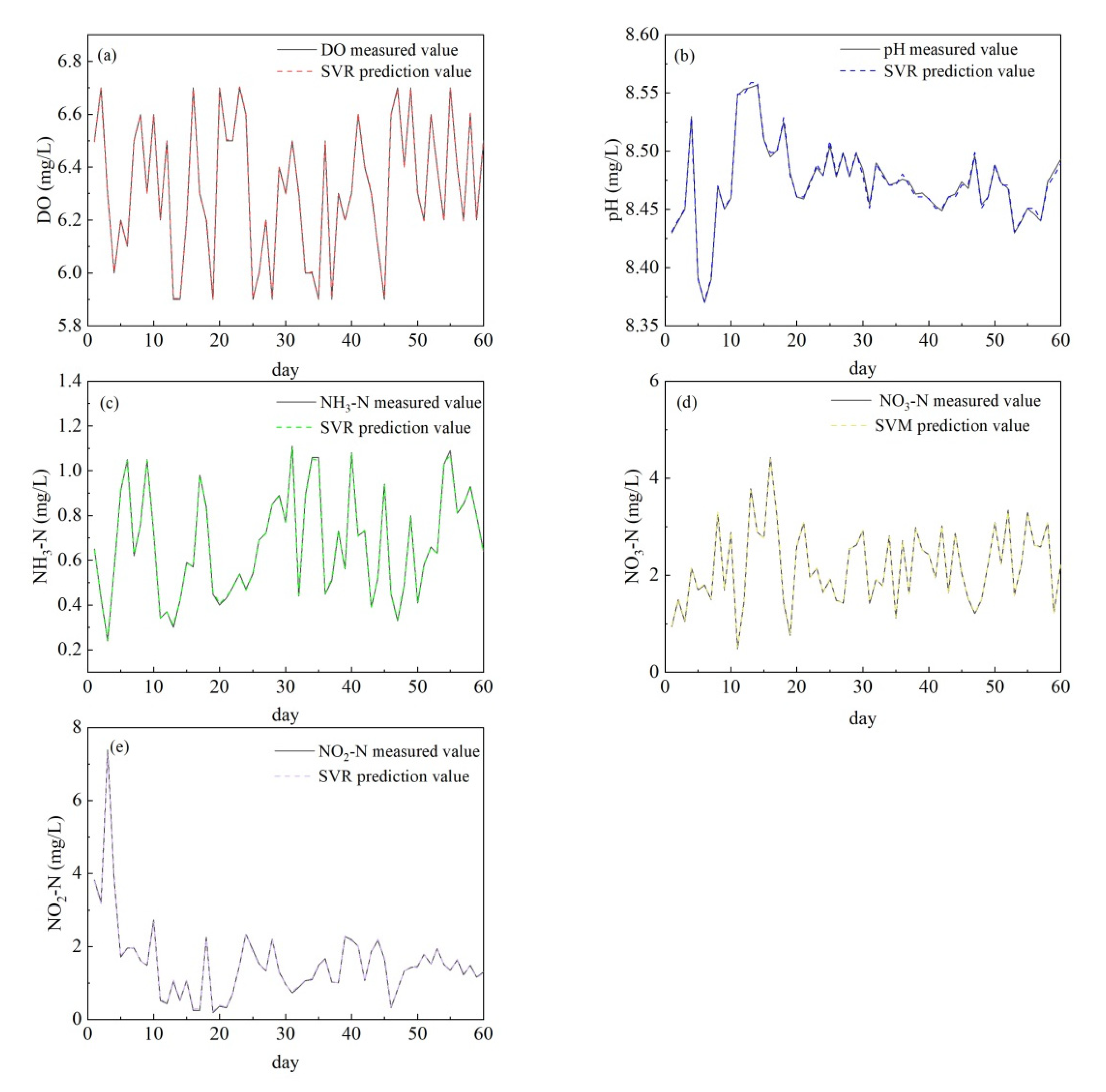
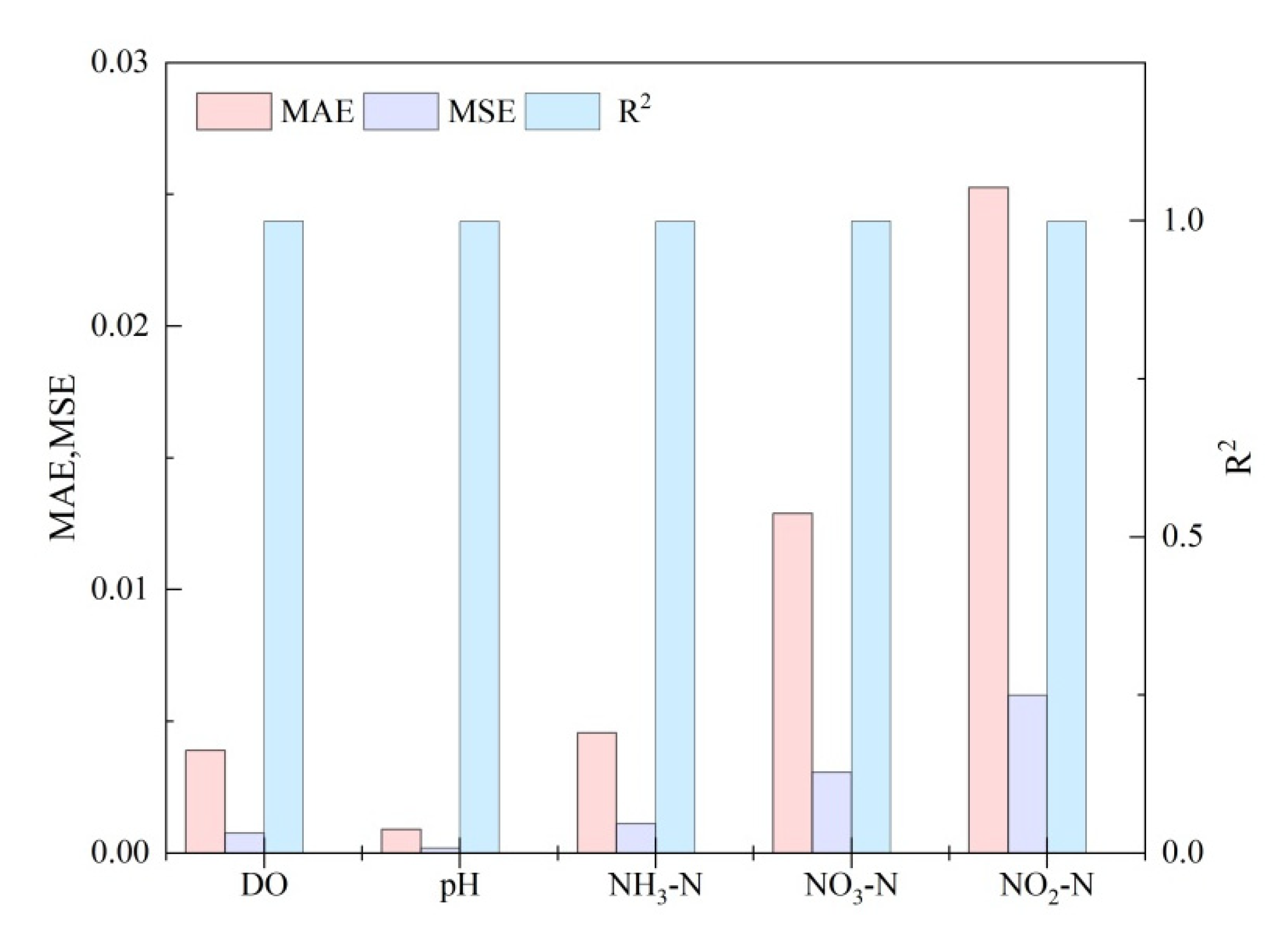
SVM illustrated excellent prediction ability for the published data. Thus, SVM was selected to predict the water quality data of the aquaculture body in an industrial aquaculture system. The prediction results are shown in Figure 3, and the performance indicators were also calculated (Figure 4).
The predicted values of five water quality parameters coincided well with the measured values to further prove the good prediction performance of the SVM model (Figure 3). The correlation coefficients were all as high as 0.999 (Figure 4 and Table 2). The MSE and MAE values of pH were the lowest, reaching 0.0002 and 0.001, respectively. The MSE and MAE of DO and ammonia-nitrogen were higher than those of pH and both lower than 0.01. The MSE and MAE of nitrate-nitrogen and nitrite-nitrogen were slightly higher, but both were lower than 0.05. The result showed that the prediction accuracy of SVM for measured data on industrial aquaculture water was still high, indicating that the prediction performance of SVM was excellent for application to actual prediction. SVM prediction will be beneficial to the monitoring and prognosis of industrial aquaculture systems. Moreover, short-term prediction is recommended for obtaining better prediction results.
Sensitivity analysis results showed that the model was more sensitive to pH when predicting DO parameters while the model was more sensitive to DO when predicting pH. Moreover, the model was more sensitive to NO3-N when predicting NH3-N while the model was more sensitive to NH3-N when predicting NO3-N. The model was more sensitive to NO3-N when predicting the NO2-N input.
SVM was the best prediction model for industrial aquaculture data among the four models. The SVM in this study also showed better prediction accuracy than methods reported previously. For example, the correlation coefficient of SVM prediction was 0.98 when predicting coastal ocean water quality [15] and 0.98 for groundwater level prediction [16]. SVM with 99% accuracy can be strongly recommended for water quality monitoring and prediction in industrial aquaculture. Parameter optimization can be carried out in order to obtain more accurate and stable prediction results.
The measured data for each parameter were interpolated to expand the data amount to reach 300. The expanded data were simulated and predicted using the SVM model (Figure 5). The results showed that the prediction accuracy of each parameter was higher than 95%. SVM was further confirmed to be a good model for predicting water quality in an industrial aquaculture system.
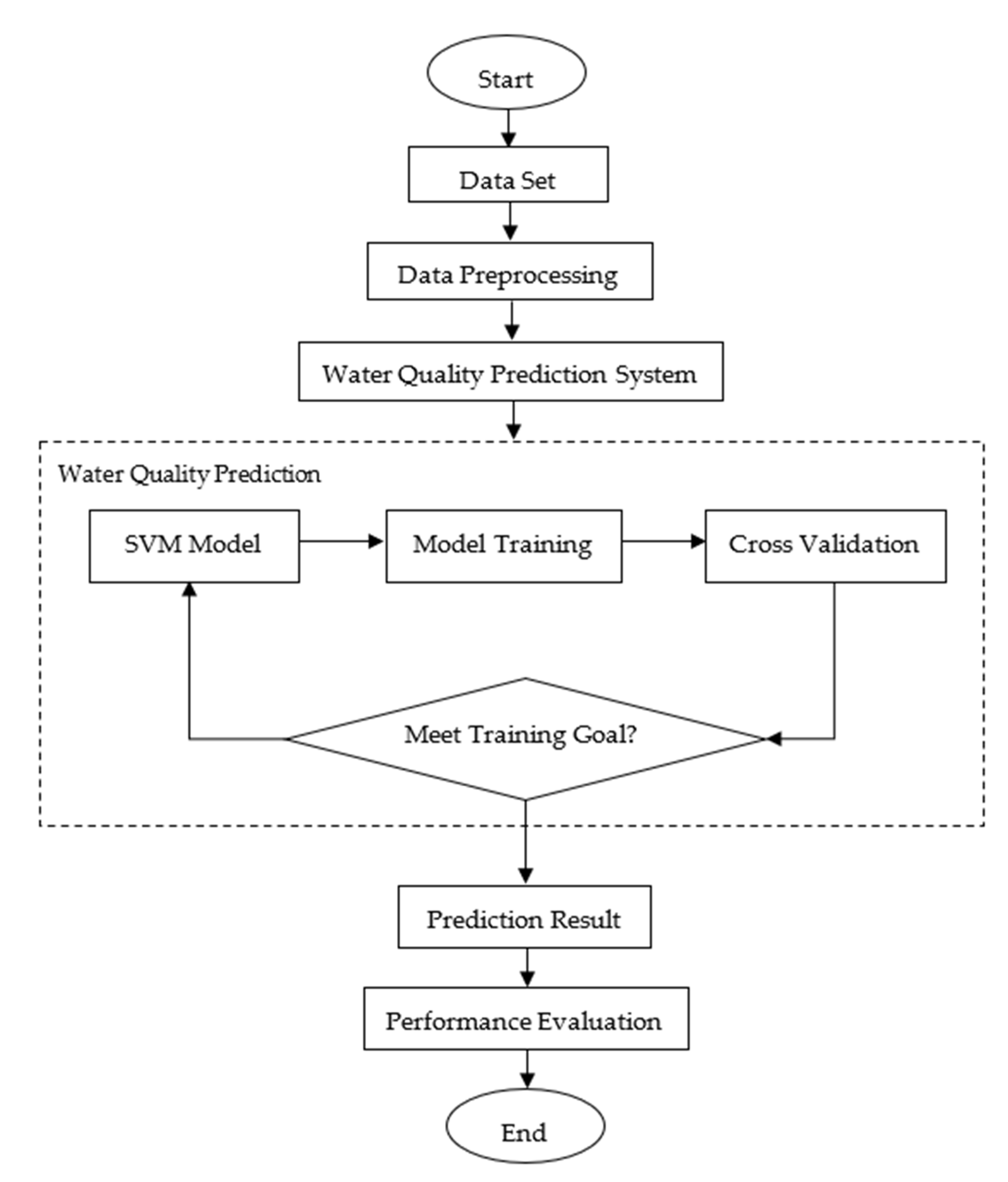
A water quality prediction system capable of predicting dissolved oxygen, ammonia-nitrogen, nitrate-nitrogen, pH, and nitrite-nitrogen is expected to be established. The specific flow chart is shown in Figure 6. The real-time water quality parameters are used as input, and then the prediction algorithm is used to predict the water quality data in the following days. Technical support for water quality prediction and early warning in actual production process are also needed. The cost of this system might be RMB 170,000 plus RMB 50,000 in annual maintenance fees.
4. Conclusions
This study used four machine learning models, BPNN, RBFNN, SVM and LSSVM, to simulate and predict five water quality parameters: DO, pH, NH4-N, NO3-N, and NO2-N. The major findings showed that SVM had better performance than the other three models with higher stability and lower data requirements. The accuracy of RBFNN in the prediction of individual indicators was also relatively high, but its stability was not high, and the accuracy gap was too large. The BPNN and LSSVM models were not suitable for predicting water quality parameters. It is feasible to use machine learning models to predict water quality in aquaculture systems. SVM showed excellent prediction performance for a real aquaculture farm. Shortcomings of the parameter selection of SVM occurred in this study. Parameter optimization methods can be used to obtain better prediction results. Water quality early warning can be added on the basis of water quality prediction for factory farming.
Author Contributions
Conceptualization, J.L.; methodology, T.L.; validation, L.C. and Z.Z.; resources, J.W.; writing—original draft preparation, T.L.; writing—review and editing, J.W. and J.L. All authors have read and agreed to the published version of the manuscript.
Funding
This research was funded by Youth Innovation Team Project for Talent Introduction and Cultivation in Universities of Shandong Province, the Taishan Scholars Program of Shandong Province (No. tsqn201812116), the Science and Technology Service Network Initiative of the Chinese Academy of Sciences (KFJ-STS-QYZX-114), and the Two-Hundred Talents Plan of Yantai.
Institutional Review Board Statement
Not applicable.
Informed Consent Statement
Not applicable.
Data Availability Statement
Not applicable.
Conflicts of Interest
The authors declare no conflict of interest.
References
- Lu, J.; Lin, Y.C.; Wu, J.; Zhang, C. Continental-scale spatial distribution, sources, and health risks of heavy metals in seafood: Challenge for the water-food-energy nexus sustainability in coastal regions? Environ. Sci. Pollut. Res. 2021, 28, 1–14. [Google Scholar] [CrossRef] [PubMed]
- Lu, J.; Wu, J.; Wang, J.H. Metagenomic analysis on resistance genes in water and microplastics from a mariculture system. Front Environ. Sci. Eng. 2022, 16, 4. [Google Scholar] [CrossRef]
- Lu, J.; Zhang, Y.X.; Wu, J.; Wang, J.H. Intervention of antimicrobial peptide usage on antimicrobial resistance in aquaculture. J. Hazard. Mater. 2022, 427, 128154. [Google Scholar] [CrossRef] [PubMed]
- Abdullah, A.H.; Saad, F.S.; Sudin, S.; Ahmad, Z.A.; Ahmad, I.; Abu, B.N.; Omar, S.; Sulaiman, S.F.; Che, M.H.; Umoruddin, N.A.; et al. Development of aquaculture water quality real-time monitoring using multi-sensory system and internet of things. J. Phys. Conf. Ser. 2021, 1, 2107. [Google Scholar] [CrossRef]
- Nguyen, X.C.; Nguyen, T.; La, D.D.; Kumar, G.; Nguyen, V.K. Development of machine learning—based models to forecast solid waste generation in residential areas: A case study from Vietnam. Resour. Conserv. Recycl. 2021, 167, 105381. [Google Scholar] [CrossRef]
- Rajaee, T.; Mirbagheri, S.A.; Zounemat-Kermani, M.; Nourani, V. Daily suspended sediment concentration simulation using ANN and neuro-fuzzy models. Sci. Total Environ. 2009, 407, 17. [Google Scholar] [CrossRef]
- Shouliang, H.; Zhuoshi, H.; Jing, S.; Beidou, X.; Chaowei, Z. Using Artificial Neural Network Models for Eutrophication Prediction. Procedia Environ. Sci. 2013, 18, 310–316. [Google Scholar]
- Chang, F.J.; Chen, P.A.; Chang, L.C.; Tsai, Y.H. Estimating spatio-temporal dynamics of stream total phosphate concentration by soft computing techniques. Sci. Total Environ. 2016, 562, 228–236. [Google Scholar] [CrossRef]
- Markus, M.; Tsai, C.W.S.; Demissie, M. Uncertainty of weekly nitrate-nitrogen forecasts using artificial neural networks. J. Environ. Eng. 2003, 129, 267–274. [Google Scholar] [CrossRef]
- Suen, J.P.; Eheart, J.W. Evaluation of neural networks for modeling nitrate concentrations in rivers. J. Water Resour. Plan. Manag. 2003, 129, 505–510. [Google Scholar] [CrossRef]
- Xu, X.; Sun, Z.J.; Wang, L.; Fu, J.; Wang, C. A Comparative Study of Customer Complaint Prediction Model of Time Series, Multiple Linear Regression and BP Neural Network. J. Phys. Conf. Ser. 2019, 1187, 052036. [Google Scholar] [CrossRef]
- Fan, Y.; Lu, W.X.; Miao, T.S.; An, Y.; Li, J.; Luo, J. Optimal design of groundwater pollution monitoring network based on the SVR surrogate model under uncertainty. Environ. Sci. Pollut. Res. Int. 2020, 27, 24090–24102. [Google Scholar] [CrossRef] [PubMed]
- Chia, S.L.; Chia, M.Y.; Koo, C.H.; Huang, Y.F. Integration of advanced optimization algorithms into least-square support vector machine (LSSVM) for water quality index prediction. Water Sci. Technol. Water Supply. 2022, 22, 1951–1963. [Google Scholar] [CrossRef]
- Kisi, O. Modeling discharge-suspended sediment relationship using least square support vector machine. J. Hydrol. 2012, 456, 110–120. [Google Scholar] [CrossRef]
- Deng, T.; Chau, K.W.; Duan, H.F. Machine learning based marine water quality prediction for coastal hydro-environment management. J. Environ. Manage. 2021, 284, 112051. [Google Scholar] [CrossRef]
- Mirarabi, A.; Nassery, H.R.; Nakhaei, M.; Adamowski, J.; Akbarzadeh, A.H.; Alijani, F. Evaluation of data-driven models (SVR and ANN) for groundwater-level prediction in confined and unconfined systems. Environ. Earth Sci. 2019, 78, 1–15. [Google Scholar] [CrossRef]
- Mirza, A.S.; Leal, J. Emulation of 2D Hydrodynamic Flood Simulations at Catchment Scale Using ANN and SVR. Water. 2021, 13, 2858. [Google Scholar] [CrossRef]
- Lu, H.; Ma, X. Hybrid decision tree-based machine learning models for short-term water quality prediction. Chemosphere 2020, 249, 126169. [Google Scholar] [CrossRef]
- Lnaa, B.; Jtb, B.; Taa, B. Ensemble method based on Artificial Neural Networks to estimate air pollution health risks—ScienceDirect. Environ. Model. Softw. 2020, 123, 104567. [Google Scholar]
- Li, J. Construction of legal incentive evaluation model based on BP neural network with multiple hidden layers. J. Phys. Conf. Ser. 2021, 1941, 012087. [Google Scholar] [CrossRef]
- Lourakis, M.I.A. A Brief Description of the Levenberg-Marquardt Algorithm Implemened by levmar. Found. Res. Technol. 2005, 4, 1–6. [Google Scholar]
- Kc, A.; Hc, B.; Cz, B. Comparative analysis of surface water quality prediction performance and identification of key water parameters using different machine learning models based on big data—ScienceDirect. Water Res. 2019, 171, 115454. [Google Scholar]
- Dandy, M. Neural networks for the prediction and forecasting of water resources variables: A review of modelling issues and applications. Environ. Model. Softw. 2000, 15, 101–124. [Google Scholar]
- Cherkassky, V.; Ma, Y. Practical selection of SVM parameters and noise estimation for SVM regression. Neural Netw. 2004, 17, 113–126. [Google Scholar] [CrossRef]
- Liu, X.P.; Lu, M.Z.; Chai, Y.Z.; Tang, J.; Gao, J.Y. A comprehensive framework for HSPF hydrological parameter sensitivity, optimization and uncertainty evaluation based on SVM surrogate model—A case study in Qinglong River watershed, China. Environ. Model Softw. 2021, 143, 150126. [Google Scholar]
- Leong, W.C.; Bahadori, A.; Zhang, J. Prediction of water quality index (WQI) using support vector machine (SVM) and least square-support vector machine (LS-SVM). Int. J. River Basin Manag. 2019, 19, 149–156. [Google Scholar] [CrossRef]
- Xu, W.; Wang, G.; Zhang, X. Prediction of Chlorophyll-a content using hybrid model of least squares support vector regression and radial basis function neural networks. In Proceedings of the 2016 Sixth International Conference on Information Science & Technology, Dalian, China, 6–8 May 2016. [Google Scholar]
- Del, G.D.; Muenich, R.L.; Kalcic, M.M. On the practical usefulness of least squares for assessing uncertainty in hydrologic and water quality predictions. Environ. Model Softw. 2018, 105, 286–295. [Google Scholar]
- Lei, T. Based on the Neural Network Model to Predict Water Quality; Haikou, D., Ed.; Hainan University: Haikou, China, 2015. [Google Scholar]
- Wang, S.; Yu, L.; Tang, L. A novel seasonal decomposition based least squares support vector regression ensemble learning approach for hydropower consumption forecasting in China. Energy 2011, 36, 6542–6554. [Google Scholar] [CrossRef]
- Sakaa, B.; Elbeltagi, A.; Boudibi, S.; Chaffaï, H.; Islam, A.R.M.T.; Kulimushi, L.C.; Choudhari, P.; Hani, A.; Brouziyne, Y.; Wong, Y.J. Water quality index modeling using random forest and improved SMO algorithm for support vector machine in Saf-Saf river basin. Environ. Sci. Pollut Res. Int. 2022, 29, 32. [Google Scholar]
- Cai, O.; Xiong, Y.; Yang, H. Phosphorus transformation under the influence of aluminum, organic carbon, and dissolved oxygen at the water-sediment interface: A simulative study. Front. Environ. Sci. Eng. 2020, 3, 165–176. [Google Scholar] [CrossRef]
- Iraní, S.M.; Vanessa, R.R.; Fernanda, L.A. The influence of the water pH on the sex ratio of tambaqui colossoma macropomum (CUVIER, 1818). Aquac. Rep. 2020, 17, 100334. [Google Scholar]
- Li, Y.; Ling, J.; Chen, P. Pseudomonas mendocina LYX: A novel aerobic bacterium with advantage of removing nitrate high effectively by assimilation and dissimilation simultaneously. Front. Environ. Sci. Eng. 2021, 15, 57. [Google Scholar] [CrossRef]
Figure 1.
The observed and simulated values of DO (a), pH (b), NH3-N (c), NO3-N (d), and NO2-N (e).

Figure 2.
Performance indicators including MAE and MSE of different algorithms. (a) DO; (b) pH; (c) NH3-N; (d) NO3-N; (e) NO2-N.
Figure 2.
Performance indicators including MAE and MSE of different algorithms. (a) DO; (b) pH; (c) NH3-N; (d) NO3-N; (e) NO2-N.

Figure 3.
Simulation and prediction of support vector machine on water body data of industrial aquaculture farm. (a) DO; (b) pH; (c) NH3-N; (d) NO3-N; (e) NO2-N.
Figure 3.
Simulation and prediction of support vector machine on water body data of industrial aquaculture farm. (a) DO; (b) pH; (c) NH3-N; (d) NO3-N; (e) NO2-N.

Figure 4.
Performance indicators of SVM algorithms.

Figure 5.
Simulation and prediction effect of support vector machine by using expanded data. (a) DO; (b) pH; (c) NH3-N; (d) NO3-N; (e) NO2-N.
Figure 5.
Simulation and prediction effect of support vector machine by using expanded data. (a) DO; (b) pH; (c) NH3-N; (d) NO3-N; (e) NO2-N.

Figure 6.
Prediction flow chart of water quality prediction system.


Table 1.
Measurement methods for each water quality parameter.
| Data | Measurement Methods |
|---|---|
| DO | DO sensor |
| pH | pH meter |
| NH3-N | Nessler’s reagent spectrophotometry |
| NO3-N | Ultraviolet spectrophotometric method |
| NO2-N | 1,2-diaminoethane dihydrochioride spectrophotometry |
Table 2.
Machine models predict the performance of water quality parameters.
| Published Data | Aquaculture Water Quality Data in Industrial Aquaculture Systems | ||||||
|---|---|---|---|---|---|---|---|
| Water Quality Parameter | Model | Result | Water Quality Parameter | Model | Result | ||
| MSE | R2 | MSE | R2 | ||||
| DO | BPNN | 0.092 | 0.60 | DO | SVM | 0.001 | 0.99 |
| RBFNN | 0.002 | 0.99 | |||||
| SVM | 0.003 | 0.99 | |||||
| LSSVM | 0.004 | 0.99 | |||||
| pH | BPNN | 0.053 | 0.56 | pH | SVM | 0.0002 | 0.99 |
| RBFNN | 0.002 | 0.84 | |||||
| SVM | 0.002 | 0.99 | |||||
| LSSVM | 0.052 | 0.57 | |||||
| NH3-N | BPNN | 0.055 | 0.28 | NH3-N | SVM | 0.001 | 0.99 |
| RBFNN | 0.001 | 0.88 | |||||
| SVM | 0.004 | 0.99 | |||||
| LSSVM | 0.056 | 0.25 | |||||
| NO3-N | BPNN | 0.017 | 0.96 | NO3-N | SVM | 0.003 | 0.99 |
| RBFNN | 0.002 | 0.87 | |||||
| SVM | 0.006 | 0.99 | |||||
| LSSVM | 0.031 | 0.87 | |||||
| NO2-N | BPNN | 0.002 | 0.87 | NO2-N | SVM | 0.006 | 0.99 |
| RBFNN | 0.351 | 0.08 | |||||
| SVM | 0.001 | 0.99 | |||||
| LSSVM | 0.064 | 0.75 | |||||
Publisher’s Note: MDPI stays neutral with regard to jurisdictional claims in published maps and institutional affiliations. |
© 2022 by the authors. Licensee MDPI, Basel, Switzerland. This article is an open access article distributed under the terms and conditions of the Creative Commons Attribution (CC BY) license (https://creativecommons.org/licenses/by/4.0/).
Share and Cite
MDPI and ACS Style
Li, T.; Lu, J.; Wu, J.; Zhang, Z.; Chen, L. Predicting Aquaculture Water Quality Using Machine Learning Approaches. Water 2022, 14, 2836. https://doi.org/10.3390/w14182836
AMA Style
Li T, Lu J, Wu J, Zhang Z, Chen L. Predicting Aquaculture Water Quality Using Machine Learning Approaches. Water. 2022; 14(18):2836. https://doi.org/10.3390/w14182836
Chicago/Turabian StyleLi, Tingting, Jian Lu, Jun Wu, Zhenhua Zhang, and Liwei Chen. 2022. "Predicting Aquaculture Water Quality Using Machine Learning Approaches" Water 14, no. 18: 2836. https://doi.org/10.3390/w14182836
Note that from the first issue of 2016, this journal uses article numbers instead of page numbers. See further details here.