

On the Shift of Glacier Equilibrium Line Altitude (ELA) under the Changing Climate
Institute for Atmospheric and Climate Science (IAC), Swiss Federal Institute of Technology (E.T.H.), Universitätstrasse 16, CH-8092 Zurich, Switzerland
*
Author to whom correspondence should be addressed.
Water 2022, 14(18), 2821; https://doi.org/10.3390/w14182821
Submission received: 25 May 2022
/
Revised: 29 August 2022
/
Accepted: 7 September 2022
/
Published: 10 September 2022
(This article belongs to the Special Issue Review and Progress in Hydrological and Meteorological Monitoring of Glaciers)
Abstract
:Presently available information on the glacier equilibrium line altitude (ELA) is being collected and examined. The historical course of the world’s longest ELA series of 107 years at the Claridenfirn is reviewed together with climatic elements. Further, the changes in ELAs of 70 glaciers the world over are investigated, and a linear plane model for the speed of the ELA shift is proposed as a function of the changing rates of summer temperature and winter mass balance. The four glaciers in Europe, which diverge most from the plane, are investigated in detail. The cause of the divergence is likely due to be the change in solar global radiation. Although a precise quantification of the role of radiation is not possible at this stage for the entire world, the role of solar radiation is investigated for these glaciers. Globally viewed, ten, or 15% of the 70 investigated glaciers, are expected to lose their accumulation areas within the next ten years. Half of all studied glaciers will follow the same fate by the end of this century under the present climatic conditions. If climate change is accelerated, the disappearance of glaciers will occur sooner than presented in this study.
1. Introduction
The glacier equilibrium line separates the accumulation and ablation areas. In detail, the separation may not appear in one line on the glacier surface. It may appear as a zone in which accumulation and ablation patches intermingle. The equilibrium line often appears at different altitudes on the same glacier, especially on its east and west sides. The equilibrium line altitude is its average altitude. The average altitudinal belt of such a transition zone is usually narrow, which justifies the concept of the equilibrium line altitude, often abbreviated as ELA. By definition, the annual net mass balance (Bn) on the ELA is zero. In the literature, the ELA has often been referred to as a snow line. A historical survey on the development of the concept of the ELA was recently made by Braithwaite [1]. The ELAs on many glaciers are presently rapidly shifting worldwide, but the shifting speed varies with a wide range. Few works that are concerned with mass balance and ELA have investigated their relation to climate change [2]. This article is especially aimed at presenting the relationship between the ELA shift and climatic elements.
The ELA is a convenient concept, as it is directly related to the climate on the glacier. The ELA and the annual net mass balance (Bn) are closely related to most glaciers. The ELA is also indicative of the water discharge from the glacierized drainage basin. Further, an ELA can be estimated by visual observations at the end of the summer on glaciers with an insignificant superimposed ice formation. Further, ELAs have the advantage of relating glacier change to climate change in a simple manner, in comparison with elaborated distributed balance methods [3].
From several hundred glaciers with mass balance and ELA observations, 70 glaciers were chosen with a view to the quality and duration of the observations. In the following sections, the status of the current ELA variations will be reviewed. First, the variations of the world’s longest record of the mass balance, hence ELA on the Claridenfirn, in the European Alps, are presented, followed by the used material for the paper. A special emphasis was given to detecting and correcting reported glaciological data. Then, the processes of the ELA shift will be statistically analyzed. The statistically presented ELA variations are physically interpreted based on the energy balance of the ELA. Finally, the changing rates of the ELAs will be summarized as a function of widely available climatic elements.
2. Overview of the ELA Variations
2.1. The Longest Observation of the ELA
The longest measurement of mass balance, hence the ELA, in the world started in the summer of 1914 on the Claridenfirn in the Glarneralpen near the northern fringe of the Swiss Alps. At present, the glacier has a surface area of about 5 km2, stretching from 2540 to 3240 m a.s.l. with a median altitude of about 2860 m a.s.l. The average ELA of the last 107 years is 2805 m a.s.l. The accumulation area has a rare extensive flat and near-horizontal surface. The initial motivation for the twice-annual measurements of the winter (Bw) and summer mass balance (Bs) was more for meteorology than glaciology. The initiators of the self-financed project were meteorologists at the Swiss Meteorological Central Office, who were aware of the significantly different precipitation at high altitudes in comparison with that at lower altitudes, where most observations were carried out. Their idea was to regard the accumulation area of the Claridenfirn as a gigantic snow gauge [4]. The twice-annual mass balance measurement has continued until today without a break. A detailed account of the mass balance of the Claridenfirn was recently summarized [4]. The present subsection augments this work [4] with more climatological considerations.
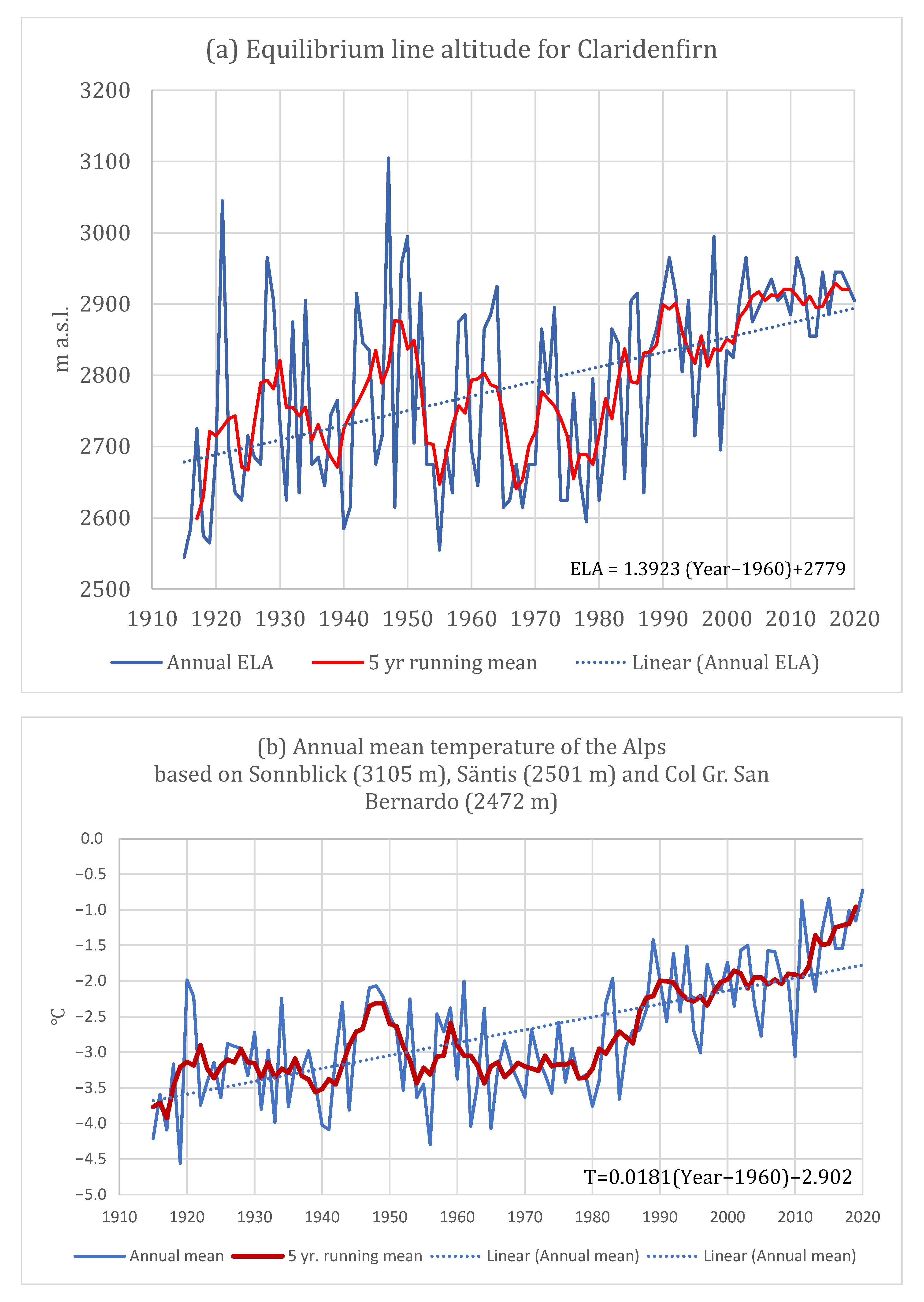
Three plots are presented in Figure 1. Figure 1a illustrates the annual ELA from the 1914/1915 to 2017/2018 mass balance years. A curve representing the 5-year running mean is added. The mean ELA of the observation period was 2805 m with a standard deviation of 125 m. A quick visual examination of the figure together with the following Figure 1b,c shows that the high and low ELAs are closely related to climatic elements, especially air temperature and precipitation. For example, high ELA years, such as 1921, 1928, 1947, and 1998, are all associated with the peaks of high summer temperatures and lower precipitation. On the other hand, the low ELAs between 1940 and 1984 are seen together with low summer temperatures and high precipitation. Further, during a quarter century from the 1950s to the 1980s, the ELA frequently descended by 200 m below the average. This phase of lower ELA, corresponding to the 30-year cooling period (cf. Figure 1b) in the middle of the otherwise warming century, was a global phenomenon and often overlooked due to a preoccupation with the century of climate warming. In addition to these decadal fluctuations, there is a clear ascending tendency of ELA on a century scale. The annual ascending rate of 1.4 m a−1 makes a total ascent of 150 m during the last 107 years, which lies clearly outside the standard deviation of 125 m. In the next section, the ELA variations of the glaciers in other regions of the world will be presented.
2.2. ELA Changes on Observed Glaciers World Over
In the next step, 70 glaciers with long-term mass balance observations were globally chosen and presented in Supplementary Materials. In this table, the annual ELAs are presented for each glacier. The ELAs in red are estimated values with the correlation regression lines based on the ELA and annual net balance (Bn) relationship, which will later be explained in detail. The following last seven lines at the bottom of the table provide: (1) the mean ELA for each glacier; (2) the vertical displacement of ELA during the 40 years from 1979 to 2018 in m; (3) the standard deviation of annual ELA; (4) ELAs as its linear regression line cuts the year 2020; (5) the maximum altitude of the glacier; (6) the annual rate of the ELA shift in ma−1; (7) the year after 2020, estimated for the glacier to lose the accumulation area. The glaciers without accumulation areas are called terminal glaciers and are doomed to disappear in due time. The number of terminal glaciers is increasing worldwide, owing to the current warming. Of the 70 glaciers in this table, 11%, or 8, glaciers will lose their accumulation areas before 2030, and 50% of the glaciers will follow the same process by the end of this century.
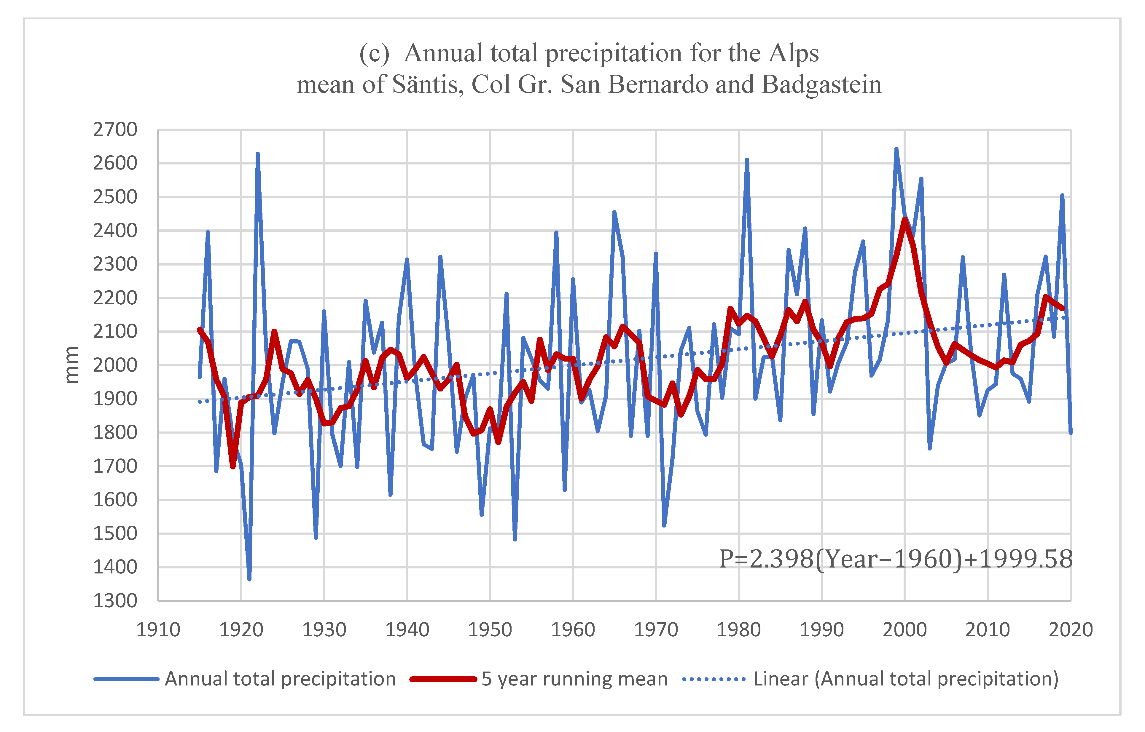
After excluding several glaciers whose observation periods were too short, the remaining glaciers were grouped into 17 regions, and their mean ELA histories are presented in Figure 2. The common periods of observation are the last half century leading to 2020. No glaciers were chosen from the Equatorial and Tropic regions due to frequently missing observations. Nevertheless, one can see that the common range of the regional shift of the ELAs falls between 2 and 5 ma−1, with extremes at 8 ma−1 in Kamchatka and −5 ma−1 in the Antarctic. The ELAs are rising in all regions, except for the Antarctic. The wide range of the regional ELA shift is recognizable. The range of the ELA for each glacier is much larger, as presented in Supplementary Materials. The prime objective of the present work is to understand this wide range of variation from a systematic viewpoint.
3. The Data Sources and Their Treatment
3.1. Publications and On-Line Accessible Data Files
The present study required a substantial amount of glaciological and climatic data. The data had to be homogenous and long enough to recognize the changes in ELAs and climatic elements, that is, at least 30 years, and if possible, longer. Glaciological data used in the present work were based on the open data files maintained by the World Glacier Monitoring Service (WGMS) in two files, Overview, and Mass Balance, and many national and private information sources. This rather elaborate data collection was necessary, as the information in one source could be plagued by errors and missing information, as will be discussed later in the next subsection. All national and private publications/sources are presented in Appendix A, and only the essential and most-used sources are presented in the following text. Among the national data sources, the following were essential for this paper: Glaciological Investigations in Norway (1963–2020); die Gletscherberichte (later under Die Gletscher der Schweizer Alpen, and further, Schnee, Gletscher und Permafrost) (1880–2020); Summaries of many years’ observations, such as for glaciers on Axel Heiberg Island [5], Arctic [6], Austria [7,8,9], Scandinavia [10], and the ex-Soviet Union [11]. The information on the same subjects and for the same glaciers is often different. In such cases, the most recent information is used. As the stake measurements are becoming more adjusted by geodetic information, the authors trust the most recent information after the reevaluation, as recommended by Andreassen et al. [12].
Meteorological and climatological data are internationally more coordinated and accessible than glaciological information. Basic meteorological and climatological information, such as the long-term temperature and precipitation, is available in such collections as CRUTEM (University of East Anglia) and GHCN (Global Historical Climatology Network). For the Alpine region, HISTALP (Historical Instrumental Climatological Surface Time Series of the Greater Alpine Region) [13] plays an important role. The temperature is usually taken from the ERA5 Reanalysis [14]. The period of ERA5 completed by the time of the preparation of this paper was forty years from 1979 to 2018, which was adopted for this paper. The ERA5 data has been interpolated to a 0.25° longitude by 0.25° latitude grid. The summer (JJA in the Northern and DJF in the Southern Hemisphere) mean temperature values are linearly interpolated from the horizontally surrounding grid points onto the position of each glacier. In the vertical, the temperature value of the first model level above the model’s boundary layer height in the free atmosphere is taken to avoid uncertainties from parameterizations of the boundary layer processes over the complex topography. It is nevertheless essential to consult the direct observations, especially when ERA5 obviously fails. Most frequently consulted are the National Meteorological and Geophysical Service of Austria (Zentral Anstalt für Meteorologie und Geodynamik), the Swiss Federal Office for Meteorology and Climatology (MeteoSwiss), Norwegian Meteorological Institute, the Swedish Meteorological and Hydrological Institute, and the German Weather Service. Radiation data were obtained from the WRDC (World Radiation Data Centre, Sankt Petersburg), GEBA (Global Energy Balance Archive, Zurich) [15], and BSRN (Baseline Surface Radiation Network, Bremerhaven) [16].
3.2. Examination and Construction of the ELA Timeseries
Most data sources with information on ELA are not suitable for use in their original form. ELAs are often missing in the reports, or not observable when the entire glacier surface becomes the ablation area, or in rare cases, the accumulation area. There are several possible options to supplement the reported ELAs as follows: (1) do nothing to alter the reported ELA, including missing or unobserved years; (2) correct obvious errors, but leave the rest as reported. The altitude for “>maximum glacier altitude” will be set for this maximum altitude by ignoring “>“; (3) supplement missing years, for example, by a correlation between the ELA and Bn.
Option (1) causes grave problems as there are so many errors in the mass balance and ELA reports, including the WGMS files, as an example will be shown later in this subsection. Option (2) is definitely an improvement over Option (1) but leaves the problem of the “ELA disappearance” above the glacier. Without these years, the trend and the mean ELA will be biased for lower ELA. Option (3) appears reasonable but causes an additional problem. First, the estimated ELA “above the glacier” cases calculated by the correlation of ELA and Bn often yield lower ELAs than the maximum height of the glacier. The reason is that the majority of cases lie below the maximum glacier altitude. Hence, the extrapolated hypothetical ELA above the glacier tends to be pulled down, even below the maximum glacier surface altitude. Further, such an extrapolation is risky because it introduces an artificial treatment to observed data.
We will show these problems with a case found in a report of the South Cascade Glacier in the North Cascades in the State of Washington, U.S.A. The South Cascade Glacier is one of the benchmark glaciers and is reported by the U.S.G.S. (United States Geological Survey) [17]. It is a small valley glacier with a length of 2.1 km and a surface area of 1.8 km2 (2015), facing north-west. The lowest surface is the glacier front at 1620 m a.s.l. The highest margin of the glacier lies at 2275 m a.s.l, according to the WGMS. The highest topographic surface of the drainage basin is Sentinel Peak at 2518 m a.s.l. The mass balance measurement started in 1953 and is one of the longest glacier monitoring works in North America. The mass balance of this glacier is reported to WGMS in Zurich and also to NSIDC (National Snow and Ice Data Center) in Boulder, Colorado. Table 1 shows the most up-to-date versions of the mass balance and ELA available from the WGMS. The table was made by merging the ELA and the mass balance data from WGMS-FoG-2021-05-E-MASS-BALANCE_OVERVIEW, and WGMS-FoG-2021-05-EE-MASS-BALANCE, respectively.
The ELA of the year 1966 is reported as 2380 m a.s.l., while the upper margin of the glacier is 2275 m, which is impossible. Furthermore, it is unlikely that the ELA lies above the glacier, as the Bw and Bs for 1966 are near average for this glacier. Ten years later, the ELA of 1977 was reported as “>2250”, which is below the glacier’s maximum altitude. Four years later, in 1980, the ELA was reported as “>2150”. The upper margin of the glacier would have had to sink by 100 m in a short time. This is extremely unlikely. Then, for the following five years from 1981 to 1985, ELAs are missing, although Bw, Bs, and Bn are reported. These years were not extreme enough to expect the ELA to be soaring above the glacier or lying below the glacier snout. Three years later, in 1988, the ELA was again missing, although Bw, Bs, and Bn are reported. In later years, the highest glacier surface to lose the ELA was variously reported as, for example, 2244 m, 2125 m, 2317 m, 2754 m, and 2331 m. The glacier’s upper boundary could indeed change from year to year, but 2125 m is well below the glacier’s maximum altitude, and 2317 m and 2331 m are clearly off the official maximum height of 2275 m. The ELA for 2002 in the WGMS file is 1856, while the USGS report gives 1820 m [17]. These are minor problems. By the time when the year 2019 is reached and one finds the ELA as “>3264 m”, one realizes this is clearly wrong, as the highest ground surface in the drainage basin is 2518 m a.s.l. (Sentinel Peak).
These problems are not uncommon in glaciological data but are becoming increasingly important as more ELAs are climbing above the maximum glacier surface in recent years. To calculate the trend, one needs accurate data. If all doubtful data are eliminated for further analyses, the researchers would be confronted with an insufficient data quantity, which makes the application of statistics difficult. Consequently, for the present work, the missing ELAs are estimated with Bn, choosing Option (3) presented in the first paragraph of the present subsection. There are the following three options for applying this method: (a) ELA/Bn correlation excluding the years of “>maximum altitude”; (b) the correlation will be calculated by setting “>maximum altitude” to the maximum altitude, and (c) the same as Option (a), but only with data of the negative mass balance years. From various trial and error attempts, Option (c) gave the most realistic result and was used in the present work. The ELA/Bn correlative diagram has non-linearity. By eliminating the data from the positive balance years from the calculation of the regression line, one can circumvent the complications of the non-linear regression line. The elimination of the pair ELA and Bn of the positive mass balance year can be justified as the ELA of the positive balance tends to lie in the long-term ablation area where the surface gradient tends to be steeper than the upper accumulation area, causing non-linearity in the ELA/Bn curve.
In rare cases, there are some glaciers where the entire glacier surface becomes the accumulation area. The hypothetical ELA must lie below the glacier front. In this case, strong snow drift tends to be involved, by creating an unduly high accumulation in the lower part of the glacier. This case is more difficult to deal with in comparison with the cases of the ELA disappearing above the glacier. Since the problem of snow drift is beyond the scope of the present paper, and since these cases are extremely rare, the ELAs of such years are set to the minimum altitude of the glacier. After supplementing the ELA for the missing years as explained above, the annual ELAs for the 70 glaciers are presented in the table in Appendix A. The estimated ELAs are indicated in red figures.
Glaciers with less than 50% of the useful ELA during the entire observing period, such as Fontana Bianca and Careser, are excluded from further analysis.
4. The Climatology of the Equilibrium Line Shift
4.1. Search for the Universal Relationship between the ELA Shift and Climate Change
As the main objective of the present article is to find causes for the ELA shift, 53 glaciers were selected for further analysis with respect to the duration of mass balance observations, the availability of the winter and summer balances, and the meteorological stations within short distances. The main characteristics attributed to these glaciers are presented in Table 2. Two glaciers in South America and a glacier in Africa were added to the table, although they do not satisfy the above-mentioned condition of the choice. Hence, they were not used for the present analysis, but the available information attributed to them could help readers in their future works.
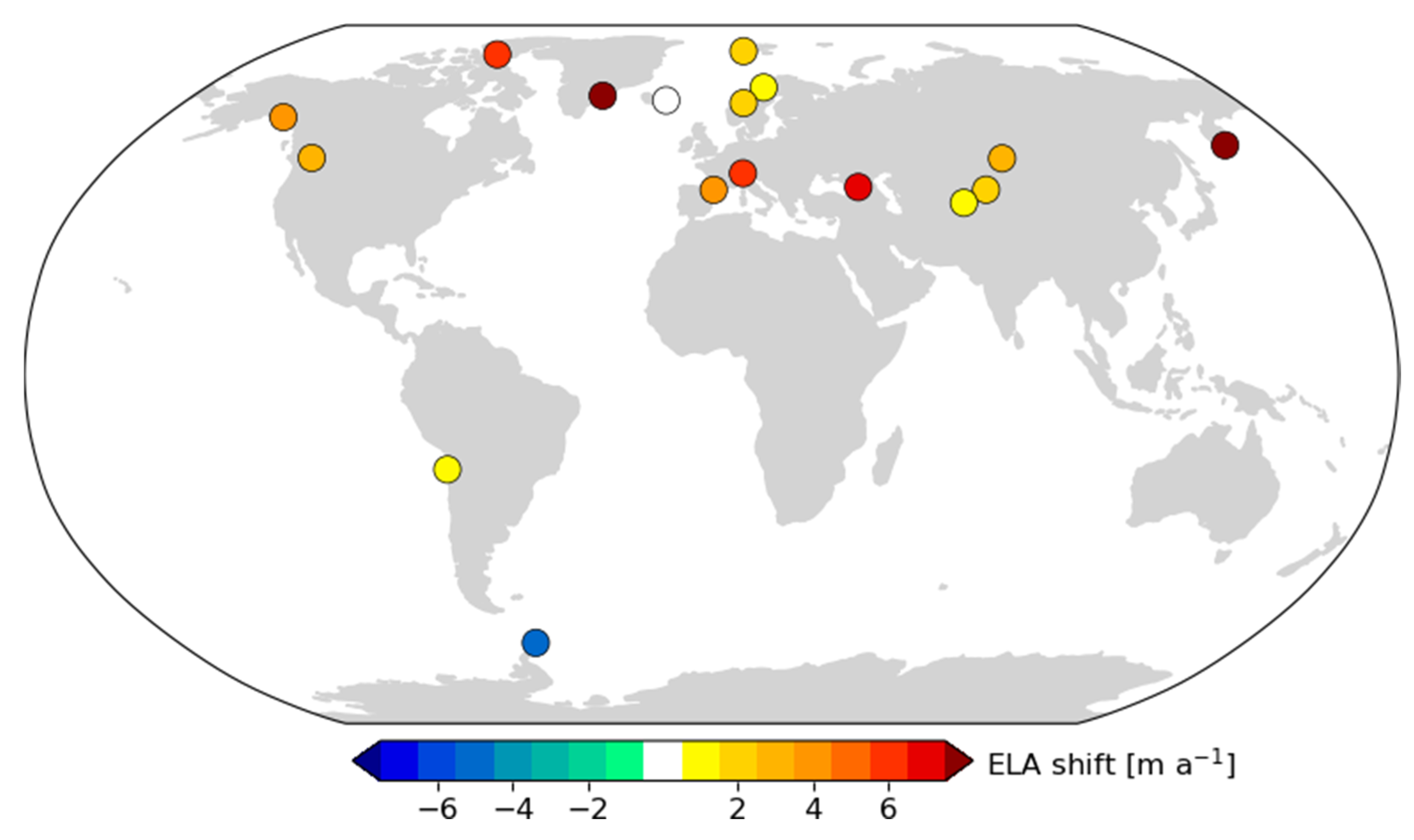
In Figure 3, the annual rates of the ELA shift are compared with the decadal summer temperature changes. In general, one sees a positive correlation between the shifting speed of the ELA (ma−1) and the rate of temperature change (K/decade). The sector for the cooling temperature shows a good correlation with the sinking rate of the ELA, but the sector for the rising temperature is occupied with glaciers with a wide range of ELA shifts. Furthermore, the accumulation represented by the winter balance, Bw was investigated. The numbers assigned to each dot represent the rates (mm w.e. a−1) of the winter mass balance change (Bw). Ideally, this variable should be the annual accumulation, but such an observation is not available for most glaciers. The fact that the winter balance represents a good portion of the annual accumulation was presented for a number of glaciers [18]. However, on glaciers in the interior of the continents, such as the Tienshan Mountains, the winter is dormant, and most accumulation and ablation happen simultaneously in summer. For such glaciers, the rates of the winter balance change were substituted with the rates of the annual precipitation change at nearby meteorological stations.
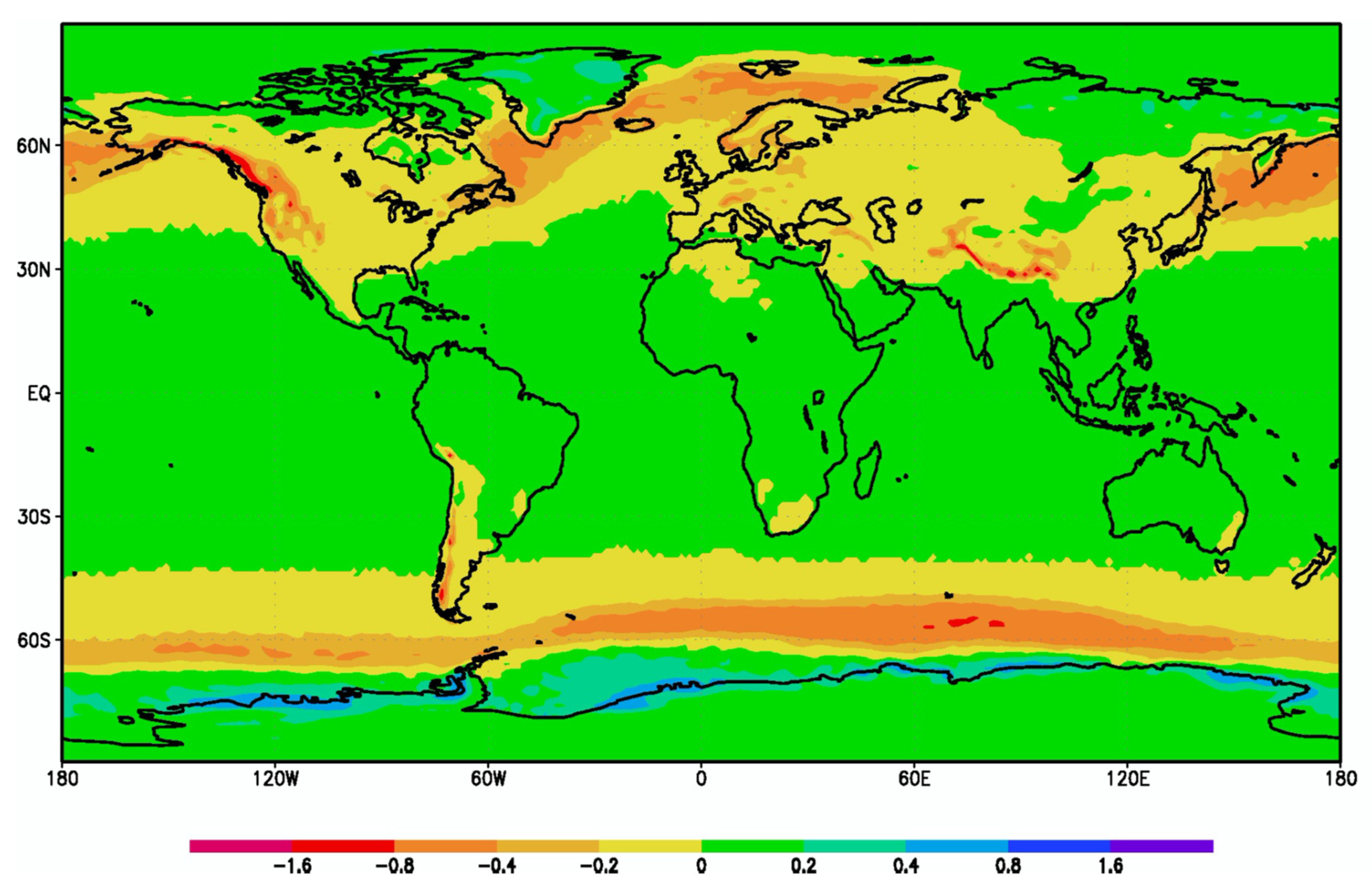
The fastest ELA rise under an insignificantly small temperature increase is represented by the Lemon Creek Glacier in Alaska. This glacier is located in a maritime climatic region with the high precipitation of the northwest coast of North America. The region has been showing a strong decrease in observed precipitation, which is also reflected in a strong negative trend of Bw of the Lemon Creek Glacier. The authors studied the present trend of the observed precipitation in this region. Prince Rupert and Dawson in Canada, and Sitka in the USA, Alaska are the only three stations with long observations with few missing observations. The trends in the observed annual total precipitation for the period from 1979 to 2018 are −41.3 mm/a, −1.21, and −6.7, respectively. This tendency coincides with the result of the high-resolution GCM experiment, based on ECHAM5 with T106 resolution, which shows that the Alaskan Panhandle will become the fastest precipitation-losing region in the world (Figure 4). In the report by Vicente-Serrano et al. [19], ECHAM5 belonged to a minority that reported decreasing precipitation for this area, while the majority produced increasing precipitation. This situation clearly shows the fact that many models that participated in the Coupled Model Intercomparison Project (CMIP) failed in simulating precipitation.
Another glacier with the fastest ELA rise is Basodino, a valley glacier in the Alps. This glacier indicates no change in Bw but is located on the southern fringe of the Alps, where one of the fastest temperature increases, T, has been observed. Therefore, in these glaciers, one sees two main components that influence the shift of ELA, Bw, and T. The general trend that Bw and T determined the geographical distribution of ELA to a great extent was empirically found by Ahlmann [20] and theoretically supported by Ohmura and Boettcher [21]. The present analysis also shows that these two factors, Bw and T, are important for determining the changing speed of the ELAs with respect to time.
Based on the above information, one can conceive of a three-dimensional space occupied by the rates of ELA shift (E), temperature change (T), and the winter balance shift (Bw). As an approximation, the following first-order regression plane can be considered:
where, a and b are coefficients that must be determined by the observed E (ma−1), T (K/decade), and Bw (mma−1). The third term on the right side, “c” represents a possible contribution made by variables other than T and Bw, and the error.
E = a T + b Bw + c,
The least-square regression analysis provides the following results: a = 6.39, b = −0.15, and c = 1.55. The 95% confidence intervals are (4.74; 8.05), (−0.236; −0.057), and (0.78; 2.33), respectively. R2 is 0.60. The projection of this plane onto the E/T plane at Bw = 0 is also plotted in Figure 3.
4.2. Significance of Equation (1), Physical Content of c, and the Situation of Outliers
Equation (1) allows estimating the shifting speed of an ELA given a set of climatic information on the rates of temperature change and winter accumulation or annual precipitation. It also gives a weight of each factor for causing the ELA shift as follows: 1 K/decade, or 0.1 Ka−1 temperature change T, would cause an ELA shift of 6.4 ma−1. To cause the same ELA shift, Bw alone would need to change by 43 mma−1. The temperature 1 K equivalence in the ELA shift is 430 mm of solid precipitation in water equivalent (w.e.). This value can be compared with earlier publications with 1 K/350 mm expected on an ELA [18]. Recently, Braithwaite and Hughes [22] proposed a 1 K temperature sensitivity (probably synonymous with equivalence) from 0.4 to 1 m, a considerably higher value.
There are four glaciers that deviate grossly from the trend expressed in Equation (1). They are Hintereisferner in Austria, Griesgletscher, and Basodino in Switzerland, and Hofsjokull E in Iceland. The first two glaciers are in Figure 3, in the neighborhood of decreasing and no change in Bw, while the actual Bw on these glaciers is rapidly increasing. The third mentioned, Basodino, is also located in the region of strong Bw decrease, but the observed Bw change is practically zero. Hofsjokull E, on the other hand, has a fast-decreasing Bw, yet the ELA ascent is much slower than the general trend might indicate. These deviations are probably due to the influence of the long-term change in solar global radiation (the sum of direct and diffuse solar radiation), which has so far not been taken into account [23]. Solar global radiation in Europe has been generally increasing during the last forty years [24]. Based on the best 12 stations with radiometry in Europe, the mean annual change in solar global radiation is estimated at 0.29 Wm−2/a for the period from 1979 to 2018. There are four stations in the eastern Alpine region, where Griesgletscher, Basodino, and Hintereisferner are located, and high-quality observations of radiation are maintained. They are Jungfraujoch, Grimselhospiz, Säntis, and Innsbruck. The mean increasing rate of the solar global radiation at these sites is 0.62 Wm−2/a, which is more than double the average increasing rate in Europe.
The situation on the Hofsjokull E is the exact opposite of the three Alpine glaciers discussed above. Hofsjokull E has been the only Icelandic glacier with both winter and summer balance measurements lasting for more than 30 years. Despite the large loss of the Bw at a rate of 10 mm/a, the ascending rate of the ELA remained only at 1 ma−1. The solar global radiation measured at nearby Reykjavik shows a distinctly different course in comparison with the rest of Europe. Namely, solar radiation has been decreasing throughout the observation period of the last 60 years. The change in the period from 1979 to 2018, which is adopted as the period of detailed study in this article, is −0.16 Wm−2/a, in comparison with the mean European rate of +0.29 Wm−2/a. It appears that the role of solar radiation is not unimportant.
An independent proof for this hypothesis can be seen in eight glaciers in southern Norway, south of 62° N. These glaciers are all clustered around the two regression lines of Figure 3 with an almost constant Bw changing rate of about −6 mm/a, with the exceptions of Austdalsbreen and Nigardsbreen (Alfot −9 mma−1, Hanse −4, Gråsu −6, Hellstungu −6, Stor −7 and Hardanger −5). The radiometric station at Bergen shows an extremely steady condition of solar global radiation, both in terms of summer and the annual total.
Based on this analysis, the authors consider that a substantial portion of the term “c” in Equation (1) must be due to the change in solar global radiation. A statistical evaluation of the global influence of the solar radiation shift is not possible at this stage, as long-term high-quality radiation measurements near the glaciers are rare. However, the search for a better fitting location for the four outliers in the ELA/Temperature diagram of Figure 3 can be used to estimate the influence of the change in solar radiation. The best material is from Basodino, where Bw remained practically unchanged at 0. This glacier should be found on the regression lines in Figure 3. However, the (T, E) for the Basodino is shifted far to the left, as the temperature change, T is only 0.57 K/decade. If we assume that the point should have been on the regression line, which stands for a Bw = 0 situation, the difference in T must be +0.63 K/decade. If this difference in the energy source was provided by the increase in solar radiation of the same period, 0.63 K/decade should be equivalent to 0.62 Wm−2/a. This consideration leads to a mutual equivalence of 1 K change to 430 mm of ice in water equivalent (w.e.), and 9.8 Wm−2 for solar radiation. This analysis suggests that the last term of the constant in the equation, 1.55, can be replaced by 0.65 R, where R is the rate of the change in solar global radiation in a year, Wm−2/a. A previous analysis for establishing the ELA resulted in values of 1 K corresponding to 350 mm of ice in w.e., and 7 Wm−2 of solar radiation, respectively [18]. One thus concludes that the change in solar radiation also has a significant role in shifting the glacier equilibrium line. Earlier, 1 K temperature equivalence from 0.4 to 1 m (w.e.) of ice accumulation by Braithwaite and Hughes [22] was quoted. These higher values are probably due to the exclusion of the contribution from solar radiation. In their consideration, the contribution from solar radiation is included in the accumulation change. Therefore, the actual equivalence by temperature alone must inevitably be smaller than from 0.4 to 1 m (w.e.) of ice melting.
5. Results and Conclusions
Glacier equilibrium line altitude (ELA) is a good indicator of the glacier mass balance. ELA is especially suited to characterize the reaction of a glacier to a changing climate. An example was presented for correcting the errors that are common in reported glaciological data, including ELAs. The shift of the ELA is globally investigated, and the process of the shift is analyzed. By studying the equilibrium lines on 70 glaciers, it was found that on 60 glaciers the ELAs are ascending, leaving 10 glaciers where the ELAs are descending. Common ascending rates of ELA fall between 2 and 5 ma−1. The strongest ascending speed of about 10 ma−1 is reported for the Lemon Creek Glacier in the Alaskan Panhandle and the Basodino on the southern edge of the Swiss Alps. All reported glaciers in the Antarctic showed descending ELAs. Globally viewed, ten, or 15% of the 70 investigated glaciers, are expected to lose their accumulation areas within the next ten years. Half of all studied glaciers will follow the same fate by the end of this century under the present climatic conditions. The ELAs’ shifting speed (E) is statistically analyzed and found to fit to the regression plane of E = 6.39 T − 0.15 Bw + 1.55, with R2 = 0.6, where the units for E, T, and Bw are [m/a], [K/decade], and [mm w.e./a], respectively. Further, the changing rate of solar global radiation was found to play a role that should be considered in future studies. The limited case study with the Southern Alps of Europe suggests the last term of the constant in the equation, 1.55, can be replaced by 0.65 R, where R is the rate of the change in solar global radiation in Wm−2/a. The present investigation suggests that the change of solar radiation by 9.8 Wm−2 causes the shift of the ELA equivalent to a 1 K temperature change or a 430 mm accumulation change.
Supplementary Materials
The following supporting information can be downloaded at: https://www.mdpi.com/article/10.3390/w14182821/s1, Table S1: Equilibrium line altitude of selected glaciers and their main characteristics. The last seven lines at the bottom of the table provide, (1): mean ELA for each glacier, (2): the vertical displacement of ELA during 40 year from 1979 to 2018 in m, (3): the standard deviation of annual ELA, (4): ELAs as its linear regression line cut the year 2020, (5): maximum altitude of the glacier, (6): annual rate of the ELA shift in ma−1, and (7): the year after 2020, esti-mated for the glacier to lose the accumulation area. Bold figures represent regional values. Figures in red are estimated values based on the ELA and Bn relationship as explained in the text. Blanks are missing information.
Author Contributions
A.O. worked on the glaciological side of the article, while M.B. contributed on the meteorological aspects, especially concerning with GCMs and the Re-Analysis. All authors have read and agreed to the published version of the manuscript.
Funding
The present work was supported by the budget of the Institute for Atmospheric and Climate Science, E.T.H., where the first author continues working after the formal retirement in 2007.
Acknowledgments
The authors are indebted to the two anonymous reviewers who provided valuable comments for the first manuscript. The authors thank Tamaki Ohmura at the Swiss Federal Institute for Forest Snow and Landscape Research WSL, who assisted the authors for the statistical calculations in this article.
Conflicts of Interest
The authors declare no conflict of interest.
Appendix A
Data and material sources used in the article:
- WGMS-FoG-2021-05-E-MASS-BALANCE_OVERVIEW, and WGMS-FoG-2021-05-EE-MASS-BALANCE, World Glacier Monitoring Service (WGMS), Zurich
- Glaciological Investigations in Norway (1963-2020), Norwegian Water Resources and Energy Directorate
- Gletscherberichte (later under Die Gletscher der Schweizer Alpen, and further, Schnee, Gletscher und Permafrost) (1880-2020), Glacier Commission, Swiss Academy of Natural Sciences
- Baker, E. H., McNeil, C. J., Sass, L. C., Peitzsch, E. H., Whorton, E. N., Florentine, C. E., Clark, A. M., Miller, Z. S., Fagre, D. B., and O’Neel, S., 2018, USGS Benchmark Glacier Mass Balance and Project Data: U.S. Geological Survey data release, https://doi.org/10.5066/F7BG2N8R.
- McNeil, C. J., Sass, L. C., Florentine, C. E., Baker, E. H., Peitzsch, E. H., Whorton, E. N., Miller, Z. S., Fagre, D. B., Clark, A. M., and O’Neel, S., 2016, Glacier-Wide Mass Balance and Compiled Data Inputs: USGS Benchmark Glaciers: U.S. Geological Survey data release, https://doi.org/10.5066/F7HD7SRF.
- ERA5 reanalysis
- CRUTEM (Climate Research Unit, University of East Anglia)
- GHCN (Global Historical Climatology Network). For the Alpine region
- HISTALP (Historial Instrumental Climatological Surface Time Series of the Greater Alpine Region)
- National Meteorological and Geophysical Service of Austria (Zentral Anstalt für Meteorologie und Geodynamik)
- Swiss Federal Office for Meteorology and Climatology (MeteoSwiss)
- German Weather Service
- Canadian Meteorological Service
- Swedish Meteorological and Hydrological Institute
- Norwegian Meteorological Institute
- Bergen radiation reports, Geophysical Institute, University of Bergen
- WRDC (World Radiation Data Centre, Sankt Petersburg)
- GEBA (Global Energy Balance Archive, ETH, Zurich)
- BSRN (Baseline Surface Radiation Network, AWI, Bremerhaven)
References
- Braithwaite, R.J. From Doctor Kurowski’s Schneegrenze to our modern glacier equilibrium line altitude (ELA). Cryosphere 2015, 9, 2135–2148. [Google Scholar] [CrossRef]
- Rutgers, F. Bericht der Gletscher-Kommission der Physikalischen Gesellschaft Zürich. Polarforschung 1914, 36, 75–76. [Google Scholar]
- Hock, R. Temperature index melt modelling in mountain area. J. Hydrol. 2003, 282, 104–115. [Google Scholar] [CrossRef]
- Huss, M.; Bauder, A.; Linsbauer, A.; Gabbi, J.; Kappenberger, G.; Steinegger, U.; Farinotti, D. More than a century of direct glacier mass-balance observations on Claridenfirn, Switzerland. J. Glaciol. 2021, 67, 697–713. [Google Scholar] [CrossRef]
- Cogley, J.G.; Adams, W.P.; Ecclestone, M.A.; Jung-Rothenhäusler, F.; Ommanney, C.S.L. Mass balance of Axel Heiberg Island Glaciers 1960–1991. NHRI Sci. Rep. 1995, 6, 168. [Google Scholar]
- Johansson, M. Mass Balance Data from Arctic Glaciers; IASC working Group for Arctic Glaciers, IASC: Geneva, Switzerland, 2002; 20p. [Google Scholar]
- Kuhn, M.; Kaser, G.; Markl, G.; Wagner, H.P.; Schneider, H. 25 Jahre Massenhaushaltsuntersuchungen am Hintereisferner; Institute of Meteorology and Geophysics, University of Innsbruck: Innsbruck, Austria, 1979; 80p. [Google Scholar]
- Kuhn, M.; Abermann, J.; Bacher, M.; Olefs, M. Transfer of mass-balance profiles to unmeasured glaciers. Ann. Glaciol. 2009, 50, 185–190. [Google Scholar] [CrossRef]
- Lambrecht, A.; Kuhn, M. Glacier changes in the Austrian Alps during the last three decades, derived from the new Austrian glacier inventory. Ann. Glaciol. 2007, 46, 177–184. [Google Scholar] [CrossRef]
- Holmlund, P.; Jansson, P.; Pettersson, R. A re-analysis of the 58 year mass-balance record of Storglaciären, Sweden. Ann. Glaciol. 2005, 42, 489–495. [Google Scholar] [CrossRef]
- Dyurgerov, M. Mass Balance Monitoring of Mountain Glaciers; Nauka: Moscow, Russia, 1993; 125p. (In Russian) [Google Scholar]
- Andreassen, L.M.; Elvehøy, H.; Kjøllmoen, B.; Belart, J.M.C. Glacier change in Norway since 1960s—an overview of mass balance, area, length and surface elvation changes. J. Glaciol. 2020, 66, 313–328. [Google Scholar] [CrossRef]
- Auer, I.; Reinhard, B.; Anita, J.; Wolfgang, L.; Alexander, O.; Roland, P.; Wolfgang, S.; Markus, U.; Christoph, M.; Keith, B. HISTALP-historical instrumental climatological surface time series of the Greater Alpine Regions. Int. J. Climatol. A J. R. Meteorol. Soc. 2007, 27, 17–46. [Google Scholar] [CrossRef]
- Hans, H.; Bill, B.; Paul, B.; Shoji, H.; András, H.; Joaquín, M.-S.; Julien, N.; Carole, P.; Raluca, R.; Dinand, S. The ERA5 global reanalysis. Q. J. R. Meteorol. Soc. 2020, 146, 1999–2049. [Google Scholar] [CrossRef]
- Wild, M.; Ohmura, A.; Schär, C.; Müller, G.; Folini, D.; Schwarz, M.; Hakuba, M.Z.; Sanches-Lorenzo, A. The Global Energy Balance Archive (GEBA) version 2017: A database for worldwide measured surface energy fluxes. Earth Syst. Sci. Data 2017, 9, 601–613. [Google Scholar] [CrossRef] [Green Version]
- Amelie, D.; John, A.; Klaus, B.; Sergio, C.; Christopher, C.; Emilio, C.-A.; Fred, M.D.; Thierry, D.; Masato, F.; Hannes, G. Baseline Surface Radiation Network (BSRN): Structure and data description (1992-2017). Earth Syst. Sci. Data 2018, 10, 1491–1501. [Google Scholar]
- Bidlake, W.R.; Josberger, E.G.; Savoca, M.E. Water, Ice, and Meteorological Measurements at South Cascade Glacier, Washington, Balance Year 2003; Scientific Investigations Report 2005-5210; U.S. Geological Survey: Reston, VA, USA, 2005; p. 48. [Google Scholar]
- Ohmura, A.; Kasser, P.; Funk, M. Climate at the equilibrium line of glaciers. J. Glaciol. 1992, 38, 397–411. [Google Scholar] [CrossRef]
- Vicente-Serrano, S.M.; García-Herrera, R.; Peña-Angulo, D.; Tomas-Burguera, M.; Domínguez-Castro, F.; Noguera, I.; Calvo, N.; Murphy, C.; Nieto, R.; Gimeno, L.; et al. Do CMIP models capture long-term observed annual precipitation trends? Clim. Dyn. 2022, 58, 2825–2842. [Google Scholar] [CrossRef]
- Ahlmann, H.W.S. Le niveau de glaciation comme function de l’accumulation d’humidité sous forme solide. Méthode pour le calcul de l’humidité condensée dans la haute montagne et pour l’étude de la fréquence des glaciers. Geografiska Annaler 1924, 6, 223–272. [Google Scholar]
- Ohmura, A.; Boettcher, M. Climate on the equilibrium line altitudes of glaciers: Theoretical background behind Ahlmann’s P/T diagram. J. Glaciol. 2018, 64, 489–505. [Google Scholar] [CrossRef]
- Braithwaite, R.J.; Hughes, P.D. Positive degree-day sums in the Alps: A direct link between glacier melt and international climate policy. J. Glaciol. 2022, 2022, 1–11. [Google Scholar] [CrossRef]
- Ohmura, A.; Bauder, A.; Müller, H.; Kappenberger, G. Longterm change of mass balance and the role of radiation. Ann. Glaciol. 2007, 46, 1–8. [Google Scholar] [CrossRef]
- Wild, M. Decadal changes in radiative fluxes at land and ocean surfaces and their relevance for global warming. Wiley Interdiscip. Rev. Clim. Chang. 2016, 7, 91–107. [Google Scholar] [CrossRef]
Figure 1.
The equilibrium line altitude (ELA) of the Claridenfirn and the climatic condition: (a) Annual ELA from 1915 to 2018; (b) Summer mean temperature (JJA) of the Alps, based on Sonnblick (3105 m), Säntis (2501 m) and Col Gr. San Bernardo (2472 m); (c) Annual total precipitation for Alps, mean of Säntis, Col Gr. San Bernardo and Badgastein (1094 m). The thick red lines are 5-year running means, while the dotted lines are linear regression lines from 1915 to 2020. The equations for the regression lines are provided at the right-bottom corners.


Figure 2.
Regional mean shift of the ELA for 70 glaciers in 17 geographical regions. In 16 cases the ELAs showed ascent with varying rates. In only one region, the Antarctic, the ELAs descended. The ELA-related information for each glacier is given in Supplementary Materials.
Figure 2.
Regional mean shift of the ELA for 70 glaciers in 17 geographical regions. In 16 cases the ELAs showed ascent with varying rates. In only one region, the Antarctic, the ELAs descended. The ELA-related information for each glacier is given in Supplementary Materials.

Figure 3.
The relationship between the ELA shift rate (m/a) and the decadal temperature change (K/decade). Each dot represents a glacier with accompanying number representing the annual change in Bw (mm/a). The changing rate of the winter balance (Bw) marked in red represents the glaciers discussed in the text (from top left, Lemon Creek, Basodino, Hintereis, Gries, and Hofs E). The dot-line is the best fit regression line on the E/T plane. The solid straight line is the interseption of the best fit plane discussed in the text with the Bw = 0 plane. The proximity of these two lines indicates a good accuracy of the plane.

Figure 4.
The change in annual solid precipitation expected in the last three decades of this century, computed with ECHAM5 T106 under the IPCC Scenario A2 (scale at the bottom is in mmd−1). Note that he northwest of North America is forecast to lose 500–600 mma−1 precipitation.
Figure 4.
The change in annual solid precipitation expected in the last three decades of this century, computed with ECHAM5 T106 under the IPCC Scenario A2 (scale at the bottom is in mmd−1). Note that he northwest of North America is forecast to lose 500–600 mma−1 precipitation.


Table 1.
Annual mass balance for the South Cascade Glacier as stored at WGMS: last three columns present the results of the ELA estimations from left with all pairs of ELA (m a.s.l.) and Bn (mm w.e.), excluding the pairs for ELA above the glacier, and the last column, with ELA and Bn with only negative Bn.
| Year | Bw (mm) | Bs (mm) | Bn (mm) | Off Glacier | Reported | With All Data | Excluding Above | Only Negative |
|---|---|---|---|---|---|---|---|---|
| ELA m a.s.l. | glacier ELA | Bn years | ||||||
| 1953 | −600 | |||||||
| 1955 | 300 | |||||||
| 1956 | 200 | |||||||
| 1957 | −200 | |||||||
| 1958 | −3300 | |||||||
| 1959 | 3290 | −2560 | 730 | |||||
| 1960 | 2220 | −2690 | −470 | 1880 | ||||
| 1961 | 2410 | −3480 | −1070 | 1950 | ||||
| 1962 | 2510 | −2280 | 230 | 1860 | ||||
| 1963 | 2240 | −3510 | −1270 | 2040 | ||||
| 1964 | 3260 | −2030 | 1230 | 1795 | ||||
| 1965 | 3490 | −3630 | −140 | 1880 | ||||
| 1966 | 2480 | −3480 | −1000 | 2380 | 2009 | 2043 | 2034 | |
| 1967 | 3300 | −3900 | −600 | 1870 | ||||
| 1968 | 3010 | −2970 | 40 | 2080 | ||||
| 1969 | 3180 | −3880 | −700 | 1910 | ||||
| 1970 | 2420 | −3590 | −1170 | 2050 | ||||
| 1971 | 3520 | −2890 | 630 | 1820 | ||||
| 1972 | 4280 | −2820 | 1460 | 1770 | ||||
| 1973 | 2220 | −3230 | −1010 | 2070 | ||||
| 1974 | 3660 | −2610 | 1050 | 1850 | ||||
| 1975 | 3070 | −3090 | −20 | 1800 | ||||
| 1976 | 3540 | −2560 | 980 | 1825 | ||||
| 1977 | 1580 | −2850 | −1270 | > | 2250 | 2036 | 2076 | 2076 |
| 1978 | 2500 | −2850 | −350 | 1925 | ||||
| 1979 | 2190 | −3720 | −1530 | 2225 | ||||
| 1980 | 1840 | −2830 | −990 | > | 2150 | 2008 | 2041 | 2033 |
| 1981 | 2290 | −3100 | −810 | 1990 | 2019 | 2005 | ||
| 1982 | 3120 | −3010 | 110 | 1896 | 1905 | 1862 | ||
| 1983 | 1920 | −2660 | −740 | 1982 | 2010 | 1994 | ||
| 1984 | 2390 | −2240 | 150 | 1892 | 1900 | 1856 | ||
| 1985 | 2190 | −3360 | −1170 | 2026 | 2064 | 2061 | ||
| 1986 | 2480 | −3340 | −860 | 1995 | ||||
| 1987 | 1960 | −4050 | −2090 | 2189 | ||||
| 1988 | 2210 | −3400 | −1190 | 2028 | 2066 | 2064 | ||
| 1989 | 2400 | −3590 | −1190 | 2024 | ||||
| 1990 | 2530 | −2880 | −350 | 1889 | ||||
| 1991 | 3650 | −4020 | −370 | 1883 | ||||
| 1992 | 1850 | −4050 | −2200 | 2080 | ||||
| 1993 | 1880 | −2920 | −1040 | 1991 | ||||
| 1994 | 2350 | −4120 | −1770 | > | 2244 | 2087 | 2138 | 2153 |
| 1995 | 2980 | −4000 | −1020 | 1997 | ||||
| 1996 | 2860 | −2970 | −110 | 1868 | ||||
| 1997 | 3470 | −3140 | 330 | 1835 | ||||
| 1998 | 3070 | −4950 | −1880 | > | 2137 | 2098 | 2152 | 2170 |
| 1999 | 4040 | −2480 | 1560 | 1847 | ||||
| 2000 | 3110 | −2580 | 530 | 1840 | ||||
| 2001 | 1760 | −2550 | −790 | 1966 | ||||
| 2002 | 3990 | −3400 | 590 | 1856 | ||||
| 2003 | 2460 | −4690 | −2230 | > | 2125 | 2133 | 2195 | 2225 |
| 2004 | 2060 | −3660 | −1600 | 2108 | ||||
| 2005 | 2090 | −4470 | −2380 | > | 2317 | 2149 | 2214 | 2248 |
| 2006 | 2600 | −3830 | −1230 | > | 2754 | 2032 | 2071 | 2070 |
| 2007 | 3490 | −3470 | 20 | 1869 | ||||
| 2008 | 3280 | −3120 | 160 | 1850 | ||||
| 2009 | 2730 | −4380 | −1650 | > | 2331 | 2075 | 2123 | 2135 |
| 2010 | 2700 | −2930 | −230 | 1907 | ||||
| 2011 | 3550 | −2150 | 1400 | 1794 | ||||
| 2012 | 3530 | −3430 | 100 | 1854 | ||||
| 2013 | 3280 | −3940 | −660 | 1915 | ||||
| 2014 | 3710 | −3840 | −130 | 1926 | ||||
| 2015 | 2730 | −5950 | −3220 | 2174 | ||||
| 2016 | 3410 | −4170 | −760 | 1963 | ||||
| 2017 | 3960 | −4570 | −610 | 1941 | ||||
| 2018 | 3800 | −4480 | −680 | 2040 | ||||
| 2019 | 2440 | −4490 | −2050 | > | 3264 | 2115 | 2173 | 2197 |
| 2020 | 3210 | −3270 | −60 | 1885 |
Table 2.
The rates of changes: ELA shift (ma−1), temperature (K/decade), and winter balance (mma−1).
Table 2.
The rates of changes: ELA shift (ma−1), temperature (K/decade), and winter balance (mma−1).
| Glacier | Latitude | Longitude | Mean ELA m a.s.l. | Observed Period | Used Period | ELA Change m/a | Temp Change K/Decade | Bw Change mm w.e./a | Comments | Meteorol. Stations Used |
|---|---|---|---|---|---|---|---|---|---|---|
| Canadian Arctic | ||||||||||
| White Glacier | 79.50 | −90.97 | 1066 | 1960–2020 | 1979–2018 | 6.7 | 0.51 | 0.42 | Bw precipitation Eureka | Eureka |
| Devon Ice Cap NW | 75.25 | −82.00 | 1154 | 1961–2018 | 1979–2018 | 8.2 | 0.40 | 0.51 | Resolute | |
| Greenland | ||||||||||
| Mittivakkat | 65.70 | −37.80 | 750 | 1996–2019 | 1996–2018 | 7.6 | 0.52 | −0.4 | Angmagssalik | |
| Iceland | ||||||||||
| Hofsjokull E | 64.48 | −15.57 | 1228 | 1989–2020 | 1989–2018 | 1.1 | 0.08 | −10.0 | Bergstsdir, Lambavatn | |
| Svalbard | ||||||||||
| Austre Breggerbreen | 78.88 | 11.83 | 432 | 1967–2017 | 1979–2017 | 2.1 | 0.32 | −5.4 | Ny-Alesund | |
| Midtre Lovenbreen | 78.88 | 12.07 | 407 | 1968–2017 | 1979–2017 | 1.7 | 0.34 | −5.0 | Ny-Alesund | |
| Kongsvegen | 78.80 | 12.98 | 547 | 1996–2020 | 1987–2018 | 2.2 | 0.36 | −8.9 | Ny-Alesund | |
| Hansbreen | 77.08 | 15.67 | 355 | 1987–2019 | 1989–2018 | −0.05 | 0.19 | 1.3 | Too short ELA | Barentsburg |
| Alaska | ||||||||||
| Gulkana Glacier | 63.30 | −145.42 | 1774 | 1966–2020 | 1979–2018 | 4.2 | 0.17 | −7.1 | ||
| Wolverine Glacier | 60.40 | −148.90 | 1172 | 1966–2020 | 1979–2018 | 3.5 | 0.16 | −3.8 | ||
| Taku | 58.55 | −134.13 | 1006 | 1946–2016 | 1979–2018 | 7.6 | 0.09 | −6.2 | ||
| Lemon Creek Glacier | 58.38 | −134.23 | 1066 | 1953–2020 | 1979–2018 | 9.8 | 0.05 | −21.8 | Bw only after 98 | |
| N. American Cordillera | ||||||||||
| Peyto Glacier | 51.67 | −116.55 | 2724 | 1966–2018 | 1979–2018 | 4.8 | 0.21 | −3.2 | Tatlayoko Lake | |
| Place Glacier | 50.27 | −122.60 | 2257 | 1965–2019 | 1979–2018 | 0.1 | −0.20 | −1.0 | Bannf | |
| Helm Glacier | 49.97 | −123.00 | 2082 | 1976–2019 | 1979–2018 | 0.8 | −0.02 | −1.0 | Banff | |
| South Cascade | 48.75 | −121.05 | 1954 | 1960–2020 | 1979–2018 | −2.5 | −0.17 | 10.3 | Winthrop, Vancouver | |
| Scandinavia | ||||||||||
| Langfjordjøkelen | 70.128 | 21.735 | 1062 | 1989–2019 | 1989–2018 | 8.4 | 0.35 | −21.3 | Nordstraum I, Kvaenangen | |
| Ruikojietna | 68.08 | 18.05 | 1408 | 1986–2019 | 1986–2018 | 3.6 | 0.34 | −14.5 | Tromso-Langnes | |
| Marmaglaciären | 68.08 | 18.68 | 1616 | 1990–2019 | 1990–2018 | 2.2 | 0.23 | −7.3 | Too short | Tromso-Langnes, Andoya |
| Rabots Glacier | 67.91 | 18.5 | 1451 | 1982–2019 | 1982–2018 | 3.5 | 0.40 | −11.0 | Kiruna Fly | |
| Storglaciären | 67.90 | 18.57 | 1489 | 1946–2020 | 1979–2018 | 1.8 | 0.37 | −6.1 | Kiruna Fly | |
| Engabreen | 66.65 | 13.85 | 1114 | 1970–2019 | 1979–2018 | 2.4 | 0.322 | 0.4 | Glomfjord | |
| Austdalsbreen | 61.82 | 7.35 | 1506 | 1988–2019 | 1988–2018 | 8.9 | 0.29 | −17.9 | Abjorsbraten | |
| Alfotbreen | 61.75 | 5.65 | 1168 | 1963–2019 | 1979–2018 | 4.5 | 0.31 | −8.7 | Sognefjellhytta | |
| Hansebreen | 61.75 | 5.68 | 1194 | 1986–2019 | 1986–2018 | 3.9 | 0.37 | −3.7 | Sognefjellhytta | |
| Nigårdsbreen | 61.72 | 7.13 | 1510 | 1958–2019 | 1979–2018 | 0.4 | 0.37 | 6.6 | Sognefjellhytta | |
| Gråsubreen | 61.65 | 8.60 | 2163 | 1958–2019 | 1979–2018 | 4 | 0.29 | −6.1 | Drevsjo | |
| Hellstungubreen | 61.57 | 8.43 | 1932 | 1963–2019 | 1979–2018 | 4.2 | 0.29 | −5.7 | Drevsjo | |
| Storbreen | 61.57 | 8.13 | 1785 | 1949–2019 | 1979–2018 | 3.7 | 0.27 | −7.4 | Drevsjo | |
| Hardangerjökulen | 60.55 | 7.37 | 1671 | 1963–2019 | 1979–2018 | 2.6 | 0.29 | −5.3 | Mosstrand II | |
| Alps | ||||||||||
| Vernagtferner | 46.87 | 10.82 | 3144 | 1965–2020 | 1979–2018 | 2.5 | 0.45 | −6.2 | Sonnblick, Säntis | |
| Claridenfirn | 46.85 | 8.90 | 2771 | 1915–2018 | 1979–2018 | 4.2 | 0.38 | −2.2 | Säntis, Weissfluejoch | |
| Silvretta | 46.85 | 10.08 | 2794 | 1920–2018 | 1979–2018 | 5.6 | 0.57 | 0.8 | Weisfluejoch | |
| Hintereisferner | 46.80 | 10.77 | 3157 | 1953–2020 | 1979–2018 | 8.0 | 0.52 | 10.3 | Bw change for 1993–2018 | |
| Fontana Bianca | 46.48 | 10.77 | 3399 | 1982–2017 | 1982–2017 | 4.2 | 0.57 | 2.0 | Sonnblick, Säntis | |
| Griesgletscher | 46.43 | 8.33 | 3004 | 1962–2018 | 1979–2018 | 6.8 | 0.59 | 13.4 | Jungfraujoch, St. Bernardo | |
| Basodino | 46.42 | 8.48 | 2985 | 1992–2016 | 1992–2018 | 9.8 | 0.57 | −0.2 | Jungfraujoch | |
| Allalingletscher | 46.05 | 7.93 | 3306 | 1956–2018 | 1979–2018 | 4.9 | 0.57 | −8.1 | Jungfraujoch, Locarno-Monti | |
| Gietro | 46.00 | 7.38 | 3227 | 1967–2018 | 1979–2018 | 4.1 | 0.25 | −4.2 | Jungfraujoch, Locarno-Monti | |
| Caucasus | ||||||||||
| Garabashi | 43.3 | 42.47 | 3853 | 1984–2019 | 1984–2018 | 6 | 0.69 | 3.3 | Shadzhatmaz | |
| Tienshan, Altai | ||||||||||
| Leviy Aktru | 50.08 | 87.69 | 3195 | 1977–2012 | 1979–2012 | 5.0 | 0.35 | −13.2 | Ust-Koksa | |
| Maliy Aktru | 50.05 | 87.75 | 3178 | 1962–2012 | 1979–2012 | 4.0 | 0.35 | −10.8 | Ust-Koksa | |
| No. 1 Glacier Urumqi | 43.12 | 86.82 | 4068 | 1959–2020 | 1979–2018 | 3.8 | 0.50 | 3.1 | Daxigou, CN | |
| Tsentr.Tuyuksuyskiy | 43.05 | 77.08 | 3826 | 1957–2020 | 1979–2018 | −0.4 | 0.22 | −2.0 | Bayanbulak, CN | |
| Golubin | 42.46 | 74.50 | 3868 | 1972–2020 | 1979–2018 | 0.7 | 0.31 | 7.7 | Much missing | Bayanbulak, CN |
| Karabatkak | 42.15 | 78.30 | 3856 | 1976–2020 | 1979–2018 | 6.4 | 0.41 | 0.1 | Almaty | |
| Pamir | ||||||||||
| Abramov | 39.63 | 71.6 | 4230 | 1968–2020 | 1979–2018 | −0.8 | −0.02 | 8.1 | Dzhalalabad | |
| Kamchatka | ||||||||||
| Kozelskiy | 53.23 | 158.82 | 1351 | 1973–1997 | 1979–1997 | 8.4 | 0.21 | −6.9 | Kliuchi, Ozernaja | |
| South America | ||||||||||
| Antizana | −0.47 | −78.15 | 5122 | 1995–2019 | 1995–2018 | 0.6 | 0.25 | Pichilingue | ||
| Zongo | −16.28 | −68.14 | 5318 | 1992–2018 | 1992–2018 | 3.0 | 0.2 | 3.0 | Julianca | |
| Chacaltaya | −16.35 | −68.12 | 5441 | 1992–2008 | 1992–2008 | 4.7 | 0.22 | Bw too short record | Julianca | |
| Martial Este | −54.78 | −68.4 | 1082 | 2001–2019 | 2001–2018 | −2.4 | −0.79 | 3.0 | Rio Grande, Ushuaia | |
| The Antarctic | ||||||||||
| Johnsons | −62.67 | −60.35 | 179 | 2002–2019 | 2002–2018 | −6.8 | −1.07 | 4.7 | Arturo Prat, Esperanza | |
| Hurd | −62.68 | −60.4 | 203 | 2002–2019 | 2002–2018 | −7.5 | −1.07 | 4.1 | Arturo Prat, Esperanza | |
| Bahia del Diablo | −63.82 | −57.43 | 377 | 2000–2019 | 2000–2018 | −2.4 | −1.17 | −2.4 | Too short, much missing | Marambio |
Publisher’s Note: MDPI stays neutral with regard to jurisdictional claims in published maps and institutional affiliations. |
© 2022 by the authors. Licensee MDPI, Basel, Switzerland. This article is an open access article distributed under the terms and conditions of the Creative Commons Attribution (CC BY) license (https://creativecommons.org/licenses/by/4.0/).
Share and Cite
MDPI and ACS Style
Ohmura, A.; Boettcher, M. On the Shift of Glacier Equilibrium Line Altitude (ELA) under the Changing Climate. Water 2022, 14, 2821. https://doi.org/10.3390/w14182821
AMA Style
Ohmura A, Boettcher M. On the Shift of Glacier Equilibrium Line Altitude (ELA) under the Changing Climate. Water. 2022; 14(18):2821. https://doi.org/10.3390/w14182821
Chicago/Turabian StyleOhmura, Atsumu, and Maxi Boettcher. 2022. "On the Shift of Glacier Equilibrium Line Altitude (ELA) under the Changing Climate" Water 14, no. 18: 2821. https://doi.org/10.3390/w14182821
Note that from the first issue of 2016, this journal uses article numbers instead of page numbers. See further details here.