
Optimized Scenario for Estimating Suspended Sediment Yield Using an Artificial Neural Network Coupled with a Genetic Algorithm
 ,
,  , , , and
Abstract
:1. Introduction
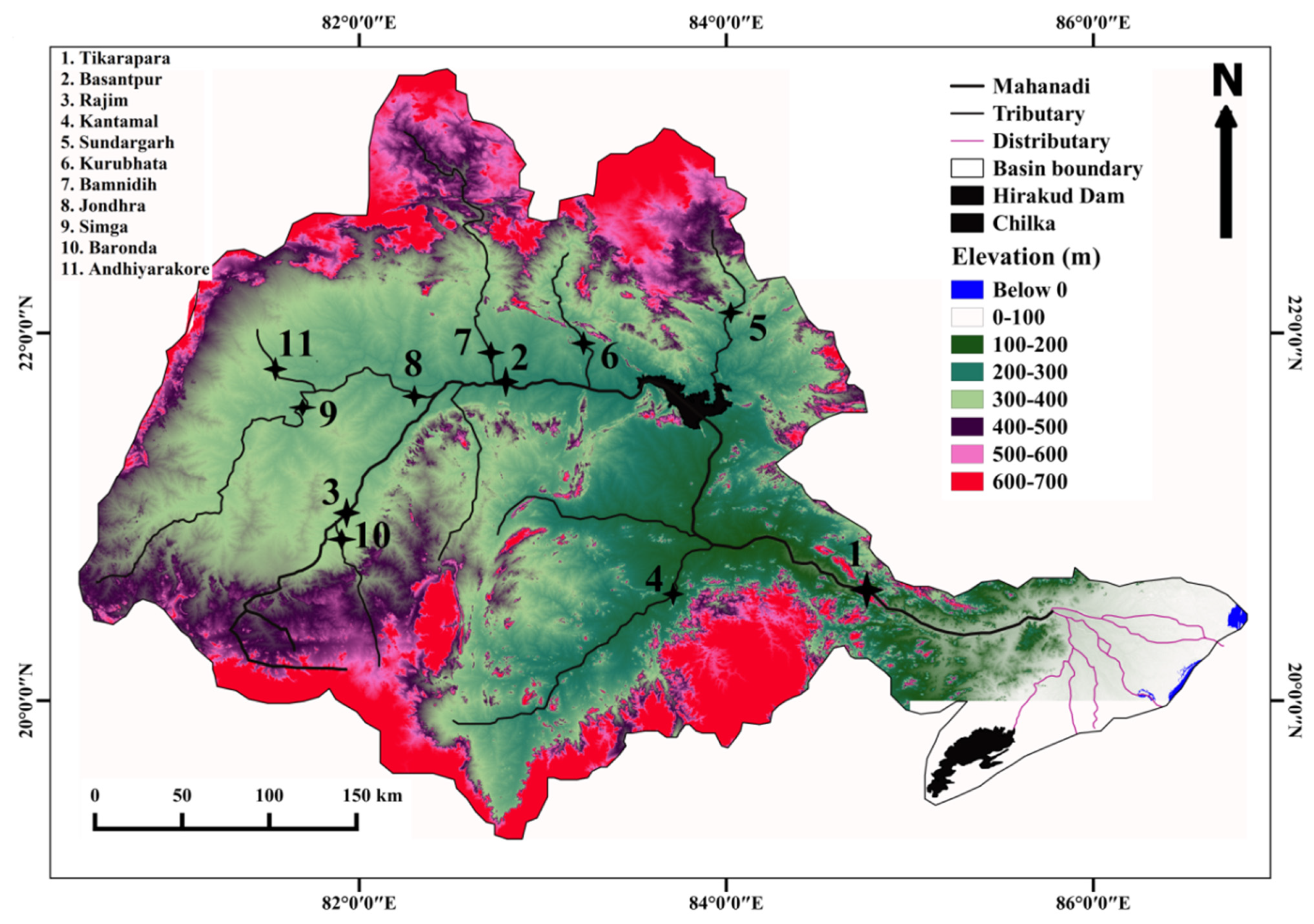
2. Study Area
3. Methodology and Data Used Description
4. Results and Discussion
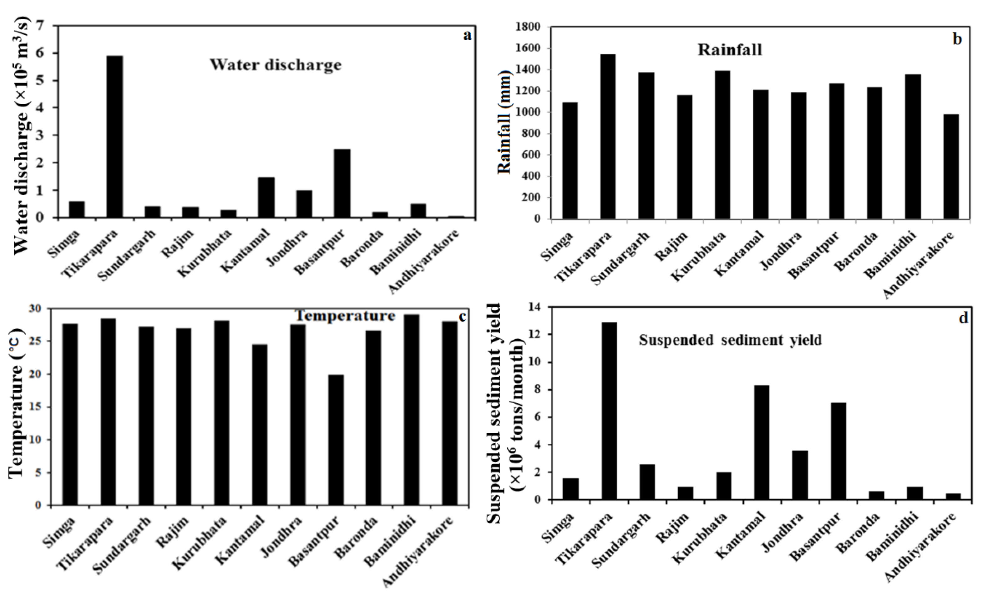
4.1. T-Test of Data and Spatial Variation of Data
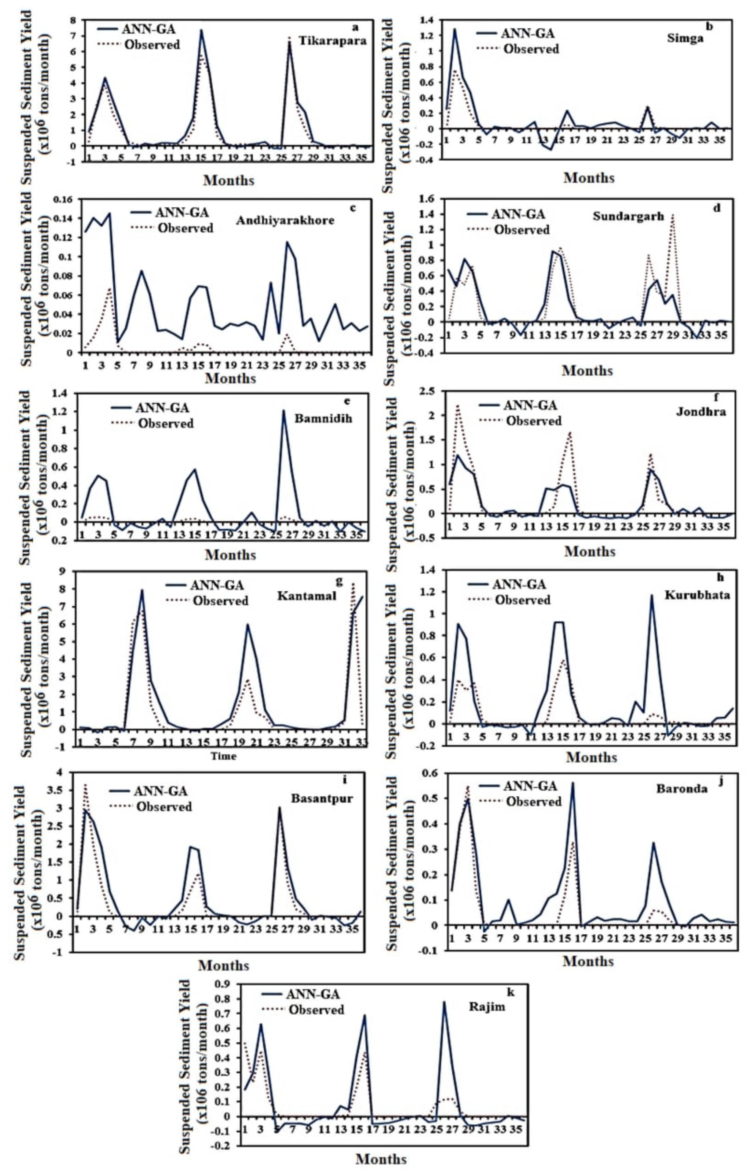
4.2. Hybrid ANN-GA Model for Estimation of SSY
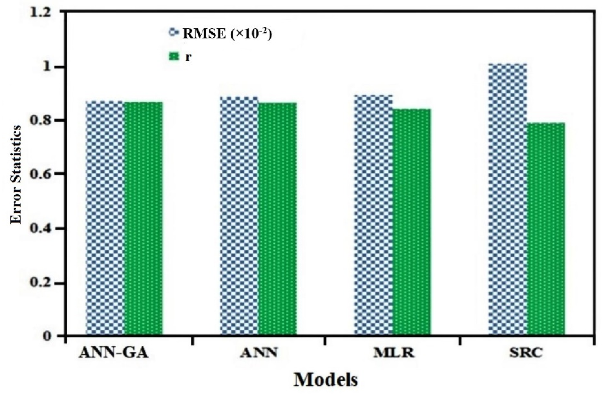
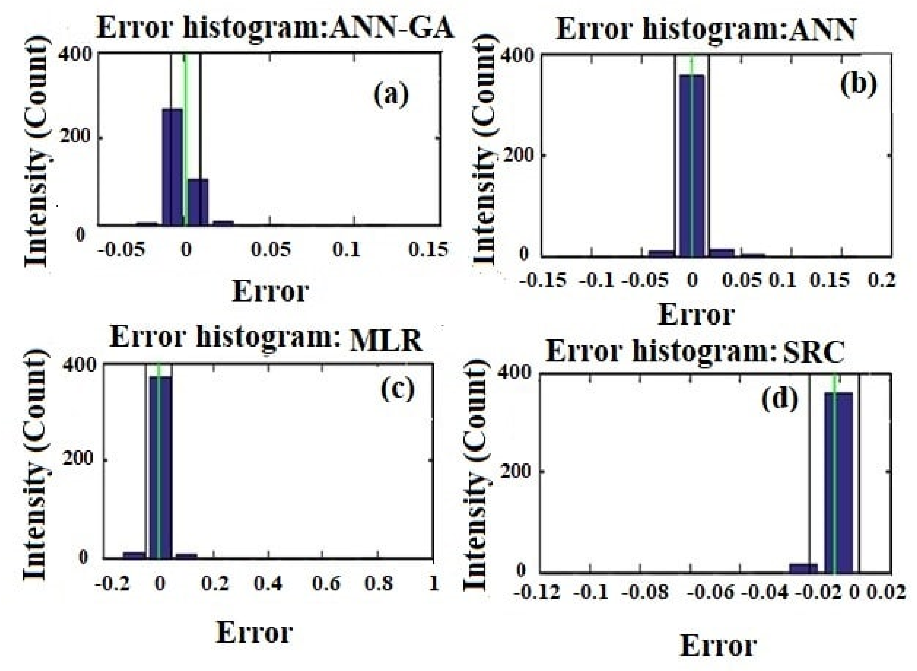
4.3. Comparisons among ANN-GA, SRC, MLR and ANN Models
5. Conclusions
Author Contributions
Funding
Institutional Review Board Statement
Informed Consent Statement
Data Availability Statement
Acknowledgments
Conflicts of Interest
References
- Schumm, S.A. The Fluvial System; John Wiley & Sons: New York, NY, USA, 1977; 338p. [Google Scholar]
- Padmalal, D.; Maya, K. Sand Mining: Environmental Impacts and Selected Case Studies; Sand Mining; Springer: New York, NY, USA; London, UK, 2014. [Google Scholar]
- Newcombe, C.P.; Macdonald, D.D. Effects of Suspended Sediments on Aquatic Ecosystems. N. Am. J. Fish. Manag. 1991, 11, 72–82. [Google Scholar] [CrossRef]
- Mukherjee, S.; Veer, V.; Tyagi, S.K.; Sharma, V. Sedimentation study of Hirakud reservoir through remote sensing techniques. J. Spat. Hydrol. 2007, 7, 122–130. [Google Scholar]
- Walling, D.E. The impact of global change on erosion and sediment transport by rivers. In Current Progress and Future Challenges; United Nations Educational, Scientific and Cultural Organization: Paris, France, 2009. [Google Scholar]
- Fang, N.F.; Shi, Z.H.; Li, L.; Jiang, C. Rainfall, runoff, and suspended sediment delivery relationships in a small agricultural watershed of the Three Gorges area, China. Geomorphology 2011, 135, 158–166. [Google Scholar] [CrossRef]
- Gohil, P.P.; Saini, R.P. Coalesced effect of cavitation and silt erosion in hydro turbines—A review. Renew. Sustain. Energy Rev. 2014, 33, 280–289. [Google Scholar] [CrossRef]
- Kafle, K.R.; Khanal, S.N.; Dahal, R.K. Dynamics of the Koshi River on the Perspective of Morphology and Sedimentation with Emphasis on Post Disaster Impact of the 2008 Koshi Flood. Kathmandu Univ. J. Sci. Eng. Technol. 2015, 11, 71–92. [Google Scholar]
- ZICL. Risk Nexus, Urgent Case for Recovery: What We Can Learn from the August 2014 Karnali River Foods in Nepal; Zurich Insurance Group Ltd.: Zurich, Switzerland, 2014. [Google Scholar]
- Gaurav, K.; Sinha, R.; Panda, P.K. The Indus flood of 2010 in Pakistan: A perspective analysis using remote sensing data. Nat. Hazards 2011, 59, 1815–1826. [Google Scholar] [CrossRef]
- Sinha, R.; Friend, P.F. River systems and their sediment flux, Indo-Gangetic plains, Northern Bihar, India. Sedimentology 1994, 41, 825–845. [Google Scholar] [CrossRef]
- Padhy, M.K.; Saini, R.P. A review on silt erosion in hydro turbines. Renew. Sustain. Energy Rev. 2008, 12, 1974–1987. [Google Scholar] [CrossRef]
- Poudel, L.; Thapa, B.; Shrestha, B.P.; Shrestha, N.K. Sediment impact on turbine material: Case study of Modi River, Nepal. Kathmandu Univ. J. Sci. Eng. Technol. 2012, 8, 88–96. [Google Scholar] [CrossRef]
- Singh, M.; Banerjee, J.; Patel, P.L.; Tiwari, H. Effect of silt erosion on Francis turbine: A case study of Maneri Bhali Stage-II, Uttarakhand, India. ISH J. Hydraul. Eng. 2013, 19, 1–10. [Google Scholar] [CrossRef]
- Loucks, D.P.; Van Beek, E.; Stedinger, J.R.; Dijkman, J.P.; Villars, M.T. Water Resources Systems Planning and Management: An Introduction to Methods, Models and Applications; UNESCO: Paris, France, 2005; 680p. [Google Scholar]
- Kisi, O. Suspended sediment estimation using neuro-fuzzy and neural network approaches. Hydrol. Sci. J. 2005, 50, 683–696. [Google Scholar] [CrossRef]
- Rajaee, T.; Mirbagheri, S.A.; Zounemat-Kermani, M.; Nourani, V. Daily suspended sediment concentration simulation using ANN and neuro-fuzzy models. Sci. Total Environ. 2009, 407, 4916–4927. [Google Scholar] [CrossRef]
- Heng, S.; Suetsugi, T. Using artificial neural network to estimate sediment load in ungauged catchments of the Tonle Sap river basin. Cambodia J. Water Resour. Prot. 2013, 5, 27680. [Google Scholar] [CrossRef]
- Yadav, A.; Prasad, B.B.V.S.V.; Mojjada, R.K.; Kothamasu, K.K.; Joshi, D. Application of Artificial Neural Network and Genetic Algorithm Based Artificial Neural Network Models for River Flow Prediction. Rev. Intell. Artif. 2020, 34, 745–751. [Google Scholar] [CrossRef]
- Wang, X.; Li, Z.; Cai, C.; Shi, Z.; Xu, Q.; Fu, Z.; Guo, Z. Effects of rock fragment cover on hydrological response and soil loss from Regosols in a semi-humid environment in South-West China. Geomorphology 2012, 151, 234–242. [Google Scholar] [CrossRef]
- Biksham, G.; Subramanian, V. Sediment transport of the Godavari River basin and its controlling factors. J. Hydrol. 1988, 101, 275–290. [Google Scholar] [CrossRef]
- Ramesh, R.; Subramanian, V. Temporal, spatial and size variation in the sediment transport in the Krishna River basin, India. J. Hydrol. 1988, 98, 53–65. [Google Scholar] [CrossRef]
- Walling, D.E.; Fang, D. Recent trends in the suspended sediment loads of the world’s rivers. Glob. Planet. Chang. 2003, 39, 111–126. [Google Scholar] [CrossRef]
- Chakrapani, G.J. Factors controlling variations in river sediment loads. Curr. Sci. 2005, 88, 569–575. [Google Scholar]
- Zhu, Y.-M.; Lu, X.X.; Zhou, Y. Sediment flux sensitivity to climate change: A case study in the Longchuanjiang catchment of the upper Yangtze River, China. Glob. Planet. Chang. 2008, 60, 429–442. [Google Scholar] [CrossRef]
- Wood, P.A. Controls of variation in suspended sediment concentration in the River Rother, West Sussex, England. Sedimentology 1977, 24, 437–445. [Google Scholar] [CrossRef]
- Asheghi, R.; Hosseini, S.A.; Sanei, M. Intelligent hybridized modeling approach to predict the bedload sediments in gravel-bed rivers. Modeling Earth Syst. Environ. 2022, 8, 1991–2000. [Google Scholar] [CrossRef]
- Mossa, J. Discharge-Suspended Sediment Relationships in the Mississippi-Atchafalaya Rivers System; Louisiana State University: Baton Rouge, LA, USA, 1990; p. 180. [Google Scholar] [CrossRef]
- Gupta, H.; Chakrapani, G.J. Temporal and spatial variations in water flow and sediment load in Narmada River Basin, India: Natural and man-made factors. Environ. Geol. 2005, 48, 579–589. [Google Scholar] [CrossRef]
- Yadav, A.; Chatterjee, S.; Equeenuddin, S.M. Prediction of Suspended Sediment Yield by Artificial Neural Network and Traditional Mathematical Model in Mahanadi River Basin. India J. Sustain. Water Resour. Manag. 2017, 4, 745–759. [Google Scholar] [CrossRef]
- Bastia, F.; Equeenuddin, S.M. Spatio-temporal variation of water flow and sediment discharge in the Mahanadi River, India. Glob. Planet. Chang. 2016, 144, 51–66. [Google Scholar] [CrossRef]
- Chandramohan, T. Modeling of Suspended Sediment Dynamics in Tropical River Basins. Ph.D. Thesis, Cochin University of Science and Technology, Kochi, India, 2006. [Google Scholar]
- Thodsen, H.; Hasholt, B.; Kjarsgaard, J.H. The influence of climate change on suspended sediment transport in Danish rivers. Hydrol. Process. 2008, 22, 764–774. [Google Scholar] [CrossRef]
- Coulthard, T.J.; Kirkby, M.J.; Macklin, M.G. Modelling geomorphic response to environmental change in an upland catchment. Hydrol. Process. 2000, 14, 2031–2045. [Google Scholar] [CrossRef]
- O’Neal, M.R.; Nearing, M.A.; Vining, R.C.; Southworth, J.; Pfeifer, R.A. Climate change impacts on soil erosion in Midwest United States with changes in crop management. Catena 2005, 61, 165–184. [Google Scholar] [CrossRef]
- Jansson, M.B. Land Erosion by Water in Different Climates. UNGI Report no. 57. Ph.D. Thesis, Department of Physical Geography, University of Uppsala, Uppsala, Sweden, 1982. [Google Scholar]
- Zhu, Y.M.; Lu, X.X.; Zhou, Y. Suspended sediment flux modeling with artificial neural network: An example of the Longchuanjiang River in the Upper Yangtze Catchment, China. Geomorphology 2007, 84, 111–125. [Google Scholar] [CrossRef]
- Fu, S.; Liu, B.; Liu, H.; Xu, L. The effect of slope on interrill erosion at short slopes. Catena 2011, 84, 29–34. [Google Scholar] [CrossRef]
- Jain, S.K. Development of integrated sediment rating curves using ANNs. J. Hydraul. Eng. 2001, 127, 30–37. [Google Scholar] [CrossRef]
- Yadav, A.; Chatterjee, S.; Equeenuddin, S.M. Suspended Sediment Yield Estimation using Genetic Algorithm-based Artificial Intelligence Models in Mahanadi River. Hydrol. Sci. J. 2018, 63, 1162–1182. [Google Scholar] [CrossRef]
- Lenzi, M.A.; Marchi, L. Suspended sediment load during floods in a small stream of the Dolomites (northeastern Italy). Catena 2000, 39, 267–282. [Google Scholar] [CrossRef]
- Khoi, D.N.; Suetsugi, T. The responses of hydrological processes and sediment yield to land-use and climate change in the Be River Catchment, Vietnam. Hydrol. Process. 2014, 28, 640–652. [Google Scholar] [CrossRef]
- Buendia, C.; Bussi, G.; Tuset, J.; Vericat, D.; Sabater, S.; Palau, A.; Batalla, R.J. Effects of afforestation on runoff and sediment load in an upland Mediterranean catchment. Sci. Total Environ. 2016, 540, 144–157. [Google Scholar] [CrossRef]
- Ghaderi, A.; Shahri, A.A.; Larsson, S.A. visualized hybrid intelligent model to delineate Swedish fine-grained soil layers using clay sensitivity. Catena 2022, 214, 106289. [Google Scholar] [CrossRef]
- Hosseini, S.A.; Shahri, A.A.; Asheghi, R. Prediction of bedload transport rate using a block combined network structure. Hydrol. Sci. J. 2022, 67, 117–128. [Google Scholar] [CrossRef]
- Razia, S.; Narasingarao, M.R.; Bojja, P. Development and analysis of support vector machine techniques for early prediction of breast cancer and thyroid. J. Adv. Res. Dyn. Control. Syst. 2017, 9, 869–878. [Google Scholar]
- Patel, A.K.; Chatterjee, S.; Gorai, A.K. Development of an expert system for iron ore classification. Arab. J. Geosci. 2018, 11, 401. [Google Scholar] [CrossRef]
- Patel, A.K.; Chatterjee, S.; Gorai, A.K. Development of a machine vision system using the support vector machine regression (SVR) algorithm for the online prediction of iron ore grades. Earth Sci. Inform. 2019, 12, 197–210. [Google Scholar] [CrossRef]
- Patel, A.K.; Chatterjee, S.; Gorai, A.K. Effect on the performance of a support vector machine-based machine vision system with dry and wet ore sample images in classification and grade prediction. Pattern Recognit. Image Anal. 2019, 29, 309–324. [Google Scholar] [CrossRef]
- Ramaiah, P.; Kumar, S. Dynamic analysis of soil structure interaction (ssi) using anfis model with oba machine learning approach. Int. J. Civ. Eng. Technol. 2018, 9, 496–512. [Google Scholar]
- Dabbakuti, J.R.K.K.; Jacob, A.; Veeravalli, V.R.; Kallakunta, R.K. Implementation of IoT analytics ionospheric forecasting system based on machine learning and ThingSpeak. IET Radar Sonar Navig. 2019, 14, 341–347. [Google Scholar] [CrossRef]
- Karami, H.; Dadras Ajirlou, Y.; Jun, C.; Bateni, S.M.; Band, S.S.; Mosavi, A.; Moslehpour, M.; Chau, K.W. A novel approach for estimation of sediment load in Dam reservoir with hybrid intelligent algorithms. Front. Environ. Sci. 2022, 10, 165. [Google Scholar] [CrossRef]
- Pratuisha, K.; Rajeswarao, D.; Amudhavel, J.; Murthy, J.V.R. A comprehensive study: On artificial-neural network techniques for estimation of coronary-artery disease. Adv. Appl. Math. Sci. 2017, 17, 65–77. [Google Scholar]
- Lakshmi, A.V.; Gopitilak, V.; Parvez, M.M.; Subhani, S.K.; Ghali, V.S. Artificial neural networks based quantitative evaluation of subsurface anomalies in quadratic frequency modulated thermal wave imaging. Infrared Phys. Technol. 2019, 97, 108–115. [Google Scholar] [CrossRef]
- Dabbakuti, J.R.K.K. Application of Singular Spectrum Analysis Using Artificial Neural Networks in TEC Predictions for Ionospheric Space Weather. IEEE J. Sel. Top. Appl. Earth Obs. Remote Sens. 2019, 12, 5101–5107. [Google Scholar] [CrossRef]
- Kisi, O. Multi-layer perceptrons with LevenbergeMarquardt optimization algorithm for suspended sediment concentration prediction and estimation. Hydrol. Sci. J. 2004, 49, 1040. [Google Scholar]
- Bishop, C. Bayesian PCA. In Proceedings of the 11th International Conference on Advances in Neural Information Processing Systems, Denver, CO, USA, 30 November–5 December 1998; pp. 382–388. [Google Scholar]
- Holland, J. Adaptation in Natural and Artificial Systems: An Introductory Analysis with Applications to Biology, Control, and Artificial Intelligence; The University of Michigan Press: Ann Arbor, MI, USA, 1975; p. 232. [Google Scholar]
- Goldberg, D. Genetic Algorithms in Search, Optimization, and Machine Learning, 1st ed.; Addison-Wesley Longman Publishing Co., Inc.: Boston, MA, USA, 1989; p. 372. [Google Scholar]
- Beyer, H.G. Evolutionary algorithms in noisy environments: Theoretical issues and guidelines for practice. Comput. Methods Appl. Mech. Eng. 2000, 186, 239–267. [Google Scholar] [CrossRef]
- Chatterjee, S.; Bandopadhyay, S. Global neural network learning using genetic algorithm for ore grade prediction of iron ore deposit. Min. Resour. Eng. 2007, 12, 258–269. [Google Scholar]
- Chatterjee, S.; Bandopadhyay, S. Goodnews bay platinum resource estimation using least square support vector regression with selection of input space dimension and hyperparameters. Nat. Resour. Res. 2011, 20, 117–129. [Google Scholar] [CrossRef]
- Zhang, D.; Xiao, J.; Zhou, N.; Zheng, M.; Luo, X.; Jiang, H.; Chen, K. A genetic algorithm based support vector machine model for blood-brain barrier penetration prediction. BioMed Res. Int. 2015, 2015, 292683. [Google Scholar] [CrossRef] [PubMed]
- Yadav, A.; Joshi, D.; Kumar, V.; Mohapatra, H.; Iwendi, C.; Gadekallu, T.R. Capability and Robustness of Novel Hybridized Artificial Intelligence Technique for Sediment Yield Modeling in Godavari River, India. Water 2022, 14, 1917. [Google Scholar] [CrossRef]
- Adib, A.; Mahmoodi, A. Prediction of Suspended Sediment Load using ANN GA Conjunction Model with Markov Chain Approach at Flood Conditions. KSCE J. Civ. Eng. 2016, 1, 447–457. [Google Scholar]
- Admuthe, L.; Apte, S.; Admuthe, S. Topology and parameter optimization of ANN using genetic algorithm for application of textiles. In Proceedings of the 5th IEEE International Workshop on Intelligent Data Acquisition and Advanced Computing Systems: Technology and Applications, IDAACS2009, Rende, Italy, 21–23 September 2009; pp. 278–282. [Google Scholar]
- Correa, A.; Gonzalez, A.; Ladino, C. Genetic algorithm optimization for selecting the best architecture of a multi-layer perceptron neural network: A credit scoring case. In SAS Global Forum 2011 Data Mining and Text Analytics; SAS Institute: Cary, NC, USA, 2011. [Google Scholar]
- Anand, K.; Barik, B.K.; Tamilmannan, K.; Sathiya, P. Artificial neural network modeling studies to predict the friction welding process parameters of Incoloy 800H joints. Eng. Sci. Technol. Int. J. 2015, 18, 394–407. [Google Scholar] [CrossRef]
- Chau, K.W.; Wu, C.; Li, Y.S. Comparison of several flood forecasting models in Yangtze River. J. Hydrol. Eng. 2005, 10, 485–491. [Google Scholar] [CrossRef]
- Chatterjee, S.; Bandopadhyay, S. Reliability estimation using a genetic algorithm-based artificial neural network: An application to a laud-haul-dump machine. Expert Syst. Appl. 2012, 39, 10943–10951. [Google Scholar] [CrossRef]
- Parasuraman, K.; Elshorbagy, A. Cluster-Based Hydrologic Prediction Using Genetic Algorithm-Trained Neural Networks. J. Hydrol. Eng. 2007, 12, 52–62. [Google Scholar] [CrossRef]
- Sedki, A.D.; Ouazar, D.; Mazoudi, E. Evolving Neural Network Using Real Coded Genetic Algorithm for Daily Rainfall-Runoff Forecasting. Expert Syst. Appl. 2009, 36, 4523–4527. [Google Scholar] [CrossRef]
- Asadi, S.; Shahrabi, J.; Abbaszadeh, P.; Tabanmehr, S. A New Hybrid Artificial Neural Networks for Rainfall-Runoff Process Modeling. Neurocomputing 2013, 121, 470–480. [Google Scholar] [CrossRef]
- Sirdari, Z.Z.; Ghani, A.A.; Sirdari, N.Z. Bedload transport predictions based on field measurement data by combination of artificial neural network and genetic programming. Pollution 2014, 1, 85–94. [Google Scholar]
- Adib, A.; Jahanbakhshan, H. Stochastic approach to determination of suspended sediment concentration in tidal rivers by artificial neural network and genetic algorithm. Can. J. Civ. Eng. 2013, 40, 299–312. [Google Scholar] [CrossRef]
- Pektas, A.O.; Cigizoglu, H.K. Long-range forecasting of suspended sediment. Hydrol. Sci. J. 2017, 62, 2415–2425. [Google Scholar] [CrossRef]
- Yadav, A.; Chatterjee, S.; Equeenuddin, S.M. Suspended sediment yield modeling in Mahanadi River, India by multi-objective optimization hybridizing artificial intelligence algorithms. Int. J. Sediment Res. 2020, 36, 76–91. [Google Scholar] [CrossRef]
- Agrawal, S.; Sarkar, S.; Srivastava, G.; Maddikunta, P.K.; Gadekallu, T.R. Genetically optimized prediction of remaining useful life. Sustain. Comput. Inform. Syst. 2021, 31, 100565. [Google Scholar] [CrossRef]
- Agrawal, S.; Sarkar, S.; Alazab, M.; Maddikunta, P.K.; Gadekallu, T.R.; Pham, Q.V. Genetic CFL: Hyperparameter optimization in clustered federated learning. Comput. Intell. Neurosci. 2021, 2021, 7156420. [Google Scholar] [CrossRef]
- Ch, A.; Ch, R.; Gadamsetty, S.; Iwendi, C.; Gadekallu, T.R.; Dhaou, I.B. ECDSA-Based Water Bodies Prediction from Satellite Images with UNet. Water 2022, 14, 2234. [Google Scholar] [CrossRef]
- India-WRIS. Water Resources Information System of India. Available online: http://india-wris.nrsc.gov.in/wrpinfo/index.php?title=Mahanadi (accessed on 8 August 2016).
- Samantaray, S.; Ghose, D.K. Evaluation of suspended sediment concentration using descent neural networks. Procedia Comput. Sci. 2018, 132, 1824–1831. [Google Scholar] [CrossRef]
- Ghosh, U.; Luthy, R.G.; Cornelissen, G.; Werner, D.; Menzie, C.A. In-situ sorbent amendments: A new direction in contaminated sediment management. Environ. Sci. Technol. 2011, 45, 1163–1168. [Google Scholar] [CrossRef]
- Kant, A.; Suman, P.K.; Giri, B.K.; Tiwari, M.K.; Chatterjee, C.; Nayak, P.C.; Kumar, S. Comparison of multi-objective evolutionary neural network, adaptive neuro-inference system and bootstrap-based neural network for flood forecasting. Neural Comput. Appl. 2013, 23, 231–246. [Google Scholar] [CrossRef]
- Pramanik, N.; Panda, R.K. Application of neural network and adaptive neuro-fuzzy inference systems for river flow prediction. Hydrol. Sci. J. 2009, 54, 247–260. [Google Scholar] [CrossRef]
- Central Water Commission (CWC). Integrated Hydrological Data Book. Hydrological Data Directorate; Information Systems Organization, Water Planning and Projects Wing: New Delhi, India, 2012. [Google Scholar]
- Water Year Book; Central Water Commission, Government of India: Delhi, India, 1997.
- Panigrahy, B.K.; Raymahashay, B.C. River water quality in weathered limestone: A case study in upper Mahanadi basin, India. J. Earth Syst. Sci. 2005, 114, 533–543. [Google Scholar] [CrossRef]
- Chakrapani, G.J.; Subramanian, V. Rates of erosion and sedimentation in the Mahanadi River basin, India. J. Hydrol. 1993, 149, 39–48. [Google Scholar] [CrossRef]
- Rojas, R. Neural Network: A Systematic Introduction; Springer: Berlin, Germany, 1996; pp. 151–184. [Google Scholar]
- Boukhrissa, Z.A.; Khanchoul, K.; Le Bissonnais, Y.; Tourki, M. Prediction of sediment load by sediment rating curve and neural network (ANN) in El Kebir catchment. Alger. J. Earth Syst. Sci. 2013, 122, 1303–1312. [Google Scholar] [CrossRef]
- Kisi, O.; Shree, J. River suspended sediment estimation by climatic variables implication: Comparative study among soft computing techniques. Comput. Geosci. 2012, 43, 73–82. [Google Scholar] [CrossRef]
- Davis, L. Handbook of Genetic Algorithms; Van Nostrand Reinhold: New York, NY, USA, 1991. [Google Scholar]
- Zanaganeh, M.; Mousavi, S.J.; Sahidi, A.F.E. A hybrid genetic algorithm-adaptive neural network based fuzzy inference system in prediction of wave parameter. Eng. Appl. Artif. Intell. 2009, 22, 1194–1202. [Google Scholar] [CrossRef]
- DeJong, K. An Analysis of the Behavior of a Class of Genetic Adaptive Systems. Ph.D. Thesis, University of Michigan, Ann Arbor, MI, USA, 1975. [Google Scholar]
- Tahmasebi, P.; Hezarkhani, A. Application of Optimized Neural Network by Genetic Algorithm; Stanford University: Stanford, CA, USA, 2009; Volume 2, pp. 15–23. [Google Scholar]
- Gray, J.R.; Landers, M.N. Measuring suspended sediment. In Comprehensive Water Quality and Purification; Ahuja, S., Ed.; Elsevier: Amsterdam, The Netherlands, 2014; Volume 1, pp. 157–204. [Google Scholar]
- Tassone, B.; Lapointe, F. Suspended-Sediment Sampling, Hydrometric Technician Career Development Program; The Water Survey of Cannada: Ottawa, ON, Canada, 1999; Available online: http://publications.gc.ca/collections/collection_2014/ec/En56-247-1999-eng.pdf (accessed on 5 January 2022).
- Altun, H.; Bilgil, A.; Fidan, B.C. Treatment of multidimensional data to enhance neural network estimators in regression problems. Expert Syst. Appl. 2007, 32, 599–605. [Google Scholar] [CrossRef]
- Panda, D.K.; Kumar, A.; Mohanty, S. Recent trends in sediment load of the tropical (Peninsular) river basins of India. Glob. Planet. Chang. 2011, 75, 108–118. [Google Scholar] [CrossRef]
- Jin, L.; Whitehead, P.G.; Rodda, H.; Macadam, I.; Sarkar, S. Simulating climate change and socio-economic change impacts on flows and water quality in the Mahanadi River system, India. Sci. Total Environ. 2018, 637, 907–917. [Google Scholar] [CrossRef]
- Loo, Y.Y.; Billa, L.; Singh, A. Effect of climate change on seasonal monsoon in Asia and its impact on the variability of monsoon rainfall in Southeast Asia. Geosci. Front. 2015, 6, 817–823. [Google Scholar] [CrossRef]
- Ahmed, M.M.; Hasan, M.K.; Shafiq, M.; Qays, M.O.; Gadekallu, T.R.; Nebhen, J.; Islam, S. A peer-to-peer blockchain based interconnected power system. Energy Rep. 2021, 7, 7890–7905. [Google Scholar] [CrossRef]
- Hasan, M.K.; Akhtaruzzaman, M.; Kabir, S.R.; Gadekallu, T.R.; Islam, S.; Magalingam, P.; Hassan, R.; Alazab, M.; Alazab, M.A. Evolution of industry and blockchain era: Monitoring price hike and corruption using BIoT for smart government and industry 4.0. IEEE Trans. Ind. Inform. 2022. [Google Scholar] [CrossRef]
- Abdullah, A.; Ting, W.E. Orientation and Scale Based Weights Initialization Scheme for Deep Convolutional Neural Networks. Asia-Pac. J. Inf. Technol. Multimed. 2020, 9, 103–112. [Google Scholar] [CrossRef]
- Zavvar, M.O.; Garavand, S.H.; Nehi, M.R.; Yanpi, A.M.; Rezaei, M.E.; Zavvar, M.H. Measuring reliability of aspect-oriented software using a combination of artificial neural network and imperialist competitive algorithm. Asia-Pac. J. Inf. Technol. Multimed. 2017, 5, 75–85. [Google Scholar] [CrossRef]
- Tan, T.G.; Teo, J.; Chin, K.; Alfred, R. A coevolutionary multiobjective evolutionary algorithm for game artificial intelligence. Asia Pac. J. Inf. Technol. Multimed. 2013, 2, 53–61. [Google Scholar] [CrossRef]
- Chakrapani, G.J.; Subramanian, V. Factors controlling sediment discharge in the Mahanadi River Basin. India. J. Hydrol. 1990, 117, 169–185. [Google Scholar] [CrossRef]
- Dai, Z.; Liu, J.T.; Wei, W.; Chen, J. Detection of the Three Gorges Dam influence on the Changjiang (Yangtze River) submerged delta. Sci. Rep. 2014, 4, 6600. [Google Scholar] [CrossRef]
- Yue, Z.; Xixi, L.; Ying, H.; Yunmei, Z. Anthropogenic impact on the sediment flux in the dry-hot valleys of Southwest China-an example of the Longchaun River. J. Mt. Sci. 2004, 1, 239–249. [Google Scholar] [CrossRef]
- Lu, X.X. Spatial variability and temporal changed of water discharge and sediment flux in the lower Jinsha tributary: Impact of environmental changes. River Res. Appl. 2005, 21, 229–243. [Google Scholar] [CrossRef]
- Sandy, R. Statistics for Business and Economics; McGraw-Hill Publishing: New York, NY, USA, 1990; p. 1117. [Google Scholar]
- Yadav, A.; Satyannarayana, P. Multi-objective genetic algorithm optimization of artificial neural network for estimating suspended sediment yield in Mahanadi River basin, India. Int. J. River Basin Manag. 2020, 18, 207–215. [Google Scholar] [CrossRef]
- Gärdenfors, P.; Sahlin, N.E. Unreliable probabilities, risk taking, and decision making. Synthese 1982, 53, 361–386. [Google Scholar] [CrossRef]
- Barford, N.C. Experimental Measurements: Precision, Error, and Truth; Wiley–Blackwell: New York, NY, USA, 1985. [Google Scholar]
- Kennedy, M.C.; O’Hagan, A. Bayesian calibration of computer models. J. R. Stat. Soc. Ser. B (Stat. Methodol.) 2001, 63, 425–464. [Google Scholar] [CrossRef]
- Yan, H.; Ma, T. A group decision-making approach to uncertain quality function deployment based on fuzzy preference relation and fuzzy majority. Eur. J. Oper. Res. 2015, 241, 815–829. [Google Scholar] [CrossRef]
- Zhang, J.; Yin, J.; Wang, R. Basic framework and main methods of uncertainty quantification. Mater. Probl. Eng. 2020, 2020, 6068203. [Google Scholar] [CrossRef]
- Jiang, C.; Zheng, J.; Han, X. Probability–interval hybrid uncertainty analysis for structures with both aleatory and epistemic uncertainties: A review. Struct. Multidiscip. Optim. 2018, 57, 2485–2502. [Google Scholar] [CrossRef]
- Cacuci, D.G.; Ionescu-Bujor, M. A comparative review of sensitivity and uncertainty analysis of large–scale systems–II: Statistical methods. Nucl. Sci. Eng. 2004, 147, 204–217. [Google Scholar] [CrossRef]
- Ahmed, Z.E.; Hasan, M.K.; Saeed, R.A.; Hassan, R.; Islam, S.; Mokhtar, R.A.; Khan, S.; Akhtaruzzaman, M. Optimizing energy consumption for cloud internet of things. Front. Phys. 2020, 8, 358. [Google Scholar] [CrossRef]
- Latiffi, M.I.A.; Yaakub, M.R. Sentiment analysis: An enhancement of ontological-based using hybrid machine learning techniques. Asia-Pac. J. Inf. Technol. Multimed. 2018, 7, 61–69. [Google Scholar] [CrossRef]


| Data Set | t-Test | Water-Discharge | Rainfall | Temperature | Suspended Sediment Yield |
|---|---|---|---|---|---|
| Training and testing | p | 0.9013 | 0.5932 | 0.2339 | 0.2392 |
| t | 0.1230 | 0.5328 | 1.1632 | −131.2 | |
| Training and validation | p | 0.9630 | 0.8957 | 0.2863 | 0.0855 |
| t | −0.0352 | −0.1311 | 1.0663 | 1.7205 | |
| Validation and testing | p | 0.8838 | 0.5935 | 0.9259 | 0.5603 |
| t | 0.1339 | 0.5326 | 0.0930 | −0.5827 |
| Stations | Q-SSY(r1) | RF-SSY(r2) | T-SSY(r3) |
|---|---|---|---|
| Tikarapara | 0.9323 | 0.5787 | 0.1499 |
| Simga | 0.8528 | 0.5736 | −0.0865 |
| Andhiyarakhore | 0.8218 | 0.5847 | 0.1866 |
| Sundargarh | 0.8913 | 0.7917 | 0.1459 |
| Bamnidih | 0.7924 | 0.4963 | 0.1082 |
| Jondhara | 0.8873 | 0.5711 | 0.1437 |
| Kantamal | 0.8492 | 0.6643 | 0.1038 |
| Kurubhata | 0.9031 | 0.7866 | 0.1734 |
| Basantpur | 0.8935 | 0.6941 | 0.1516 |
| Baronda | 0.8224 | 0.6467 | 0.0677 |
| Rajim | 0.8413 | 0.6377 | 0.0624 |
| ANN-GA | RMSE | MSE | MAE | Variance | r | Coefficient of Eficiency |
|---|---|---|---|---|---|---|
| Training | 0.0048 | 2.390 × 10−05 | 0.002 | 2.390 × 10−05 | 0.972 | 0.956 |
| Validation | 0.014 | 2.000 × 10−04 | 0.004 | 1.000 × 10−03 | 0.752 | −0.081 |
| Testing | 0.009 | 7.660 × 10−05 | 0.003 | 7.550 × 10−05 | 0.871 | 0.667 |
| Tikarapara | 0.007 | 5.260 × 10−05 | 0.006 | 5.530 × 10−05 | 0.980 | 0.936 |
| Simga | 0.008 | 5.890 × 10−05 | 0.001 | 5.820 × 10−06 | 0.921 | 0.251 |
| Andhiyakore | 0.001 | 8.550 × 10−07 | 0.001 | 2.830 × 10−07 | 0.688 | −18.810 |
| Sundargarh | 0.004 | 1.710 × 10−05 | 0.002 | 1.750 × 10−05 | 0.721 | 0.558 |
| Bamnidih | 0.005 | 2.090 × 10−05 | 0.003 | 1.900 × 10−05 | 0.906 | −259 |
| Jondhara | 0.005 | 2.950 × 10−05 | 0.003 | 2.920 × 10−05 | 0.830 | 0.627 |
| Kantamal | 0.032 | 1.000 × 10−03 | 0.013 | 7.000 × 10−04 | 0.778 | 0.259 |
| Kurubhata | 0.004 | 1.900 × 10−05 | 0.003 | 1.630 × 10−05 | 0.732 | −2.201 |
| Basantpur | 0.007 | 5.120 × 10−05 | 0.005 | 3.970 × 10−05 | 0.917 | 0.772 |
| Baronda | 0.001 | 1.770 × 10−06 | 0.001 | 1.220 × 10−06 | 0.890 | 0.555 |
| Rajim | 0.003 | 6.330 × 10−06 | 0.002 | 6.550 × 10−06 | 0.752 | −0.356 |
| Gauge Station | Time Index of Peaks | Q (m3/s) | RF (mm) | Sediment Yield (Tons/Month) | T (°C) |
|---|---|---|---|---|---|
| Sundargarh | 2 | 7756 | 351 | 582,190 | 27 |
| 4 | 11,857 | 242 | 732,762 | 29.5 | |
| 15 | 11,239 | 488 | 970,420 | 27.5 | |
| 26 | 8164 | 591 | 863,698 | 28.5 | |
| 29 | 6488 | 169 | 1,386,340 | 26 | |
| Kurubhata | 2 | 4551 | 406 | 403,901 | 29.5 |
| 4 | 6463 | 207 | 371,259 | 31 | |
| 15 | 9845 | 529 | 578,737 | 29 | |
| 26 | 3130 | 566 | 90,388 | 26.5 | |
| Jondhra | 2 | 42,770 | 404 | 2,225,625 | 30.5 |
| 16 | 19,207 | 152 | 1,660,837 | 30.75 | |
| 26 | 25,906 | 508 | 1,226,185 | 30.75 | |
| Baronda | 3 | 12,363 | 245 | 550,873 | 29.25 |
| 15 | 13,228 | 267 | 330,656 | 28.75 | |
| 26 | 2668 | 592 | 57,911 | 29.25 | |
| Baminidhi | 3 | 6138 | 428 | 53,056 | 29.5 |
| 15 | 5877 | 441 | 40,044 | 29 | |
| 26 | 3256 | 636 | 58,940 | 34 | |
| Andhiyarakhore | 4 | 1244 | 233 | 67,731 | 28.5 |
| 15 | 325 | 139 | 8615 | 28 | |
| 26 | 220 | 334 | 19,228 | 31.5 |
Publisher’s Note: MDPI stays neutral with regard to jurisdictional claims in published maps and institutional affiliations. |
© 2022 by the authors. Licensee MDPI, Basel, Switzerland. This article is an open access article distributed under the terms and conditions of the Creative Commons Attribution (CC BY) license (https://creativecommons.org/licenses/by/4.0/).
Share and Cite
Yadav, A.; Hasan, M.K.; Joshi, D.; Kumar, V.; Aman, A.H.M.; Alhumyani, H.; Alzaidi, M.S.; Mishra, H. Optimized Scenario for Estimating Suspended Sediment Yield Using an Artificial Neural Network Coupled with a Genetic Algorithm. Water 2022, 14, 2815. https://doi.org/10.3390/w14182815
Yadav A, Hasan MK, Joshi D, Kumar V, Aman AHM, Alhumyani H, Alzaidi MS, Mishra H. Optimized Scenario for Estimating Suspended Sediment Yield Using an Artificial Neural Network Coupled with a Genetic Algorithm. Water. 2022; 14(18):2815. https://doi.org/10.3390/w14182815
Chicago/Turabian StyleYadav, Arvind, Mohammad Kamrul Hasan, Devendra Joshi, Vinod Kumar, Azana Hafizah Mohd Aman, Hesham Alhumyani, Mohammed S. Alzaidi, and Haripriya Mishra. 2022. "Optimized Scenario for Estimating Suspended Sediment Yield Using an Artificial Neural Network Coupled with a Genetic Algorithm" Water 14, no. 18: 2815. https://doi.org/10.3390/w14182815