
Salinity and Temperature Variations near the Freshwater-Saltwater Interface in Coastal Aquifers Induced by Ocean Tides and Changes in Recharge
 , ,
, ,
Abstract
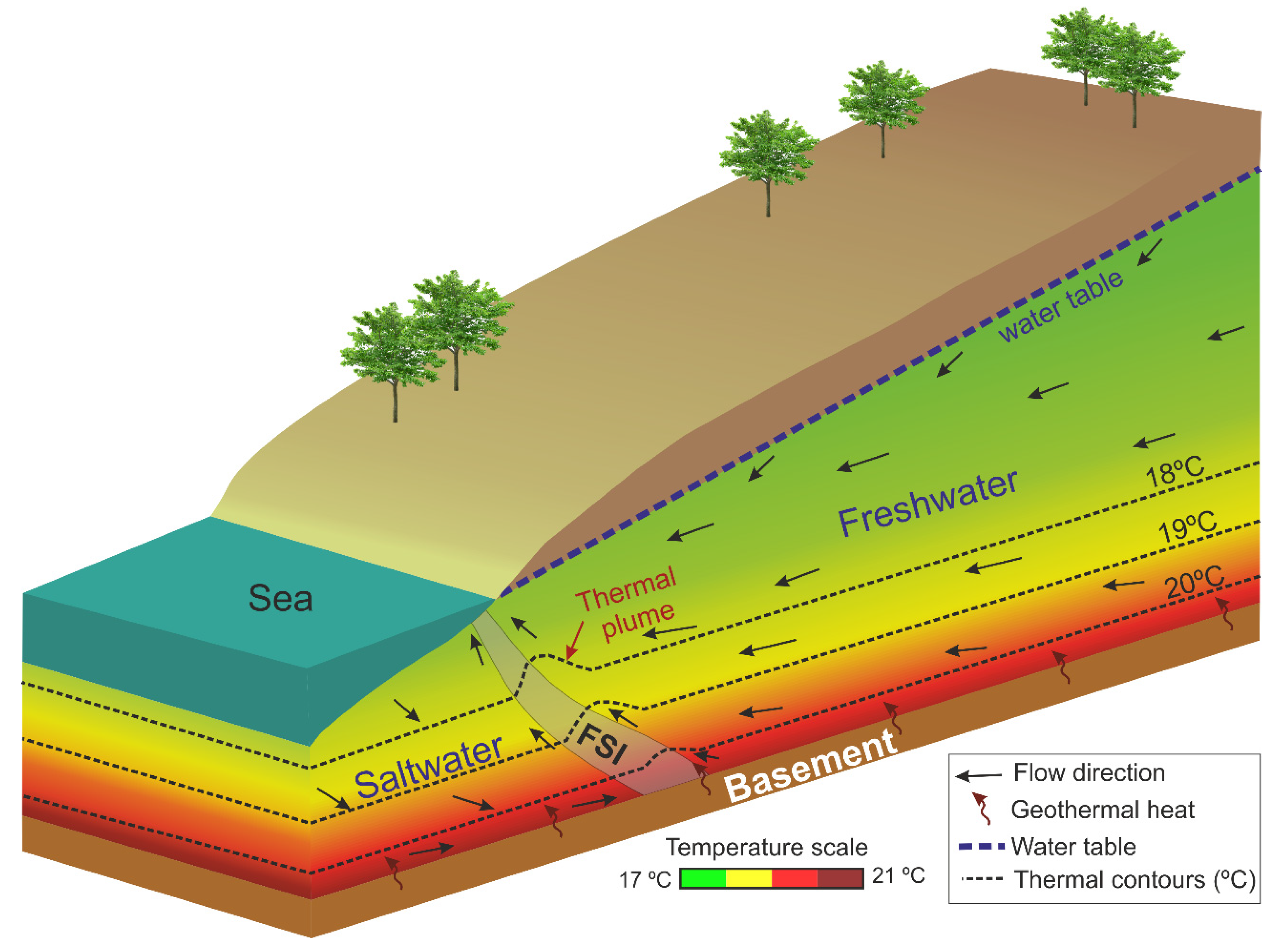
:1. Introduction
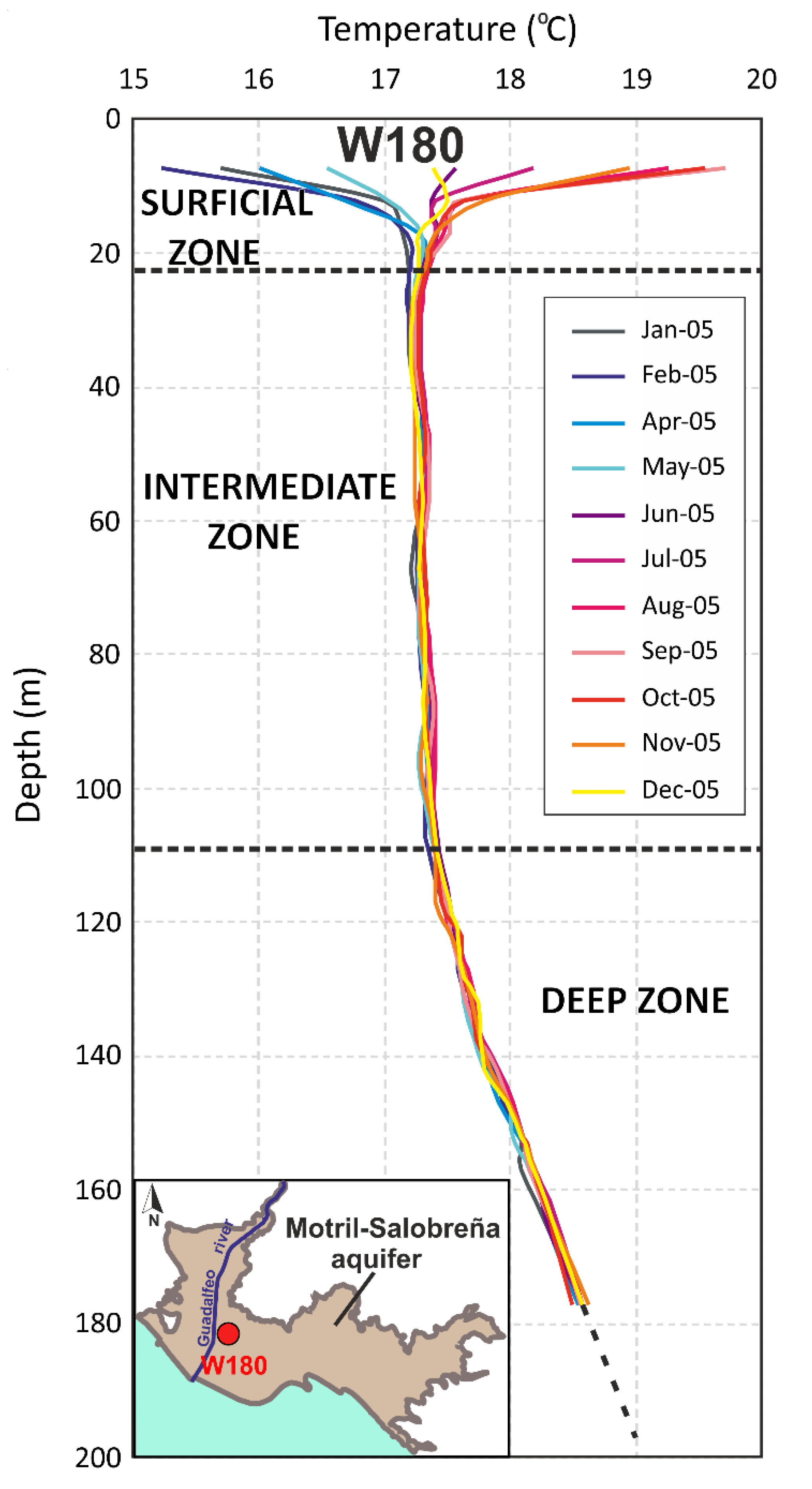
2. Study Area and Hydrogeological Setting

3. Methodology
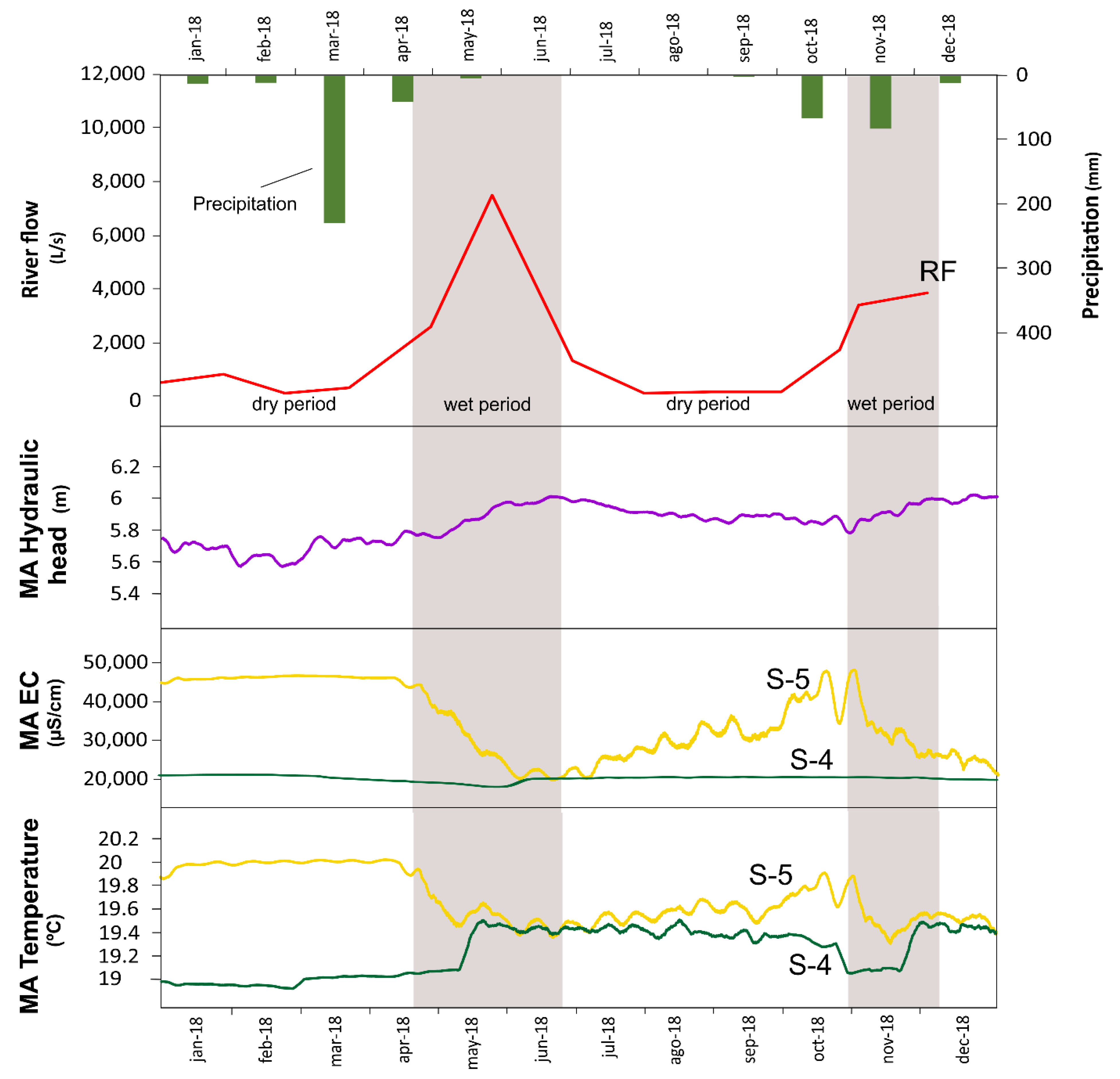
3.1. Field Monitoring
3.2. Time Series Analysis
3.3. Numerical Modeling
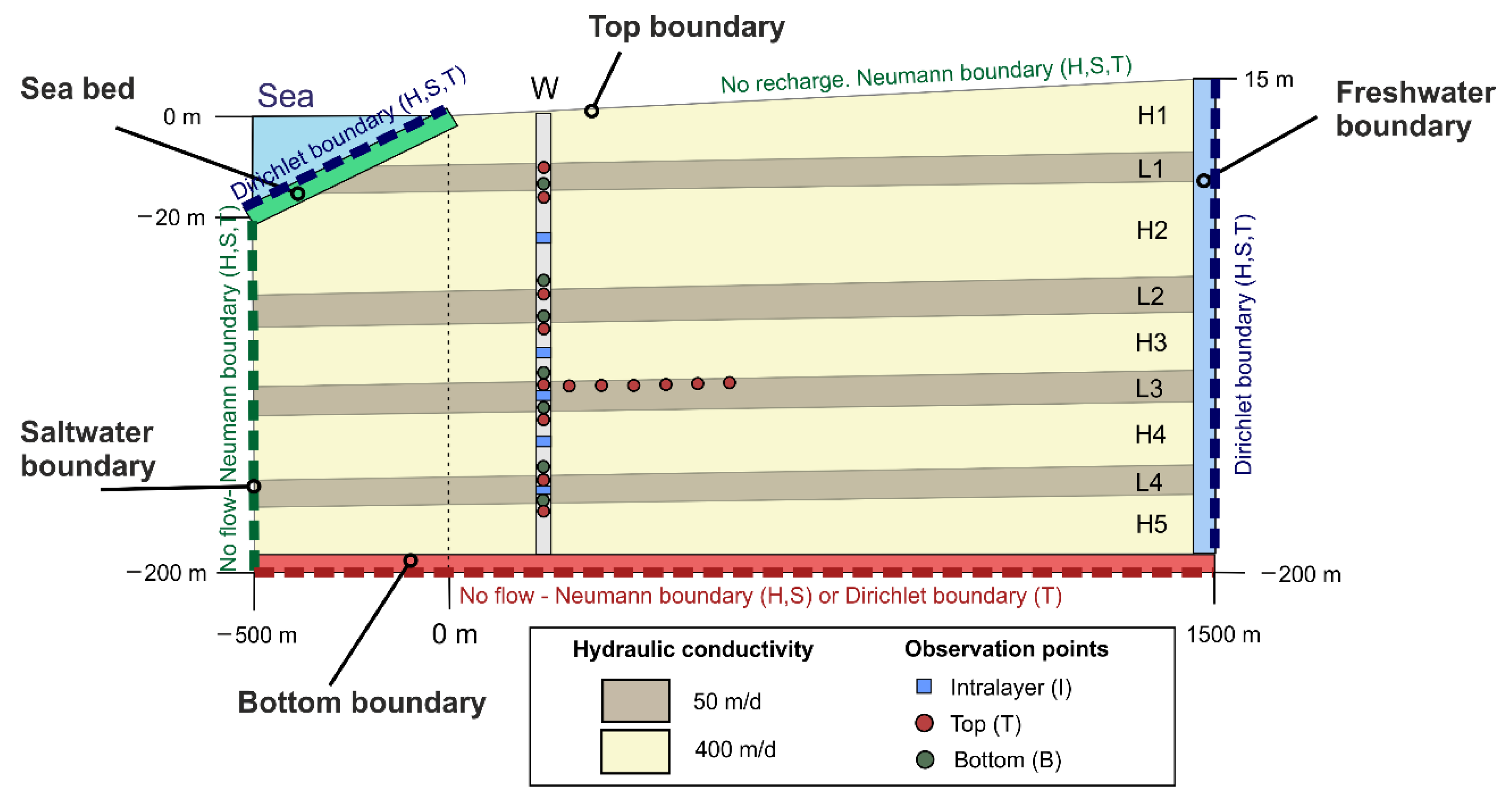
3.3.1. Models
- -
- Model A (Homogeneous model): the hydraulic conductivity was homogeneous (100 m/d).
- -
- Model B (Heterogeneous layered model): nine layers with different hydraulic conductivity (50 and 400 m/d) were included to modify model A. The thickness of the layers was 15 m for the layers with lower hydraulic conductivity (L1, L2, L3 and L4) and 20–45 m for the layers with higher hydraulic conductivity (H1, H2, H3 and H4) (Figure 4). The alternation of layers with the two values of hydraulic conductivity represented the vertical heterogeneity often found in alluvial coastal aquifers.
- -
- Model C (Changes in recharge conditions): the model parameters were the same as those of model B, but the recharge effect was simulated, modifying the boundary conditions to reproduce a gradually increasing hydraulic gradient, justified by fluctuations of the water table in the upper sector of the aquifer (up to 5 m from summer to winter), and by the lack of recharge of the river near the coastline [45].
3.3.2. Boundary Conditions

| Model | Parameter | Freshwater | Sea Bed | Saltwater | Top | Bottom |
|---|---|---|---|---|---|---|
| Model A | H | Dirichlet 8 m | Dirichlet | Neumann No flow | Neumann No flow | Neumann No flow |
| S | Dirichlet 350 mg/L | Dirichlet 35,000 mg/L | Neumann No flow | Neumann No flow | Neuman No flow | |
| T | Dirichlet 17 °C | Dirichlet 13 °C | Neumann No flow | Neumann No flow | Dirichlet 24 °C | |
| Model B | H | Dirichlet 8 m | Dirichlet | Neumann No flow | Neumann No flow | Neumann No flow |
| S | Dirichlet 350 mg/L | Dirichlet 35,000 mg/L | Neumann No flow | Neumann No flow | Neuman No flow | |
| T | Dirichlet 17 °C | Dirichlet 13 °C | Neumann No flow | Neumann No flow | Dirichlet 24 °C | |
| Model C | H | Dirichlet 8 to 13 m | Dirichlet | Neumann No flow | Neumann No flow | Neumann No flow |
| S | Dirichlet 350 mg/L | Dirichlet 35,000 mg/L | Neumann No flow | Neumann No flow | Neuman No flow | |
| T | Dirichlet 17 °C | Dirichlet 13 °C | Neumann No flow | Neumann No flow | Dirichlet 24 °C |
3.3.3. Parameters and Time Discretization
4. Results
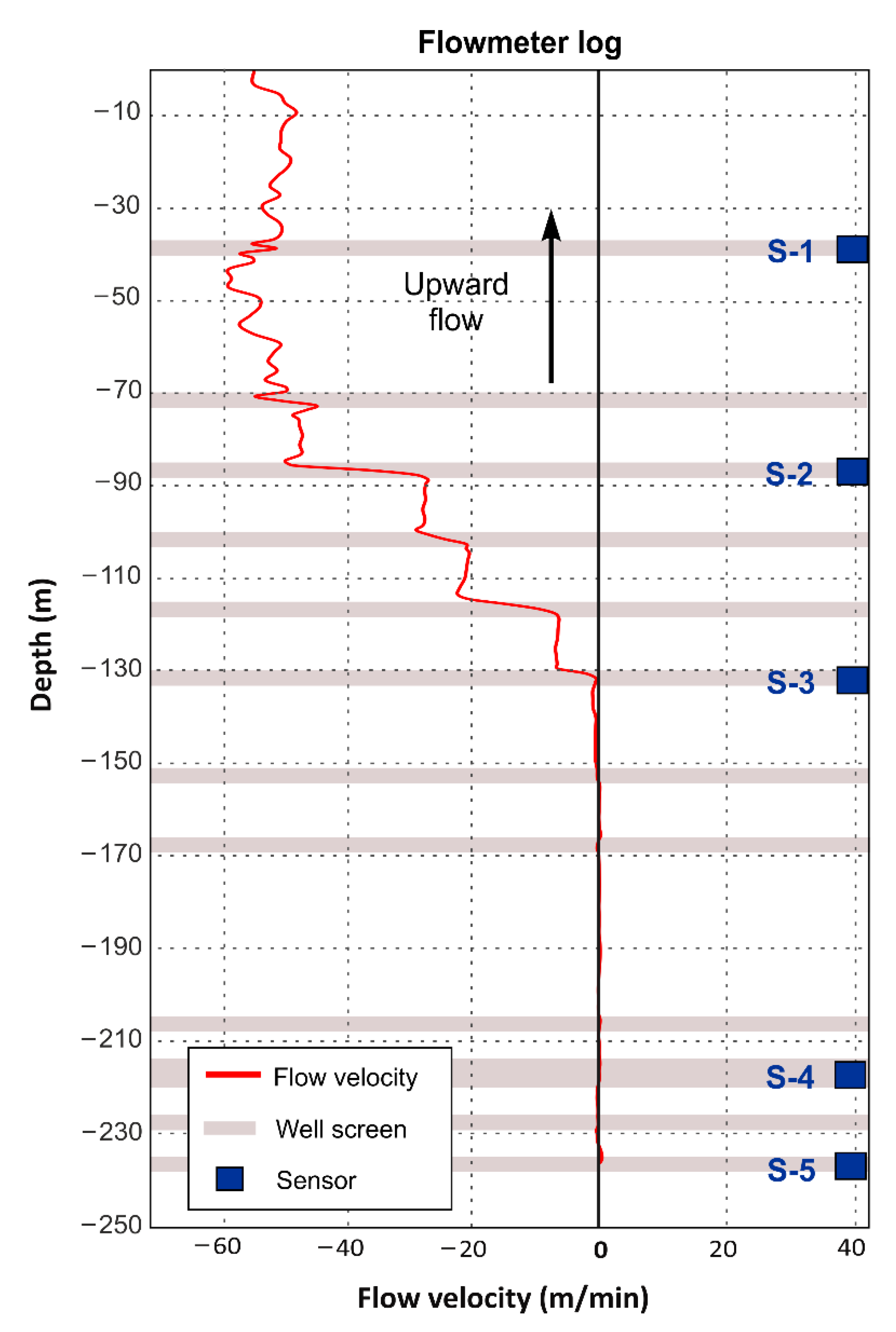
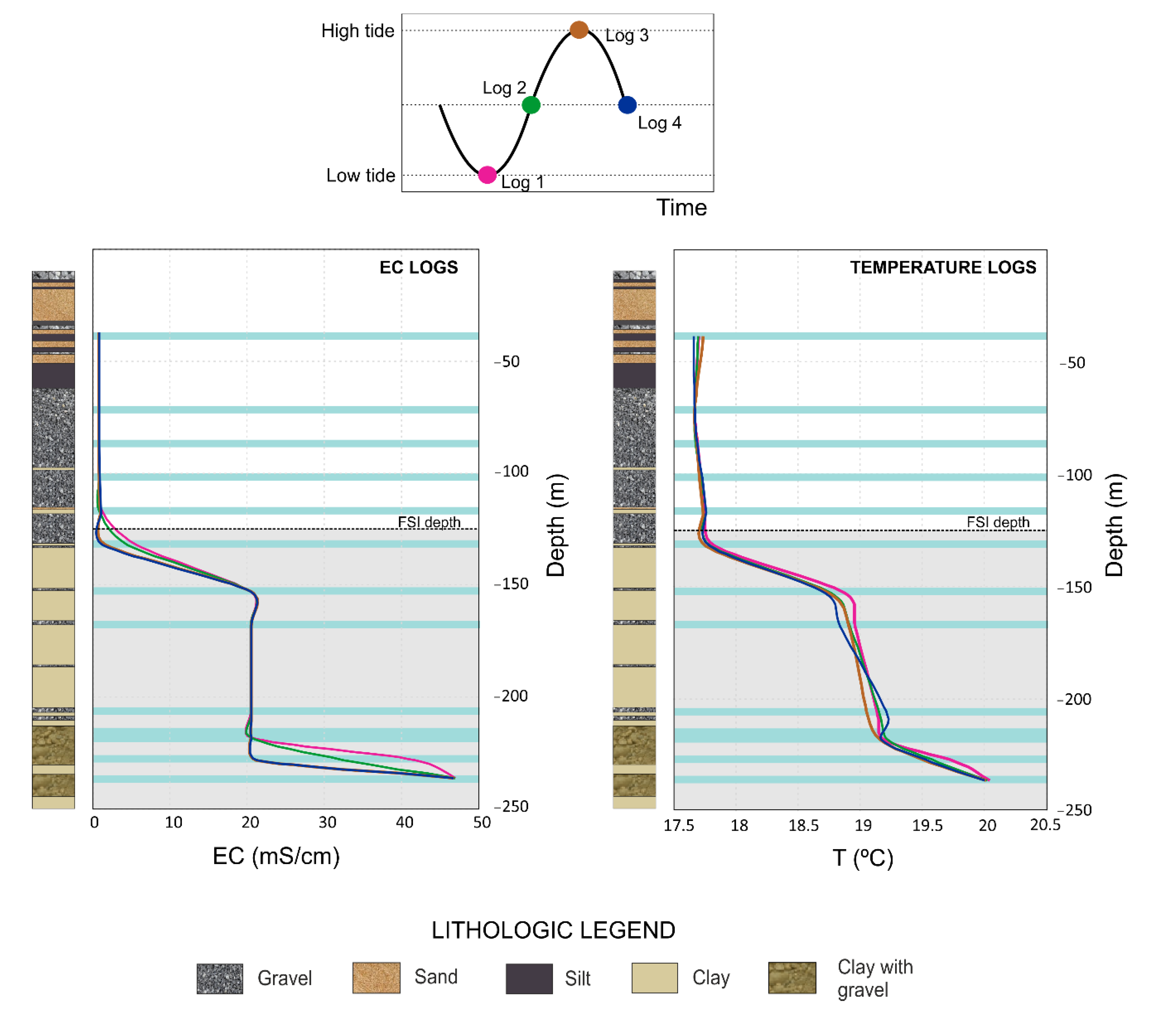
4.1. Vertical Flow in the Borehole
4.2. Water Table Variation Effect on Temperature Oscillation in the FSI
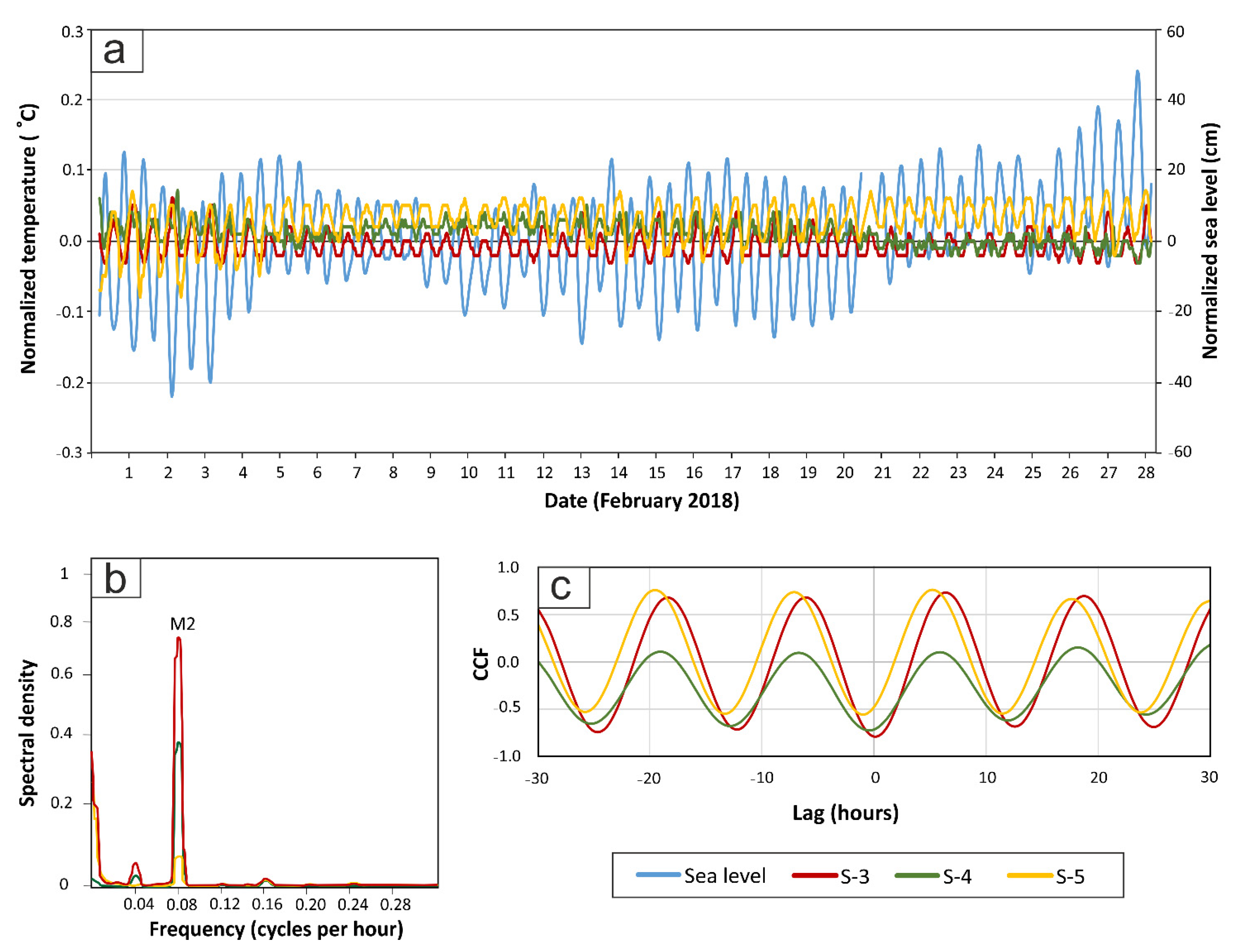
4.3. Sea Tides Effect on Temperature and EC Oscillations in the FSI
4.3.1. Model Setup
4.3.2. Continuous Temperature Data
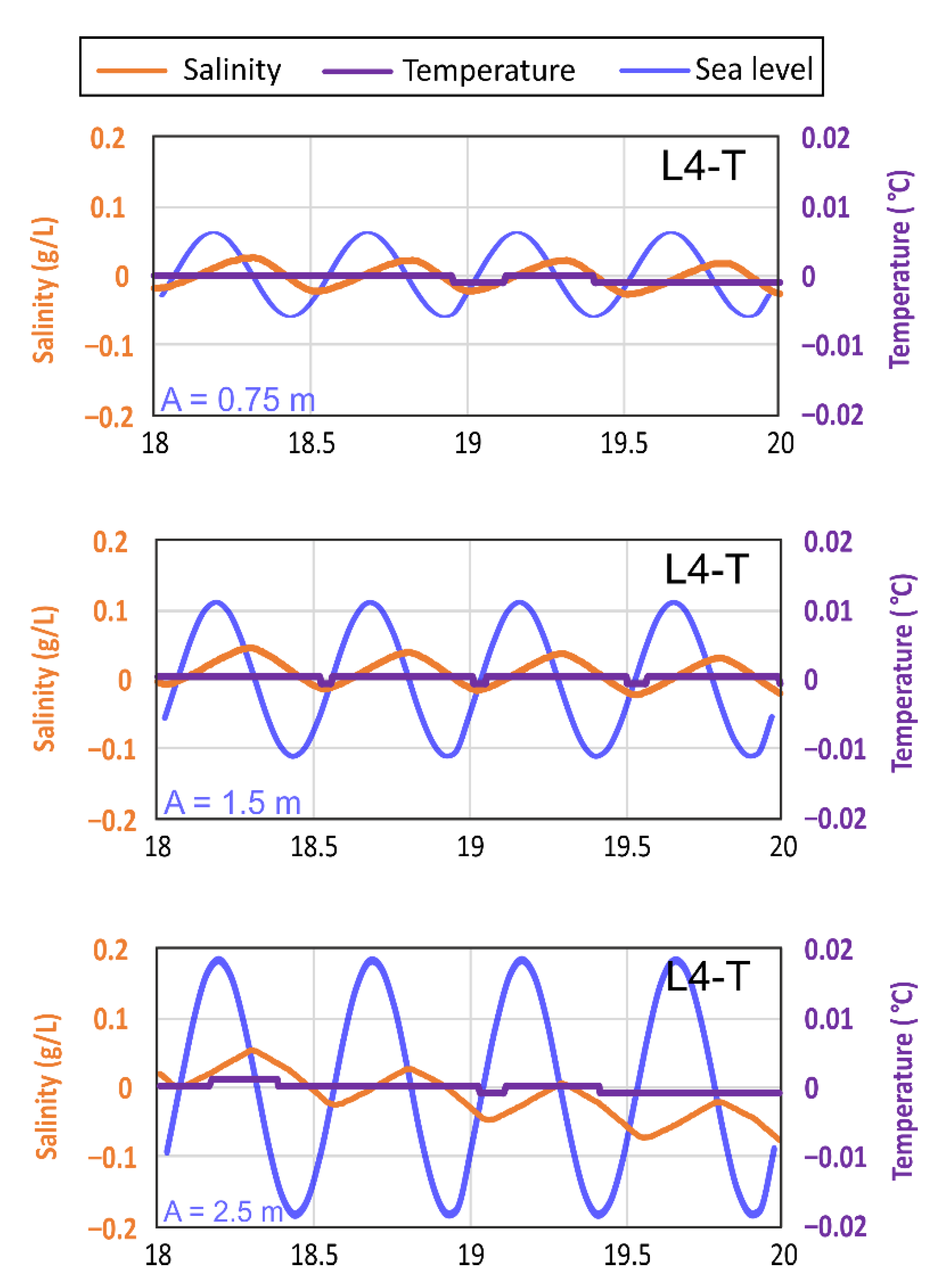
4.4. Numerical Model Results
4.4.1. Model A
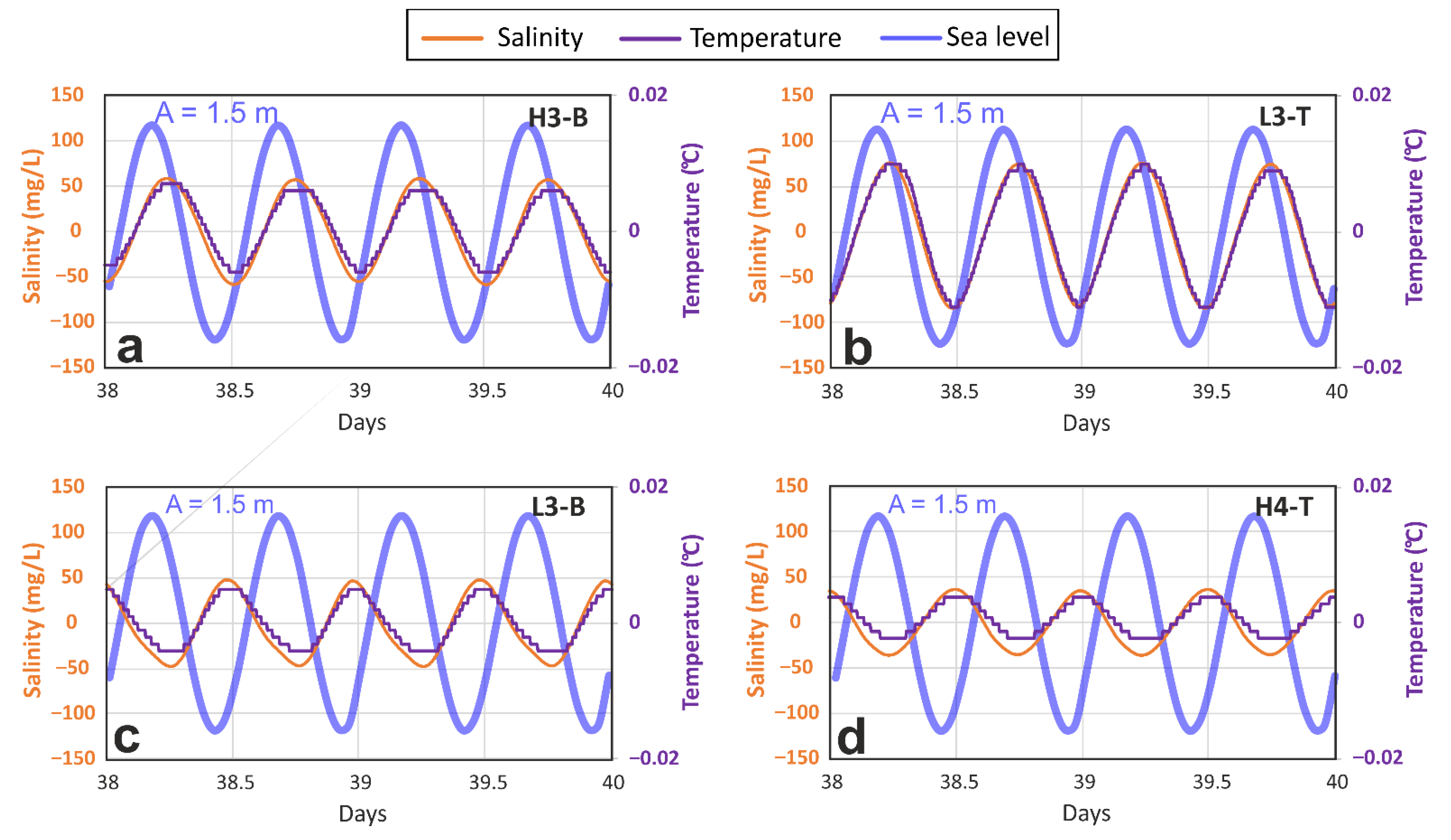
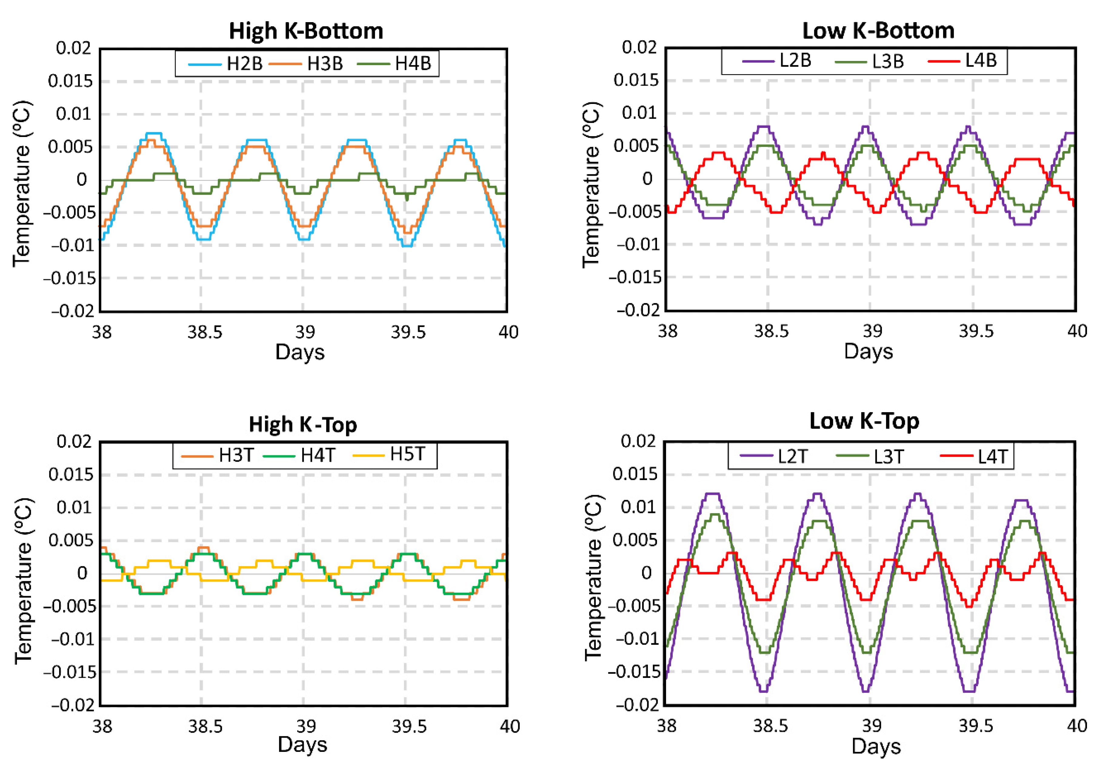
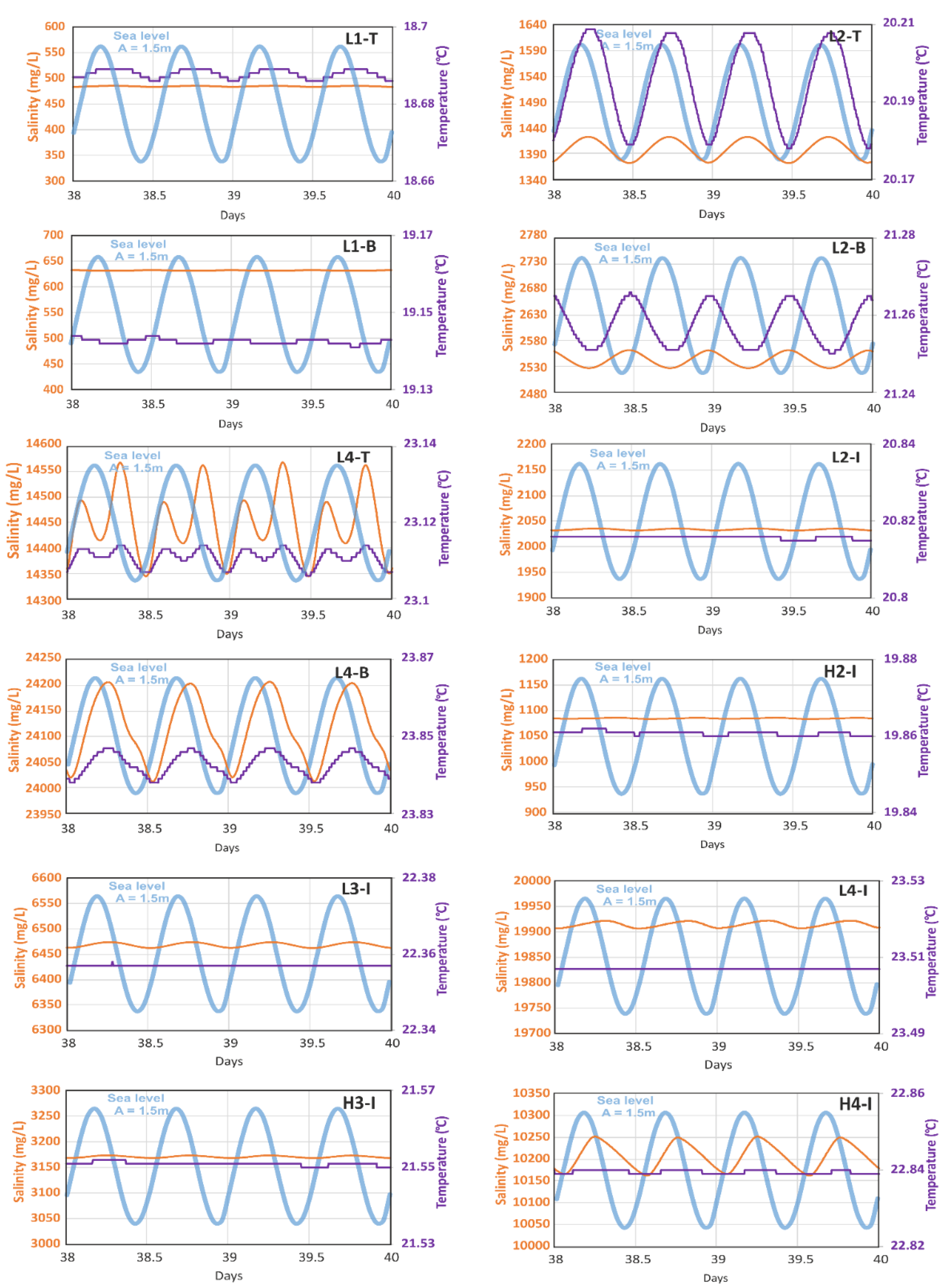
4.4.2. Model B
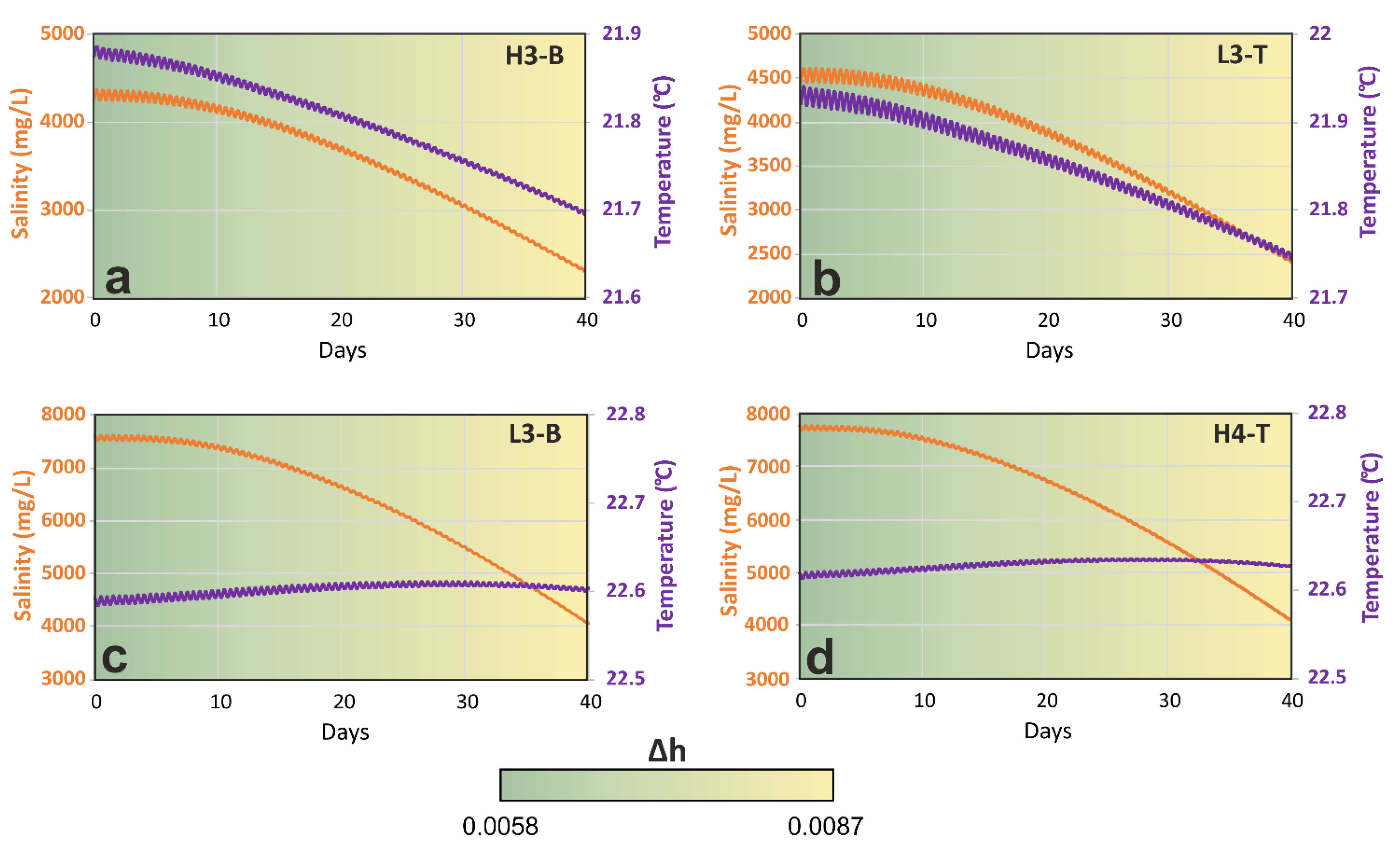
4.4.3. Model C
5. Discussion
6. Conclusions
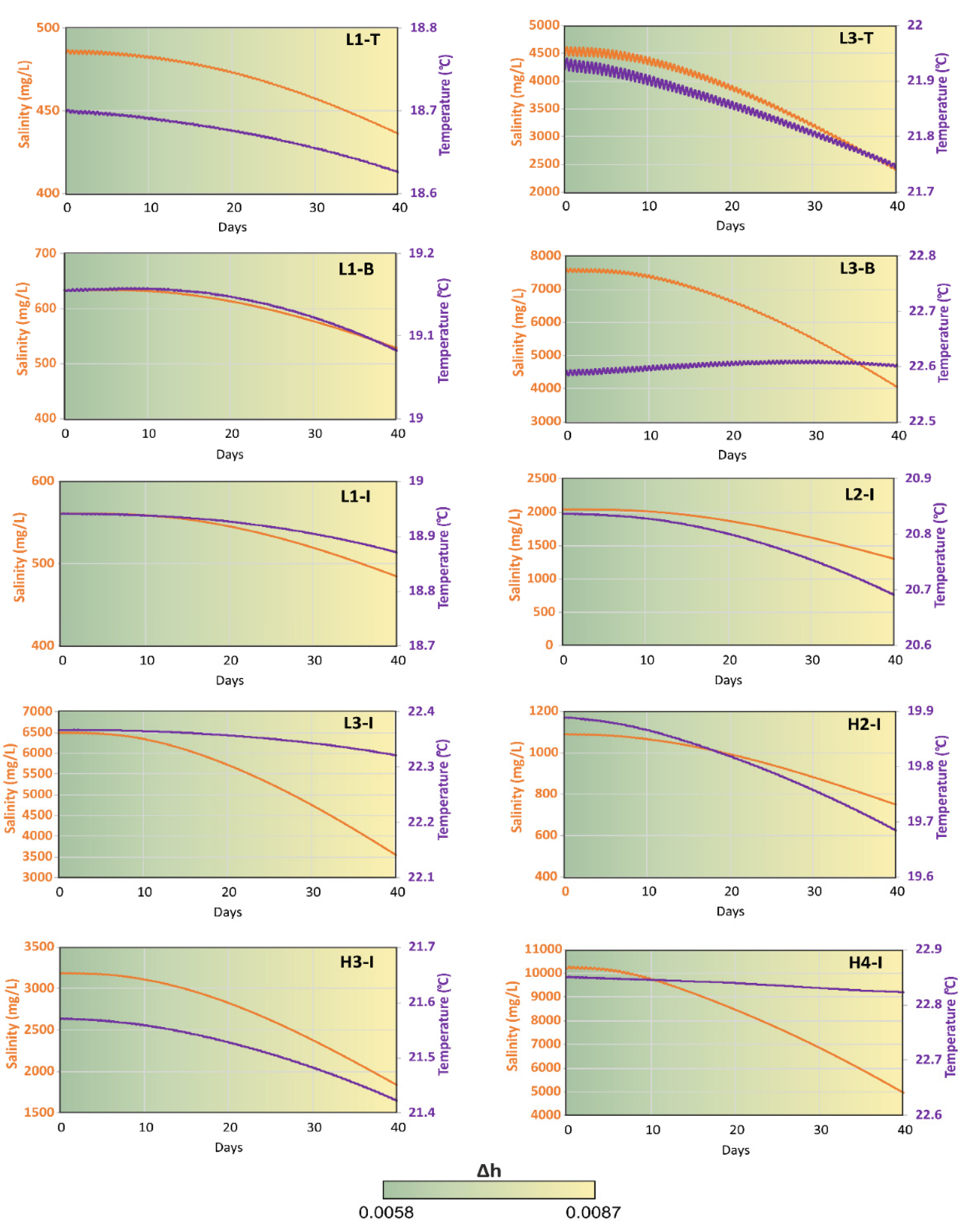
- Seasonal variations of aquifer recharge and sea tides produced a displacement of the fresh groundwater and the FSI and, consequently, changes in EC and temperature distribution. EC fluctuations depended on the horizontal gradient of salinity in the proximity of the FSI. However, the oscillations of temperature depended on the presence of the thermal plume generated by the upwelling flow along the FSI, which was also displaced together with the FSI.
- The amplitude of EC and temperature oscillations associated with sea tides decreased with depth and increased in the areas where hydraulic conductivity changed. The convective heat transport was refracted at the interface between layers with different hydraulic conductivity, inducing a bending with different degrees of inclination (verticality) of the thermal contours. The desynchronization of the oscillations registered at the bottom and at the top of the same layer was produced by the variations in verticality of the thermal plume and the FSI.
- EC and temperature fluctuations were related to hydraulic gradient variations and, hence, to groundwater recharge. The presence of the thermal plume induced a different evolution of salinity and temperature. Salinity progressively decreased as the hydraulic gradient increased. However, the evolution of temperature depended on the position of the observation point with respect to the thermal plume.
- The temperature distribution in coastal aquifers is highly sensitive to natural changes or those induced by humans. The position of the FSI and the thermal plume are dependent on groundwater recharge, which, in turn, depends on climate variability and/or water management. Groundwater recharge plays an important role in the amplitudes of temperature oscillations induced by the tides.
Author Contributions
Funding
Data Availability Statement
Acknowledgments
Conflicts of Interest
Appendix A

Appendix B

References
- Nielsen, P. Tidal dynamics of the water table in beaches. Water Resour. Res. 1990, 26, 2127–2134. [Google Scholar] [CrossRef]
- Li, L.; Barry, D.A.; Stagnitti, F.; Parlange, J.Y.; Jeng, D.S. Beach water table fluctuations due to spring-neap tides: Moving boundary effects. Adv. Water Res. 2000, 23, 817–824. [Google Scholar] [CrossRef]
- Rotzoll, K.; Gingerich, S.B.; Jenson, J.W.; El-Kadi, A.I. Estimating hydraulic properties from tidal attenuation in the Northern Guam Lens Aquifer, territory of Guam, USA. Hydrogeol. J. 2013, 21, 643–654. [Google Scholar] [CrossRef]
- Xun, Z.; Chao, S.; Ting, L.; Ruige, C.; Huan, Z.; Jingbo, Z.; Qin, C. Estimation of aquifer parameters using tide-induced groundwater level measurements in a coastal confined aquifer. Environ. Earth Sci. 2015, 73, 2197–2204. [Google Scholar] [CrossRef]
- Pawlowicz, R.; Beardsley, B.; Lentz, S. Classical tidal harmonic analysis including error estimates in MATLAB using T_TIDE. Comput. Geoscien. 2002, 28, 929–937. [Google Scholar] [CrossRef]
- Levanon, E.; Yechieli, Y.; Shalev, E.; Friedman, V.; Gvirtzman, H. Reliable monitoring of the transition zone between fresh and saline waters in coastal aquifers. Groundw. Monitor. Remed. 2013, 33, 101–110. [Google Scholar] [CrossRef]
- Sánchez-Úbeda, J.P.; Calvache, M.L.; López-Chicano, M.; Duque, C. The Effects of Non-TIDAL Components, Depth of Measurement and the Use of Peak Delays in the Application of Tidal Response Methods. Water Res. Manag. 2018, 32, 481–495. [Google Scholar] [CrossRef]
- Carr, P.A.; Van der Kamp, G. Determining aquifer characteristics by the tidal methods. Water Resour. Res. 1969, 5, 1023–1031. [Google Scholar] [CrossRef]
- Erskine, A.D. The Effect of Tidal Fluctuation on a Coastal Aquifer in the UK. Groundwater 1991, 29, 556–562. [Google Scholar] [CrossRef]
- Raubenheimer, B.; Guza, R.T.; Elgar, S. Tidal Water Table Fluctuations in a Sandy Ocean Beach. Water Resour. Res. 1999, 35, 2313–2320. [Google Scholar] [CrossRef]
- Robinson, M.A.; Gallagher, D.; Reay, W. Field observations of tidal and seasonal variations in groundwater discharge to tidal estuarine surface water. Groundw. Monitor Remed. 1998, 18, 83–92. [Google Scholar] [CrossRef]
- Urish, D.W.; McKenna, T.E. Tidal Effects on Ground Water Discharge through a Sandy Marine Beach. Groundwater 2004, 42, 971–982. [Google Scholar] [CrossRef]
- Heiss, J.W.; Michael, H.A. Saltwater-freshwater mixing dynamics in a sandy beach aquifer over tidal, spring-neap, and seasonal cycles. Water Resour. Res. 2014, 50, 6747–6766. [Google Scholar] [CrossRef]
- Ataie-Ashtiani, B.; Volker, R.E.; Lockington, D.A. Tidal Effects on Sea Water Intrusion in Unconfined Aquifers. J. Hydrol. 1999, 216, 17–31. [Google Scholar] [CrossRef]
- La Licata, I.; Langevin, C.D.; Dausman, A.M.; Alberti, L. Effect of tidal fluctuations on transient dispersion of simulated contaminant concentrations in coastal aquifers. Hydrogeol. J. 2011, 19, 1313–1322. [Google Scholar] [CrossRef]
- Robinson, C.; Li, L.; Barry, D.A. Effect of Tidal Forcing on a Subterranean Estuary. Adv. Water Resour. 2007, 30, 851–865. [Google Scholar] [CrossRef]
- Pool, M.; Post, V.E.A.; Simmons, C.T. Effects of Tidal Fluctuations on Mixing and Spreading in Coastal Aquifers: Homogeneous Case. Water Resour. Res. 2014, 50, 6910–6926. [Google Scholar] [CrossRef]
- Levanon, E.; Yechieli, Y.; Gvirtzman, H.; Shalev, E. Tide-Induced Fluctuations of Salinity and Groundwater Level in Unconfined Aquifers—Field Measurements and Numerical Model. J. Hydrol. 2017, 551, 665–675. [Google Scholar] [CrossRef]
- Yu, X.; Xin, P.; Wang, S.S.J.; Shen, C.; Li, L. Effects of Multi-Constituent Tides on a Subterranean Estuary. Adv. Water Resour. 2019, 124, 53–67. [Google Scholar] [CrossRef]
- Pollock, L.W.; Hummon, W.D. Cyclic Changes in Interstitial Water Content, Atmospheric Exposure, and Temperature in a Marine Beach. Limnol. Oceanogr. 1971, 16, 522–535. [Google Scholar] [CrossRef]
- Li, L.; Horn, D.P.; Baird, A.J. Tide-induced variations in surface temperature and water-table depth in the intertidal zone of a sandy beach. J. Coast. Res. 2006, 22, 1370–1381. [Google Scholar] [CrossRef]
- Vandenbohede, A.; Lebbe, L. Heat transport in a coastal groundwater flow system near De Panne, Belgium. Hydrogeol. J. 2011, 19, 1225–1238. [Google Scholar] [CrossRef]
- Geng, X.; Boufadel, M. Spectral responses of gravel beaches to tidal signals. Sci. Rep. 2017, 7, 40770. [Google Scholar] [CrossRef] [PubMed]
- Nguyen, T.T.M.; Yu, X.; Pu, L.; Xin, P.; Zhang, C.; Barry, D.A.; Li, L. 2020. Effects of temperature on tidally influenced coastal unconfined aquifers. Water Resour. Res. 2020, 56, e2019WR026660. [Google Scholar] [CrossRef]
- Kim, K.Y.; Chon, C.M.; Park, K.H.; Park, Y.S.; Woo, N.C. Multi-Depth Monitoring of Electrical Conductivity and Temperature of Groundwater at a Multilayered Coastal Aquifer: Jeju Island, Korea. Hydrol. Process. 2008, 22, 3724–3733. [Google Scholar] [CrossRef]
- Kim, K.Y.; Park, Y.S.; Kim, G.P.; Park, K.H. Dynamic Freshwater-Saline Water Interaction in the Coastal Zone of Jeju Island, South Korea. Hydrogeol. J. 2009, 17, 617–629. [Google Scholar] [CrossRef]
- Vallejos, A.; Sola, F.; Pulido-Bosch, A. Processes Influencing Groundwater Level and the Freshwater-Saltwater Interface in a Coastal Aquifer. Water Res. Manag. 2015, 29, 679–697. [Google Scholar] [CrossRef]
- Blanco-Coronas, A.M.; Duque, C.; Calvache, M.L.; López-Chicano, M. Temperature Distribution in Coastal Aquifers: Insights from Groundwater Modeling and Field Data. J. Hydrol. 2021, 603, 126912. [Google Scholar] [CrossRef]
- Anderson, M.P. Heat as a ground water tracer. Groundwater 2005, 43, 951–968. [Google Scholar] [CrossRef]
- Del Val, L. Advancing in the Characterization of Coastal Aquifers: A Multimethodological Approach Based on Fiber Optics Distributed Temperature Sensing. Ph.D. Thesis, Polytechnic University of Catalonia, Barcelona, Spain, 2020. [Google Scholar]
- Taniguchi, M. Evaluations of the saltwater-groundwater interface from borehole temperature in a coastal region. Geophys. Res. Lett. 2000, 27, 713–716. [Google Scholar] [CrossRef]
- Fidelibus, M.D.; Pulido-Bosch, A. Groundwater temperature as an indicator of the vulnerability of Karst coastal aquifers. Geosciences 2019, 9, 23. [Google Scholar] [CrossRef]
- LeRoux, N.K.; Kurylyk, B.L.; Briggs, M.A.; Irvine, D.J.; Tamborski, J.J.; Bense, V.F. Using Heat to Trace Vertical Water Fluxes in Sediment Experiencing Concurrent Tidal Pumping and Groundwater Discharge. Water Resour. Res. 2021, 57, e2020WR027904. [Google Scholar] [CrossRef]
- Parsons, M.L. Groundwater thermal regime in a glacial complex. Water Resour. Res. 1970, 6, 1701–2172. [Google Scholar] [CrossRef]
- Kurylyk, B.L.; Irvine, D.J.; Bense, V.F. Theory, tools, and multidisciplinary applications for tracing groundwater fluxes from temperature profiles. Wires Water 2019, 6, e1329. [Google Scholar] [CrossRef]
- Tóth, J. A theory of groundwater motion in small basins in central Alberta. Canada. J. Geophys. Res. 1962, 67, 4375–43787. [Google Scholar] [CrossRef]
- Domenico, P.A.; Palciauskas, V.V. Theoretical analysis of forced convective heat transfer in regional groundwater flow. GSA Bull. 1973, 84, 3803–3814. [Google Scholar] [CrossRef]
- An, R.; Jiang, X.W.; Wang, J.Z.; Wan, L.; Wang, X.S.; Li, H. A theoretical analysis of basin-scale groundwater temperature distribution. Hydrogeol. J. 2015, 23, 397–404. [Google Scholar] [CrossRef]
- Szijártó, M.; Galsa, A.; Tóth, Á.; Mádl-Szőnyi, J. Numerical investigation of the combined effect of forced and free thermal convection in synthetic groundwater basins. J. Hydrol. 2019, 572, 364–379. [Google Scholar] [CrossRef]
- Befus, K.M.; Cardenas, M.B.; Erler, D.V.; Santos, I.R.; Eyre, B.D. Heat transport dynamics at a sandy intertidal zone. Water Resour. Res. 2013, 49, 3770–3786. [Google Scholar] [CrossRef]
- Tirado-Conde, J.; Engesgaard, P.; Karan, S.; Müller, S.; Duque, C. Evaluation of temperature profiling and seepage meter methods for quantifying submarine groundwater discharge to coastal lagoons: Impacts of saltwater intrusion and the associated thermal regime. Water 2019, 11, 1648. [Google Scholar] [CrossRef] [Green Version]
- Duque, C.; Calvache, M.L.; Pedrera, A.; Martín-Rosales, W.; López-Chicano, M. Combined time domain electromagnetic soundings and gravimetry to determine marine intrusion in a detrital coastal aquifer (Southern Spain). J. Hydrol. 2008, 349, 536–547. [Google Scholar] [CrossRef]
- Calvache, M.L.; Ibáñez, S.; Duque, C.; Martín-Rosales, W.; López-Chicano, M.; Rubio, J.C.; González, A.; Viseras, C. Numerical modelling of the potential effects of a dam on a coastal aquifer in S. Spain. Hydrol. Process. 2009, 23, 1268–1281. [Google Scholar] [CrossRef]
- Duque, C. Influencia Antrópica Sobre la Hidrogeología del Acuífero Motril-Salobreña. Ph.D. Thesis, University of Granada, Granada, Spain, 2009. [Google Scholar]
- Duque, C.; Calvache, M.L.; Engesgaard, P. Investigating river-aquifer relations using water temperature in an anthropized environment (Motril-Salobreña aquifer). J. Hydrol. 2010, 381, 121–133. [Google Scholar] [CrossRef]
- Blanco-Coronas, A.M.; López-Chicano, M.; Acosta-Rodriguez, R.; Calvache, M.L. Groundwater recharge-discharge estimation with differential flow gaugings in the final stretch of the Guadalfeo river (Granada). Geogaceta 2021, 69, 91–94. [Google Scholar]
- Duque, C.; López-Chicano, M.; Calvache, M.L.; Martín-Rosales, W.; Gómez-Fontalva, J.M.; Crespo, F. Recharge sources and hydrogeological effects of irrigation and an influent river identified by stable isotopes in the Motril-Salobreña aquifer (Southern Spain). Hydrol. Process. 2011, 25, 2261–2274. [Google Scholar] [CrossRef]
- Olsen, J.T. Modeling the Evolution of Salinity in the Motril-Salobreña Aquifer Using a Paleo-Hydrogeological Model. Master’s Thesis, University of Oslo, Oslo, Norway, 2016. [Google Scholar]
- Calvache, M.L.; Duque, C.; Gómez-Fontalva, J.M.; Crespo, F. Processes affecting groundwater temperature patterns in a coastal aquifer. Int. J. Environ. Sci. Technol. 2011, 8, 223–236. [Google Scholar] [CrossRef]
- Calvache, M.L.; Sánchez-Úbeda, J.P.; Duque, C.; López-Chicano, M.; De La Torre, B. Evaluation of analytical methods to study aquifer properties with pumping tests in coastal aquifers with numerical modelling (Motril-Salobreña aquifer). Water Resour. Manag. 2015, 30, 559–575. [Google Scholar] [CrossRef]
- Sánchez-Úbeda, J.P.; Calvache, M.L.; Duque, C.; López-Chicano, M. Filtering methods in tidal-affected groundwater head measurements: Application of harmonic analysis and continuous wavelet transform. Adv. Water Res. 2016, 97, 52–72. [Google Scholar] [CrossRef]
- Pan, H.; Lv, X.; Wang, Y.; Matte, P.; Chen, H.; Jin, G. Exploration of Tidal-Fluvial Interaction in the Columbia River Estuary Using S_TIDE. J. Geophys. Res. Ocean. 2018, 123, 6598–6619. [Google Scholar] [CrossRef]
- Shumway, H.S.; Stoffer, D.S. Time Series Analysis and its Applications: With R Examples, 2nd ed.; Springer Science + Business Media, LLC.: New York, NY, USA, 2006; 575p. [Google Scholar]
- Larocque, M.; Mangin, A.; Razack, M.; Banton, O. Contribution of correlation and spectral analyses to the regional study of a large karst aquifer (Charente, France). J. Hydrol. 1998, 205, 217–231. [Google Scholar] [CrossRef]
- Padilla, A.; Pulido-Bosch, A. Study of hydrographs of karstic aquifers by means of correlation and cross-spectral analysis. J. Hydrol. 1995, 168, 73–89. [Google Scholar] [CrossRef]
- Langevin, C.D.; Thorne, D.T.; Dausman, A.M.; Sukop, M.C.; Guo, W. SEAWAT Version 4: A Computer Program for Simulation of Multi-Species Solute and Heat Transport; U.S. Geological Survey Techniques and Methods; Geological Survey (U.S.): Reston, VA, USA, 2008; Chapter A22.
- Harbaugh, A.W.; Banta, E.R.; Hill, M.C.; Mcdonald, M.G. MODFLOW-2000, The U.S. Geological Survey Modular Ground-Water Model User Guide to Modularization Concepts and the Ground-Water Flow Process, Geological Survey; CO McDonald Morrissey Associates: Concord, NH, USA, 2000. [Google Scholar]
- Zheng, C.; Wang, P.P. MT3DMS—A Modular Three-Dimensional Multispecies Transport Model for Simulation of Advection, Dispersion and Chemical Reactions of Contaminants in Groundwater Systems: Documentation and User’s Guide; U.S. Army Corps of Engineers: Washington, DC, USA, 1999.
- Yang, X.; Shaoa, Q.; Hoteit, H.; Carrera, J.; Younes, A.; Fahs, M. Three-dimensional natural convection, entropy generation and mixing in heterogeneous porous medium. Adv. Water Resour. 2021, 115, 103992. [Google Scholar] [CrossRef]
- Tabrizinejadas, S.; Fahs, M.; Ataie-Ashtiani, B.; Simmons, C.T.; di Chiara Roupert, R.; Younes, A. A Fourier series solution for transient three-dimensional thermohaline convection in porous enclosures. Water Resour. Res. 2020, 56, e2020WR028111. [Google Scholar] [CrossRef]
- Stauffer, F.; Bayer, P.; Blum, P.; Giraldo, N.; Kinzelbach, W. Thermal Use of Shallow Groundwater; CRC Press: Boca Raton, FL, USA, 2014. [Google Scholar] [CrossRef]
- Xiaoqing, S.; Ming, J.; Peiwen, X. Analysis Of The Thermophysical Properties And Influencing Factors Of Various Rock Types From The Guizhou Province. EDP Sciences. E3S Web Conf. 2018, 53, 03059. [Google Scholar] [CrossRef]
- Pugh, D.T. Tides, Purges and Mean Sea Level; John Wiley & Sons Ltd.: Chichester, UK, 1996. [Google Scholar]
- Saar, M.O. Review: Geothermal heat as a tracer of large-scale groundwater flow and as a means to determine permeability fields. Hydrogeol. J. 2011, 19, 31–52. [Google Scholar] [CrossRef]
- Wang, Z.; Gao, P.; Jiang, G.; Wang, Y.; Hu, S. Heat Flow Correction for the High-Permeability Formation: A Case Study for Xiong’an New Area. Lithosphere 2021, 5, 9171191. [Google Scholar] [CrossRef]
- Ma, J.; Zhou, Z. Origin of the low-medium temperature hot springs around Nanjing, China. Open Geosci. 2021, 13, 820–834. [Google Scholar] [CrossRef]
- Levanon, E.; Shalev, E.; Yechieli, Y.; Gvirtzman, H. Advances in Water Resources Fluctuations of fresh-saline water interface and of water table induced by sea tides in unconfined aquifers. Adv. Water Resour. 2016, 96, 34–42. [Google Scholar] [CrossRef]
- Mao, X.; Enot, P.; Barry, D.A.; Li, L.; Binley, A.; Jeng, D.S. Tidal influence on behaviour of a coastal aquifer adjacent to a low-relief estuary. J. Hydrol. 2006, 327, 110–127. [Google Scholar] [CrossRef]
- Costall, A.R.; Harris, B.D.; Teo, B.; Schaa, R.; Wagner, F.M.; Pigois, J.P. Groundwater Throughflow and Seawater Intrusion in High Quality Coastal Aquifers. Sci. Rep. 2020, 10, 9866. [Google Scholar] [CrossRef]


| Input Parameters | Value | Source |
|---|---|---|
| Specific storage | 1 × 10⁻⁵ m−1 | Calvache et al. [50] |
| Specific yield | 0.25 | Similar value to Calvache et al. [50] |
| 0.3 | Duque et al. [42] | |
| Longitudinal dispersivity | 20 m | Stauffer et al. [61] |
| Vertical transverse dispersivity | 10 m | Stauffer et al. [61] |
| 1 × 10⁻¹⁰ m2/d | Langevin et al. [56] | |
| 0.58 W/m °C | Langevin et al. [56] | |
| 2.9 W/m °C | Approximate value for gravel [62] | |
| 4186 J/kg °C | Langevin et al. [56] | |
| 830 J/kg °C | Approximate value for gravel [62] | |
| 0.15 m2/d | Langevin et al. [56] | |
| 1.8 W/m °C | Langevin et al. [56] | |
| 2 × 10⁻⁷ L/mg | Langevin et al. [56] | |
| Density change with concentration | 0.7 | Langevin et al. [56] |
| Density change with temperature | −0.375 kg/(m3 °C) | Langevin et al. [56] |
| Density vs pressure head slope | 0.00446 kg/m4 | Langevin et al. [56] |
| 1800 kg/m3 | ||
| Reference temperature | 25 °C | Langevin et al. [56] |
| Viscosity vs concentration slope | 1.923 × 10⁻⁶ m4/d | Langevin et al. [56] |
| Reference viscosity | 86.4 kg/ m d | Langevin et al. [56] |
| L1-T | L1-B | H2-T | H2-I | H2-B | L2-T | L2-B | H3-T | H3-I | H3-B |
|---|---|---|---|---|---|---|---|---|---|
| −20 m | −31 m | −34 m | −70 m | −79 m | −88 m | −96 m | −97 m | −110 m | −122 m |
| L3-T | L3-I | L3-B | H4-T | H4-I | H4-B | L4-T | L4-I | L4-B | H5-T |
| −124 m | −131 m | −139 m | −140 m | −155 m | −168 m | −169 m | −175 m | −182 m | −183 m |
| Harmonic Constituent | Symbol | Amplitude (m) | Amplitude (°C) | ||
|---|---|---|---|---|---|
| Sea Level | S-3 | S-4 | S-5 | ||
| Lunisolar synodic fortnightly | Msf | 0.046 | 0.003 | 0.007 | 0.012 |
| Principal lunar diurnal | O1 | 0.022 | 0.004 | 0.001 | 0.005 |
| Luni-solar diurnal | K1 | 0.029 | 0.004 | 0.001 | 0.006 |
| Lunar diurnal | OO1 | 0.013 | 0.001 | 0.002 | 0.001 |
| Larger lunar elliptic semidiurnal | N2 | 0.031 | 0.004 | 0.002 | 0.006 |
| Principal lunar semidiurnal | M2 | 0.157 | 0.021 | 0.009 | 0.027 |
| Principal solar semidiurnal | S2 | 0.064 | 0.008 | 0.003 | 0.011 |
| Shallow water overtides of principal lunar constituent | M4 | 0.016 | 0.001 | 0 | 0 |
| Depth | Amplitude (°C) | Range (°C) | |||
|---|---|---|---|---|---|
| 132 m | 6.4 | 6.1 | −1.1 | 0.04 | 17.7–17.8 |
| 217 m | 5.6 | 5.6 | - | 0.02 | 18.9–19.0 |
| 236 m | 5.4 | 5.3 | −0.7 | 0.06 | 19.9–20.0 |
Publisher’s Note: MDPI stays neutral with regard to jurisdictional claims in published maps and institutional affiliations. |
© 2022 by the authors. Licensee MDPI, Basel, Switzerland. This article is an open access article distributed under the terms and conditions of the Creative Commons Attribution (CC BY) license (https://creativecommons.org/licenses/by/4.0/).
Share and Cite
Blanco-Coronas, A.M.; Calvache, M.L.; López-Chicano, M.; Martín-Montañés, C.; Jiménez-Sánchez, J.; Duque, C. Salinity and Temperature Variations near the Freshwater-Saltwater Interface in Coastal Aquifers Induced by Ocean Tides and Changes in Recharge. Water 2022, 14, 2807. https://doi.org/10.3390/w14182807
Blanco-Coronas AM, Calvache ML, López-Chicano M, Martín-Montañés C, Jiménez-Sánchez J, Duque C. Salinity and Temperature Variations near the Freshwater-Saltwater Interface in Coastal Aquifers Induced by Ocean Tides and Changes in Recharge. Water. 2022; 14(18):2807. https://doi.org/10.3390/w14182807
Chicago/Turabian StyleBlanco-Coronas, Angela M., Maria L. Calvache, Manuel López-Chicano, Crisanto Martín-Montañés, Jorge Jiménez-Sánchez, and Carlos Duque. 2022. "Salinity and Temperature Variations near the Freshwater-Saltwater Interface in Coastal Aquifers Induced by Ocean Tides and Changes in Recharge" Water 14, no. 18: 2807. https://doi.org/10.3390/w14182807