
The Future Change in Evaporation Based on the CMIP6 Merged Data Generated by Deep-Learning Method in China

1
Beijing Institute of Meteorological Applications, Beijing 100029, China
2
National Key Laboratory of Geographic Information Engineering, Xi’an 710054, China
3
School of Geographical Science, Nanjing University of Information Science and Technology (NUIST), Nanjing 210044, China
4
School of Computer Science, Nanjing University of Information Science and Technology (NUIST), Nanjing 210044, China
*
Author to whom correspondence should be addressed.
Water 2022, 14(18), 2800; https://doi.org/10.3390/w14182800
Submission received: 25 June 2022
/
Revised: 28 August 2022
/
Accepted: 5 September 2022
/
Published: 8 September 2022
(This article belongs to the Topic Recent Advances in Hydroinformatics: Focusing on Machine Learning and Remote Sensing in Hydrology)
Abstract
:Land evaporation (LET) is an important variable in climate change, water cycle and water resources management. Mastering the projected changes in LET is significant for crop water requirements and the energy cycle. The global climate model (GCM) is a vital tool for future climate change research. However, the GCMs have low spatial resolution and relatively high errors. We use a deep learning (DL)-based model to deal with this problem. The DL approach can downscale the model data and merge simultaneously. We applied the DL approach to a suit of models from the Coupled Model Intercomparison Project 6th edition (CMIP6) LET data. From the result of all the evaluation metrics, the DL merged data greatly improved in both spatial and time dimensions. The mean RMSE is 5.85 mm and the correlation is 0.95 between the DL merged data and reference data (historical reliable evaporation data). The future LET evidently increases in four scenarios (SSP1–2.6, SSP2–4.5, SSP3–7.0, and SSP5–8.5), and the upward intensity rises from the low to high emission scenarios. The highest increasing regions are in the Tibet Plateau and the south of China and the trend is larger than 10 mm/decade in the high scenarios. From the seasonal point of view, the increasing trend in spring and summer is far larger than for autumn and winter. The Tibet Plateau and the northeast of China have the largest upward trend in the spring of SSP5–8.5, higher than 1.6 mm/decade.
1. Introduction
The Sixth Assessment Report of the Intergovernmental Panel on Climate Change (IPCC) states that global warming caused by greenhouse gases is evidently increasing. Global warming seriously impacts the water cycle and resources [1,2]. Land evaporation (LET) plays a significant role in the water cycle and water resource management [3] and is also one of the key variables in the soil-vegetation-atmosphere system [4]. Because the interaction between meteorological factors is complex, many factors influence the ET change [5]. It is important to understand the spatial-temporal variation in LET under climate change. Accurately grasping the future changes in LET is crucial to understanding the response mechanism of hydrological processes to climate change.
The long time LET data recorded by the meteorological stations and those from satellite retrievals are rather short and cannot be used for meaningful historical changes and projections. The Global Climate Models (GCM) of the coupled model inter-comparison project (CMIP) are vital tools to understand the influence of future climate change on the water cycle [6]. Because more scientific problems need to be handled, CMIP is continuing to revise the new GCM [7]. The new version of CMIP6 is a combination of the representative concentrations pathway (RCPs) in the CMIP5 and the shared socioeconomic pathway (SSP) [8]. CIMP6 has five SSPs, representing different social development degrees [9,10,11,12,13]. Compared with the CMIP5, CMIP6 has more models and experiments with widespread improvement in many fields, such as spatial resolution, physical parameterizations, etc. [7]. These new version GCMs can help us understand the future climate change better.
Most studies use the GCM data to research future climate changes, influences, and sensitivities [14,15]. However, different variables of GCM are subjected to some uncertainties and sensitivities due to the climate system’s internal changes and model physics algorithms [16,17,18]. Based on the assessment result with the CMIP6 model, a conclusion can be drawn that no single model performs best in different regions for any of the evaluation methods [19]. So, we need to consider how to merge the GCM data scientifically. For this problem, the multi-model ensemble mean (MME) method is a common, easy, and effective method [20]. The MME method still has some shortcomings; for example, this method is easily affected by extreme values and reduces the simulation performance in some local regions.
Although the spatial resolution of GCM has improved in the CMIP6, the resolution of GCM still cannot satisfy the requirement for detailed regional-scale research [21]. Spatial downscaling methods have been widely used for the data downscaling of GCM. The refinement methods of the GCM mainly include statistical downscaling [22] and dynamic downscaling [23]. The dynamic downscaling calculation is complex and uses the high-resolution regional climate model (RCM), but it can provide higher resolution downscaling data [24,25,26]. Although the satistical downscaling calculation is simple, its downscaling performance highly depends on the quantity and quality of regional meteorological data [27]. The statistic downscaling method builds the relationship between the GCM and the local-scale meteorological data and then generates high-resolution data. The common statistical downscaling techniques are regression-based, such as generalized linear regression models and those reported in [28,29]. Both methods can improve data resolution, but there is still a large deviation compared with the observation data [30]. Many bias correction methods are proposed to deal with this problem of GCM, such as statistics based on the mean, variance, and standard deviation [31,32], probability distribution-based bias correction [33], etc. However, the current GCM deviation correction methods have some limitations (such as GCM average deviation correction only considers the GCM average deviation and quantile-quantile correction also brings additional deviation to the spatial gradient of variables) [34,35]. In addition, most bias correction methods are for a single model dataset, bringing greater uncertainty in predicting the future climate.
However, the above downscaling methods do not have the ability to integrate multi-source data. In recent years, deep learning (DL)-based methods have played an increasingly important role in earth science because of their better ability to deal with big data [36] and have been successfully applied to many areas [37,38,39]. The DL model from the super-resolution (SR) field is suitable for dealing with the data downscaling and data merge problem of GCM. In essence, deep learning is a data fusion and downscaling technology based on a nonlinear relationship. These DL models can input many coarse-resolution GCM LET data to obtain high-resolution LET data, which means that the DL model can learn information from different GCMs and simultaneously perform data fusion and data downscaling, thereby reducing uncertainty. The SR convolutional neural network (SRCNN) outperforms the traditional SR method, which is the pioneer of image super resolution and reconstruction [40]. Subsequently, some DL approaches have been applied to the SR field to improve the performance [41,42]. In previous studies, deep learning has shown a strong ability to downscale meteorological data. For example, Vandal et al. (2017) used a SR convolutional neural network framework stacked with three-layer convolution to downscale precipitation from 1° to 1/8°degrees. The results were far better than the traditional statistical downscaling methods [43]. In another study by Rodrigues et al. (2018), they used the deep learning SR algorithm to significantly improve temperature and precipitation data resolution and ensure accuracy [44]. The deep-learning methods are non-local model output statistics (MOS) methods used to downscale data. Different from other statistical methods, they also consider information from the nearby grid.
The novelty of this work is the data merge and downscaling of GCM that was performed simultaneously with a DL-based model. Unlike the traditional methods, we can input many low resolution LET GCM data and obtain one set of high-resolution LET data; the DL model can learn information from different GCMs and perform data merging and data downscaling simultaneously, and reduce uncertainty. This work uses historical GCM LET to train a DL model and applies this relationship to merge the future data. Our work aims to create high-resolution LET data at 0.25° × 0.25° with high precision. Then, we can use the merged future data in different scenarios (SSP1–2.6, SSP2–45, SSP3–70, and SSP5–8.5) to analyze LET changes in China.
2. Materials and Methods
2.1. Study Region and Data
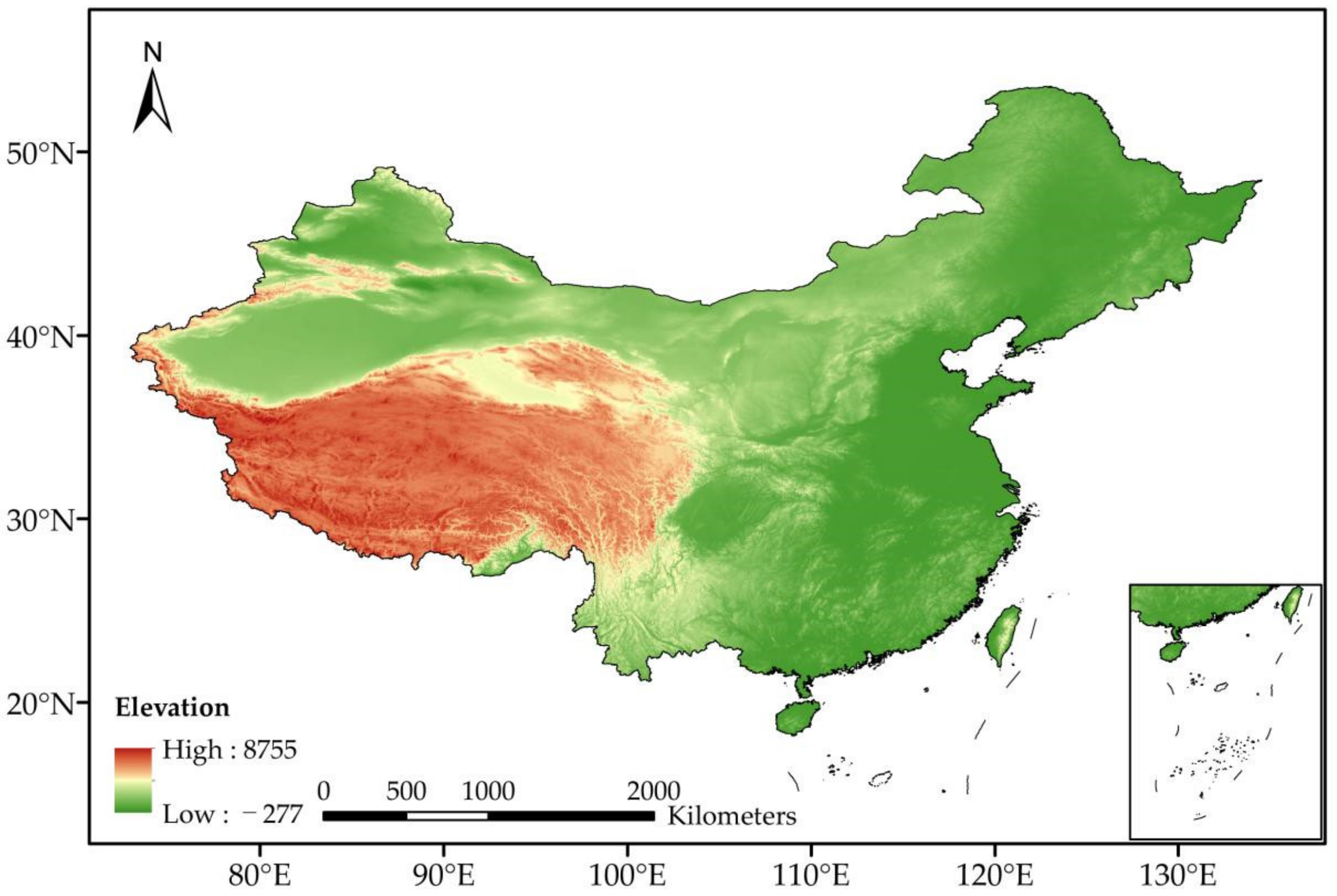
Our study region is China, the third biggest country in the world, with a vast land area of about 9.6 million km2. The climate of the study area is very complex, from the tropical to the temperate zone in China. The terrain of China includes the characteristics of high mountains and plateaus in the west and low terrains in the east. North China is relatively dry arid to semi-arid, and South China is relatively wet to humid. Because the Tibetan Plateau blocks warm and humid air from the Indian Ocean, the drought region in China is usually located in the inland areas. The climate in eastern China is dominated by the East Asian monsoon climate of hot and humid summers and dry and cold winters. The location of our study area is showed in the Figure 1.
2.1.1. Evaporation Reanalysis Data
We use a harmonized evaporation (ET) dataset as the reference data in our work [45]. These data were generated by the reliability ensemble averaging (REA) method with the ERA5, GLDAS, MERRA2, GLEAM3.2a and the flux tower observation data. According to the results, the merged data performed well in the complex vegetation condition. In addition, these data can describe the trend of the evaporation changes in different regions globally. The period of this data is 1980–2017, the temporal resolution is one month and the spatial resolution is 0.25° × 0.25°. We use the RD to represent these data in the following analysis to facilitate expression. These data are available at https://doi.org/10.5281/zenodo.4595941 (accessed on 12 November 2021).
2.1.2. CMIP6 Evaporation Data
This work used 22 monthly ET GCM data from the CMIP6. Those data can be accessed at the https://esgf-node.llnl.gov/projects/cmip6/ (accessed on 12 November 2021). One historical scenario in the period of 1850–2014 and four future scenarios, including SSP1–2.6, SSP2–4.5, SSP3–7.0 and SSP5–8.5, in the period of 2015–2100 were used in this study. Table 1 depicts the GCM information in this work. The spatial resolutions of the raw GCM data are relatively low, ranging from 0.703125° to 2.8125° and the spatial resolutions of most GCMs data are near to 2°. To retain more information from the raw GCM, we resampled all the GCM data to 2° × 2° with the linear interpolation method.
2.2. Methods
2.2.1. Deep-Learning Method
A deep convolution network designed for climate downscaling and fusion named Ynet was used in our work [46]. The Ynet learned from the historical period’s relationship between the RD data and the GCM ET data. In the future stage, we generated the future improved merged data using this relationship. The input data of the Ynet was the 22 GCM raw spatial resolutions with 2° × 2° and the output of the Ynet was one set of high-resolution 0.25° × 0.25° merged data. The Ynet consists of some convolutional/deconvolutional layers, upsampling layers and a fusion layer. The convolutional/deconvolutional layers are in charge of feature extraction, the upsampling layers downscale the GCM data and the fusion layer can merge multiple GCM inputs into one output.
The convolutional and deconvolutional layer have a 3 × 3 kernel size with stride 1, padding 1 and ReLU activation. Figure 1 shows the main structure of the Ynet, including the following three parts: quasisymmetric structure with skip connections, an upsampling part and fusion part. The structure of the first part tackles the gradient vanishing problem and is regarded as the feature extractor, which captures the abstraction of the low resolution. This part has 30 convolutional layers and 15 deconvolutional layers. The purpose of adding a convolutional layer after each deconvolutional layer is to alleviate the checkerboard artifacts caused by the deconvolutional layer. The second part includes an upsampling layer and two convolutional layers, with the same feature depth as the number of input GCM data. This part can downscale the GCM data. The third part is the fusion part; this part merges the downscaled data and outputs one set of high-resolution merged data. The input of the fusion part includes the up-sampling part output, auxiliary data and direct up-sampled GCM data that can help to improve the result. The auxiliary data include the climatological data calculated by RD in our work. The 22 GCM ET data will downscale and merge to one set of resolution data through those three parts of the Ynet.
2.2.2. Evaluation Metric
To comprehensively compare the performance of the DL merged data and the traditional ensemble method, the mean absolute error (MAE), root mean square deviation (RMSE) and unbiased root mean square deviation (ubRMSE) were applied in the subsequent evaluation. We used the mean square error (MSE) in the training process as the loss function to train the Y-net. The coefficient of correction (R) was also used for the evaluation. The formulas of those metrics are as follows:
In the Equations (1)–(5), n represents the number of all samples. Yi is the reference evaporation data and Si is the DL merged data. , represent the mean value of the reference data and DL merged data, respectively.
In addition, we also use the Taylor diagram [47] to evaluate the RD data, DL merged data, MME data and single GCM model. It requires standard deviation (STD), ubRMSD and R.
2.2.3. Training Setting and Strategy
In the evaluated period, a total of 420 months were used for training from 1980 to 2014. The historical data were separated into two datasets with the ratio of 4 to 1, including the training dataset (1980–2007) and test dataset (2008–2014). Those two datasets are independent. The training dataset was used to train the network, tune the parameter, and then choose the best model parameter according to the performance in the test dataset.
In the data preprocessing stage, we scaled all the GCM and RD data to the range of 0–1 by the maximum and minimum normalization method. This operation can accelerate network convergence. In the training process, we applied a land-ocean mask to help the DL model pay more attention to the land region to improve the result. One epoch means that the model iterate all the data and 100 epochs were used in the training phase. The initial learning rate was 1 × 10⁻⁴ and the batch size was 1 in the hyper parameter set.
3. Results
3.1. Evaluation of Merged Data
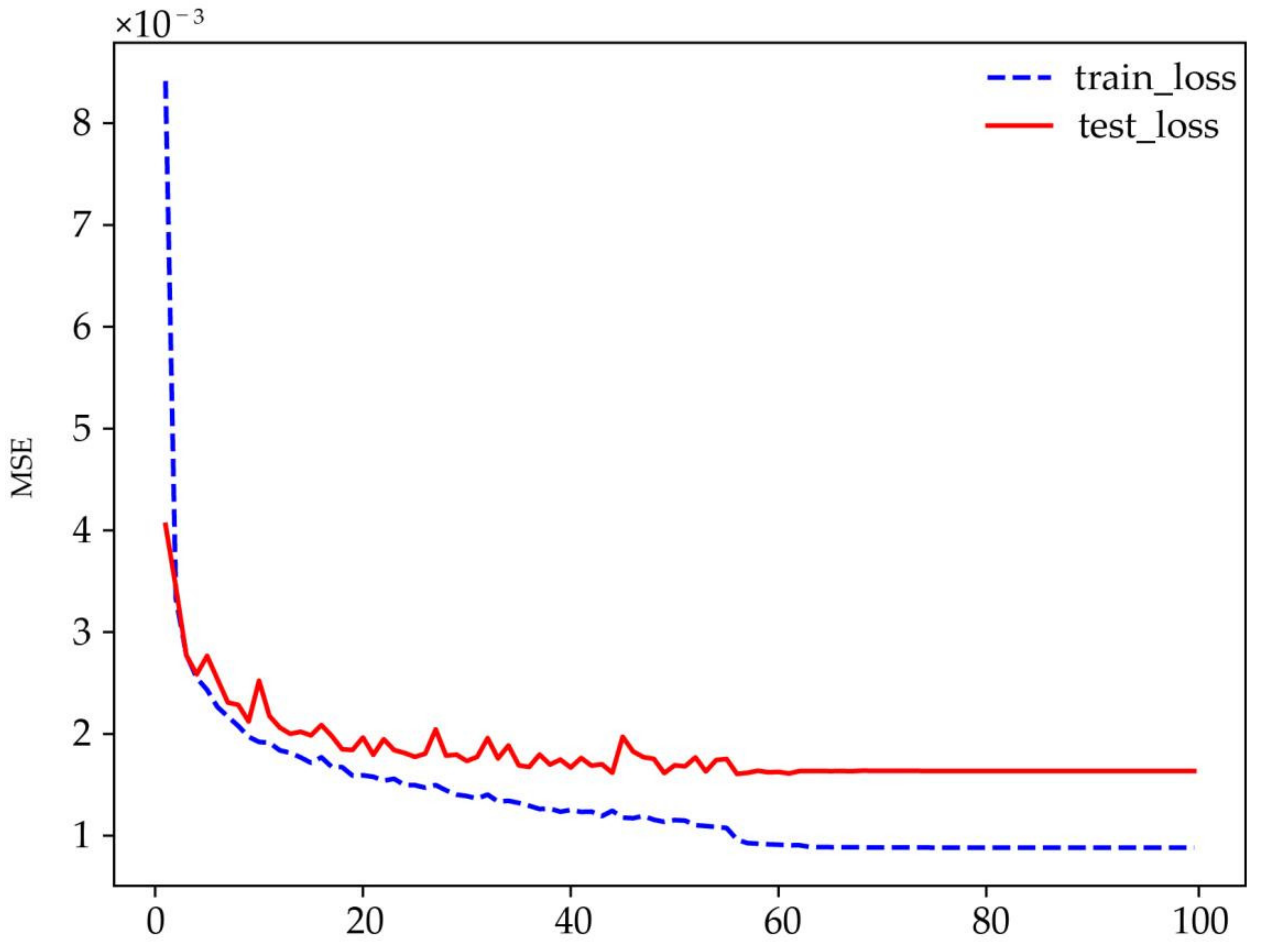
Figure 2 shows the change in loss curves of the training and test dataset, along with the epoch. The values of loss experienced a rapid drop at the beginning of the training and then declined afterward. After the epoch of 60, the loss curve shows the smoothness condition. We saved the parameters according to the performance of the test dataset. Subsequently, we used the trained model to merge the future merged ET data in SSP1–2.6, SSP2–4.5, SSP3–7.0 and SSP5–8.5. For a more intuitive comparison of the DL and traditional MME methods, we re-gridded 22 GCM ET data to 0.25° × 0.25° and merged those GCMs using the MME method.
The four metrics, including MAE, RMSE, ubRMSD and R, were calculated with the test dataset to evaluate the result. Table 2 depicts the difference of those metrics between the DL and MME methods. We can conclude that the DL data show significant improvement in all the metrics. From the MAE, RMSE and ubRMSD, the DL data shows low and abnormal errors in the overall values. The DL data also achieve a high correlation of 0.95. In the following analysis, we compute the spatial MAE of every pixel to understand the spatial error better.
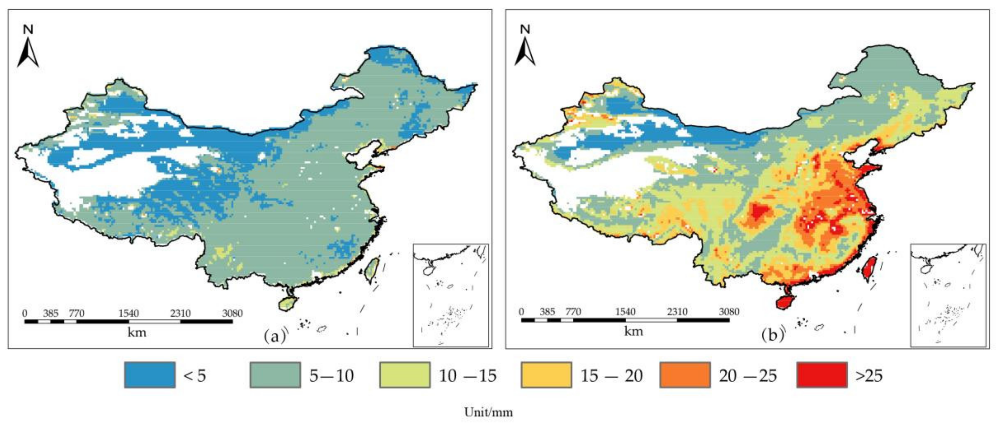
Figure 3 shows the spatial distribution of the MAE. Figure 3a is the MAE of the DL merged data and Figure 3b is the MAE of the MME merged data. From Figure 3a, we can observe that the MAE of most regions is less than 10, while a few regions in the south of China are larger than 10. Compared with the MME result in Figure 3b, the DL merged data greatly improved almost all the pixels. The MME results reflect the raw data error of the GCM data. In eastern China, many regions have an MAE larger than 25. The DL merged data also performed excellently. Figure 3 proved that the DL merged data greatly reduced the loss in the spatial domain. To evaluate DL merged data in the time dimension, we selected four pixels randomly in different climate zones (arid, transition, Tibetan Plateau and humid regions).
The Taylor diagram was used to further evaluate the merged DL, MME, and single GCM data. Figure 4 depicts 25 datasets based on their own distribution of STD, ubRMSD and R. It is obvious that the DL merged data outperforms the other data under all metrics. From the view of R, most of the GCM models range from 0.8 to 0.95. The DL merged data has the best R of 0.95, and the performance of the MME data is second to the DL merged data. Similarly, it can be observed that the DL merged data have the lowest bias and the MME data have less bias than the other GCM models based on the ubRMSD result. The ubRMSD of the majority of the GCM data is around 0.5. From the angle of the STD, it is not surprising that DL merged data is superior to the other data. It is noticeable that the performance of MME data is worse than the GCM data.
The evaluation proves that DL merged data significantly improved in both spatial and temporal dimensions. We used the DL model to merge the future ET data in the SSP1–2.6, SSP2–4.5, SSP3–7.0 and SSP5–8.5. Then, we analyzed the future change in ET in the following work.
3.2. Future Evaporation Change
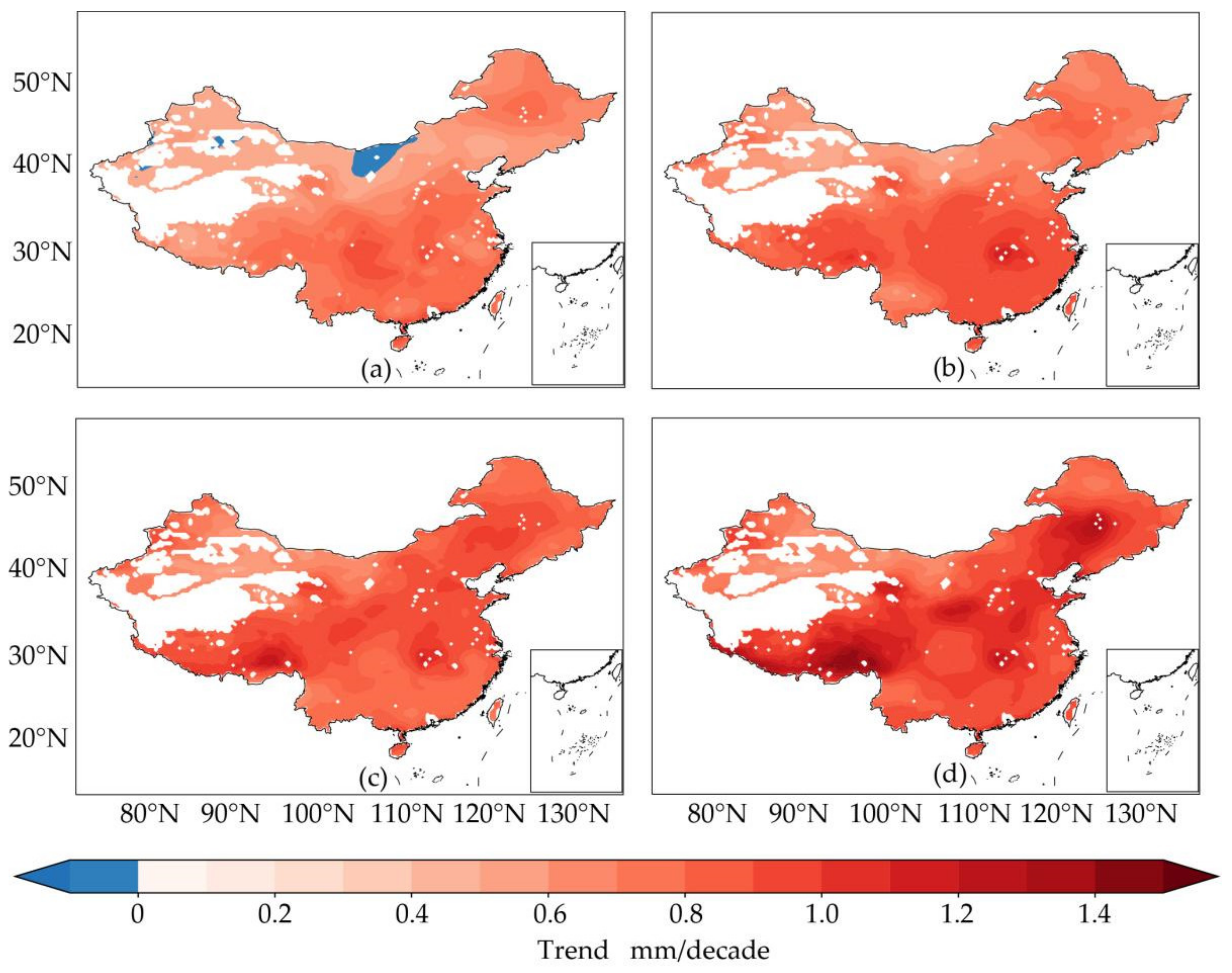
To understand the yearly changes in LET in different scenarios in the future, we calculate the trend of future LET every ten years at every grid and those results are shown the Figure 5. Red indicates the increase in LET, blue indicates the decrease in LET, and the depth of color represents the intensity of the increase and decrease. In general, the trends of LET have some differences in different scenarios. From the low to high scenarios, the increasing trend of LET is more obvious. In the SSP2–4.5, SSP3–7.0 and SSP5–8.5, the LET depicts an upward trend in China, but the intensity of the upward trend was different. The changing trend of LET in SSP1–2.6 was significantly different from that in the other scenarios. In the SSP1–2.6, the overall trend of LET in China is not increasing; there is a downward trend in western Inner Mongolia and a small part of the Xinjiang Province. At the same time, compared with the other three scenarios, the LET trend in China under SSP1–2.6 is not obvious, and the trend of most regions is uniform, about 4mm/decade. In the SSP2–4.5, the trend of LET in southern China is more obvious than in the northern regions. The regions with an obvious upward trend are mainly concentrated in the lower reaches of the Yangtze River Basin and the southern region of the Tibet Plateau, about 8mm/decade. In the SSP3–7.0, the LET in China also shows an upward trend. Compared with the SSP2–4.5, the upward trend is more evident. The regions with the most obvious upward trend are mainly concentrated in the lower reaches of the Yangtze River Basin, the middle reaches of the Yellow River Basin, southern Tibet and southern Northeast China, about 10mm/decade. The LET change trend of SSP5–8.5 is the most significant compared to the other scenarios. The area with a clear LET change trend is relatively consistent with the spatial distribution pattern of the SSP3–7.0, but the trend is more significant.
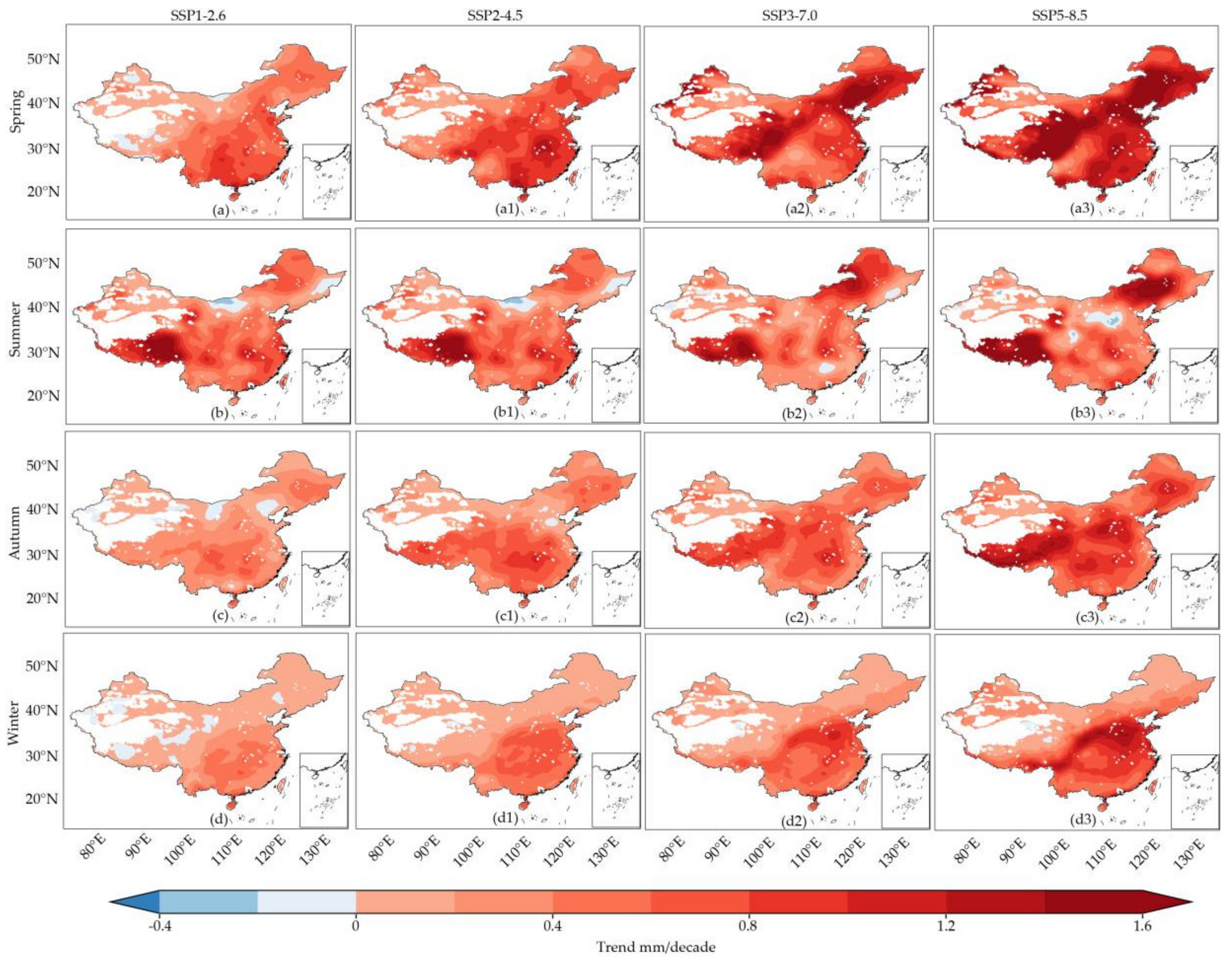
Figure 6 shows the seasonal LET change trend and significant test results in different scenarios. In general, the variation feature of the different seasons is not the same. In the spring, the most obvious increasing regions are in the south of China in the SSP1–2.6, about 0.6 mm/decades. In the northwest of China, some areas demonstrate a downward trend. In the SSP2–4.5, the LET have a similar spatial distribution of the change trend with SSP1–2.6 and the increase in strength is greater than the SSP1–2.6. In addition, the northwest of the China exhibits an upward trend in the SSP2–4.5. In the SSP3–7.0 and SSP5–8.5, almost all the regions that demonstrate an increasing trend and the highest upward areas are the Tibet Plateau and Northeast China. The strength of the upward trend in SSP5–85 is higher than SSP3–7.0 in the Tibet Plateau, about 1.6 mm/decade.
In the summer, the Tibet Plateau shows a higher upward trend than the other regions. In some areas of North China, the downward trend appears in the SSP1–2.6. In the SSP2–4.5, the highest increasing trend is evident in the southeast of China and the Tibet Plateau. The regions in the north of China showed a decreasing trend compared with the SSP1–2.6. In the SSP3–7.0 and SSP5–8.5, the northeast of China and Tibet Plateau reflect the highest upward trend and the upward tendency of SSP5–8.5, which was bigger than the SSP3–7.0.
In the autumn, it is evident that the decreasing trend is lower than the spring and summer trends in all scenarios. In the SSP1–2.6, the trend of most of the increasing regions was less than 0.4mm/decade. The Tibet Plateau and the south of China showed a relatively higher upward tendency than the other regions, about 0.8mm/decade in the SSP2–4.5 and SSP3–7.0. Similarly, the increasing strength was the highest in the SSP5–8.5 compared to the other scenarios. The northeast of China also showed a higher upward trend in SSP5–8.5, in contrast to the Tibet Plateau and the south of China.
In the winter, we can conclude that the upward trend is the lowest out of the four seasons. In the SSP1–2.6, some regions show a decreasing trend in the north of China. Compared to the autumn SSP1–2.6, there is no obvious upward trend in the winter SSP2–4.5. In the other scenarios, the spatial distribution of the trend is similar. The south of China shows a higher upward trend, except for the rise in strength. In the other seasons, the Tibet Plateau demonstrates higher upward trends than the other regions, but the feature is not found in the winter.
4. Discussion
4.1. Data Merge and Downscaling of Climate Data
In this work, we innovatively applied a DL-based method to carry out the data merge and downscaling of GCM data. The input data of the DL model was 22 GCM, with the spatial resolution at 2° × 2° and the output of the DL model was one set of merged higher resolution data at 0.25° × 0.25°. The merged data greatly improved the correlation and bias from all the evaluation metrics. In the previous work, the successful application of the DL model from the SR field regarding soil moisture and air temperature was reported [48]. Our work also proves the DL model can carry out the data merge and data downscaling simultaneously. The DL methods can make full use of the information of each GCM and merge more accurate data.
4.2. Future Spatial-Temporal Changes in LET
Previous research reports that the increasing global trend of LET is consistent with the trend in China [49,50]. In the other regions of the world, the LET reflects a different trend, such as a decrease in South America and an increase in North America and Greece [51,52,53]. Thus, it is important to understand the LET changes in the regional areas [54]. According to our result, the future changes in LET are evidenced by the increasing trend in China, from the low scenario to high scenario; the intensity of the upward trend is increasing. This result is similar with the related research in China [3,55]. In general, the highest upward trend can be found in the Tibet Plateau, followed by the south of China in the humid regions. From a seasonal view, the increasing trend in the spring and summer is far larger than in autumn and winter. The same conclusion can be drawn that the highest upward regions include the Tibet Plateau and the humid region in the south of China.
4.3. Limitation and Prospect
Our work includes some limitations. First, because there is not enough weather observation data, the reference LET data of this work include merged data based on remote sensing data and reanalysis data. These data have certain errors themselves. In the next work, we need take more observation data as the reference data. Secondly, the DL model we used in our work did not consider time information and the climate data had redundant time information. In the next work, we can use the DL models that consider the time dimension [56].
5. Conclusions
This work applied a DL model named Ynet to form a high-resolution dataset based on the GCMs in China. The methods mentioned in this paper can carry out data downscaling and date merging simultaneously. We used the DL model to learn about the relationship between the reference data and GCMs in the specified time period. Then, we applied the trained model to merge the GCMs in the future scenarios (SSP1–2.6, SSP2–4.5, SSP3–7.0 and SSP5–8.5). The results in the test dataset demonstrate that the DL merged data significantly improve the GCM data in all aspects, according to different evaluation metrics. Most regions of China show a low error level.
We analyzed the future spatial-temporal changes in different scenarios using the DL merged data. Generally, from low to high, the intensity of the upward trend rises in China. From the yearly change scale, in the SSP1–2.6 and SSP2–4.5, we can observe the highest increasing regions compared to the other areas. In the SSP3–7.0 and SSP5–8.5, the Tibet Plateau has the tallest upward trend compared to the other places, with about 10mm/decade in SSP3–7.0 and 14 mm/decade in SSP5–8.5. In addition, the increasing trend of the humid regions in the south of China is ranked second to the Tibet Plateau in those two high scenarios. The seasonal changes show the highest increasing trend in spring. The increasing intensity decreases from the spring to winter. The Tibet Plateau and the northeast of China demonstrate the largest upward trends in the spring of SSP5–8.5, which is higher than 1.6 mm/decade.
Author Contributions
Conceptualization, X.N. and G.W.; methodology, X.W.; software, X.W.; investigation, X.N. and W.Z.; data curation, W.T.; writing—original draft preparation, X.N.; writing—review and editing, X.N.; supervision, X.N.; funding, G.W. All authors have read and agreed to the published version of the manuscript.
Funding
This work is funded by the 173 National Basic Research Program of China (2020-JCJQ-ZD-087-01).
Data Availability Statement
The data used in this study can be downloaded from https://doi.org/10.5281/zenodo.4595941 and https://esgf-node.llnl.gov/projects/cmip6/.
Conflicts of Interest
The authors declare no conflict of interest.
References
- Ma, J.; Chadwick, R.; Seo, K.H.; Dong, C.; Huang, G.; Foltz, G.R.; Jiang, J.H. Responses of the tropical atmospheric circulation to climate change and connection to the hydrological cycle. Annu. Rev. Earth Planet. Sci. 2018, 46, 549–580. [Google Scholar] [CrossRef]
- Zohaib, M.; Kim, H.; Choi, M. Evaluating the patterns of spatiotemporal trends of root zone soil moisture in major climate regions in East Asia. J. Geophys. Res. Atmos. 2017, 122, 7705–7722. [Google Scholar] [CrossRef]
- Lu, J.; Wang, G.; Li, S.; Feng, A.; Zhan, M.; Jiang, T.; Su, B.; Wang, Y. Projected Land Evaporation and Its Response to Vegetation Greening over China Under Multiple Scenarios in the CMIP6 Models. J. Geophys. Res. Biogeosci. 2021, 126, e2021JG006327. [Google Scholar] [CrossRef]
- Lu, J.; Sun, G.; McNulty, S.G.; Amatya, D.M. Modeling actual evapotranspiration from forested watersheds across the southeastern united states. JAWRA J. Am. Water Resour. Assoc. 2003, 39, 886–896. [Google Scholar] [CrossRef]
- Jun, W.; Xinhua, W.; Meihua, G.; Xuyan, X. Impact of Climate Change on Reference Crop Evapotranspiration in Chuxiong City, Yunnan Province. Procedia Earth Planet. Sci. 2012, 5, 113–119. [Google Scholar] [CrossRef]
- Montroull, N.B.; Saurral, R.I.; Camilloni, I.A. Hydrological impacts in La Plata basin under 1.5, 2 and 3 °C global warming above the pre-industrial level. Int. J. Clim. 2018, 38, 3355–3368. [Google Scholar] [CrossRef]
- Eyring, V.; Cox, P.M.; Flato, G.M.; Gleckler, P.J.; Abramowitz, G.; Caldwell, P.; Collins, W.D.; Gier, B.K.; Hall, A.D.; Hoffman, F.M.; et al. Taking climate model evaluation to the next level. Nat. Clim. Chang. 2019, 9, 102–110. [Google Scholar] [CrossRef]
- Van Vuuren, D.P.; Kriegler, E.; O’Neill, B.C.; Ebi, K.L.; Riahi, K.; Carter, T.R.; Edmonds, J.; Hallegatte, S.; Kram, T.; Mathur, R.; et al. A new scenario framework for Climate Change Research: Scenario matrix architecture. Clim. Chang. 2013, 122, 373–386. [Google Scholar] [CrossRef]
- Riahi, K.; Van Vuuren, D.P.; Kriegler, E.; Edmonds, J.; O’Neill, B.C.; Fujimori, S.; Bauer, N.; Calvin, K.; Dellink, R.; Fricko, O.; et al. The Shared Socioeconomic Pathways and their energy, land use, and greenhouse gas emissions implications: An overview. Glob. Environ. Chang. 2016, 42, 153–168. [Google Scholar] [CrossRef]
- Fricko, O.; Havlik, P.; Rogelj, J.; Klimont, Z.; Gusti, M.; Johnson, N.; Kolp, P.; Strubegger, M.; Valin, H.; Amann, M. The marker quantification of the Shared Socioeconomic Pathway 2: A middle-of-the-road scenario for the 21st century. Glob. Environ. Chang. 2017, 42, 251–267. [Google Scholar] [CrossRef] [Green Version]
- Fujimori, S.; Hasegawa, T.; Masui, T.; Takahashi, K.; Herran, D.S.; Dai, H.; Hijioka, Y.; Kainuma, M. SSP3: AIM implementation of Shared Socioeconomic Pathways. Glob. Environ. Chang. 2017, 42, 268–283. [Google Scholar] [CrossRef]
- Calvin, K.; Bond-Lamberty, B.; Clarke, L.; Edmonds, J.; Eom, J.; Hartin, C.; Kim, S.; Kyle, P.; Link, R.; Moss, R.; et al. The SSP4: A world of deepening inequality. Glob. Environ. Chang. 2017, 42, 284–296. [Google Scholar] [CrossRef]
- Kriegler, E.; Bauer, N.; Popp, A.; Humpenöder, F.; Leimbach, M.; Strefler, J.; Baumstark, L.; Bodirsky, B.L.; Hilaire, J.; Klein, D.; et al. Fossil-fueled development (SSP5): An energy and resource intensive scenario for the 21st century. Glob. Environ. Chang. 2017, 42, 297–315. [Google Scholar] [CrossRef]
- Turner, D.P.; Conklin, D.R.; Vache, K.B.; Schwartz, C.; Nolin, A.W.; Chang, H.; Watson, E.; Bolte, J.P. Assessing mechanisms of climate change impact on the upland forest water balance of the Willamette River Basin, Oregon. Ecohydrology 2017, 10, e1776. [Google Scholar] [CrossRef]
- Parsons, L.A.; Brennan, M.K.; Wills, R.C.; Proistosescu, C. Magnitudes and Spatial Patterns of Interdecadal Temperature Variability in CMIP6. Geophys. Res. Lett. 2020, 47, e2019GL086588. [Google Scholar] [CrossRef]
- Li, B.; Rodell, M.; Zaitchik, B.F.; Reichle, R.H.; Koster, R.D.; van Dam, T.M. Assimilation of GRACE terrestrial water storage into a land surface model: Evaluation and potential value for drought monitoring in western and central Europe. J. Hydrol. 2012, 446–447, 103–115. [Google Scholar] [CrossRef]
- Deser, C.; Phillips, A.; Bourdette, V.; Teng, H. Uncertainty in climate change projections: The role of internal variability. Clim. Dyn. 2012, 38, 527–546. [Google Scholar] [CrossRef]
- Zhuan, M.; Chen, J.; Xu, C.-Y.; Zhao, C.; Xiong, L.; Liu, P. A method for investigating the relative importance of three components in overall uncertainty of climate projections. Int. J. Clim. 2018, 39, 1853–1871. [Google Scholar] [CrossRef]
- Zhang, S.; Chen, J. Uncertainty in Projection of Climate Extremes: A Comparison of CMIP5 and CMIP6. J. Meteorol. Res. 2021, 35, 646–662. [Google Scholar] [CrossRef]
- Weigel, A.P.; Liniger, M.A.; Appenzeller, C. Can multi-model combination really enhance the prediction skill of probabilistic ensemble forecasts? Q. J. R. Meteorol. Soc. 2008, 134, 241–260. [Google Scholar] [CrossRef]
- White, R.H.; Toumi, R. The limitations of bias correcting regional climate model inputs. Geophys. Res. Lett. 2013, 40, 2907–2912. [Google Scholar] [CrossRef]
- Maraun, D.; Widmann, M. Structure of statistical downscaling methods. In Statistical Downscaling and Bias Correction for Climate Research; Cambridge University Press: Cambridge, UK, 2018; pp. 135–140. [Google Scholar]
- Adachi, S.A.; Tomita, H. Methodology of the constraint condition in dynamical downscaling for regional climate evaluation: A review. J. Geophys. Res. Atmos. 2020, 125, e2019JD032166. [Google Scholar] [CrossRef]
- Zhu, J.; Huang, G.; Wang, X.; Cheng, G.; Wu, Y. High-resolution projections of mean and extreme precipitations over China through PRECIS under RCPs. Clim. Dyn. 2018, 50, 4037–4060. [Google Scholar] [CrossRef]
- Stefanidis, S. Ability of Different Spatial Resolution Regional Climate Model to Simulate Air Temperature in a Forest Ecosystem of Central Greece. J. Environ. Prot. Ecol. 2021, 22, 1488–1495. [Google Scholar]
- Xue, Y.; Janjic, Z.; Dudhia, J.; Vasic, R.; De Sales, F. A review on regional dynamical downscaling in intraseasonal to seasonal simulation/prediction and major factors that affect downscaling ability. Atmospheric Res. 2014, 147–148, 68–85. [Google Scholar] [CrossRef]
- Sachindra, D.; Ahmed, K.; Rashid, M.; Shahid, S.; Perera, B. Statistical downscaling of precipitation using machine learning techniques. Atmos. Res. 2018, 212, 240–258. [Google Scholar] [CrossRef]
- Das, L.; Akhter, J. How well are the downscaled CMIP5 models able to reproduce the monsoon precipitation over seven homogeneous zones of India? Int. J. Clim. 2019, 39, 3323–3333. [Google Scholar] [CrossRef]
- Asong, Z.; Khaliq, M.; Wheater, H. Projected changes in precipitation and temperature over the Canadian Prairie Provinces using the Generalized Linear Model statistical downscaling approach. J. Hydrol. 2016, 539, 429–446. [Google Scholar] [CrossRef]
- Miao, C.; Ashouri, H.; Hsu, K.-L.; Sorooshian, S.; Duan, Q. Evaluation of the PERSIANN-CDR Daily Rainfall Estimates in Capturing the Behavior of Extreme Precipitation Events over China. J. Hydrometeorol. 2015, 16, 1387–1396. [Google Scholar] [CrossRef]
- Ho, C.K.; Stephenson, D.B.; Collins, M.; Ferro, C.A.T.; Brown, S.J. Calibration Strategies: A Source of Additional Uncertainty in Climate Change Projections. Bull. Am. Meteorol. Soc. 2012, 93, 21–26. [Google Scholar] [CrossRef]
- Fang, G.H.; Yang, J.; Chen, Y.N.; Zammit, C. Comparing bias correction methods in downscaling meteorological variables for a hydrologic impact study in an arid area in China. Hydrol. Earth Syst. Sci. 2015, 19, 2547–2559. [Google Scholar] [CrossRef] [Green Version]
- Themeßl, M.J.; Gobiet, A.; Leuprecht, A. Empirical-statistical downscaling and error correction of daily precipitation from regional climate models. Int. J. Climatol. 2011, 31, 1530–1544. [Google Scholar] [CrossRef]
- Bruyère, C.L.; Done, J.M.; Holland, G.J.; Fredrick, S. Bias corrections of global models for regional climate simulations of high-impact weather. Clim. Dyn. 2014, 43, 1847–1856. [Google Scholar] [CrossRef]
- Colette, A.; Vautard, R.; Vrac, M. Regional climate downscaling with prior statistical correction of the global climate forcing. Geophys. Res. Lett. 2012, 39, L13707. [Google Scholar] [CrossRef]
- Reichstein, M.; Camps-Valls, G.; Stevens, B.; Jung, M.; Denzler, J.; Carvalhais, N.; Prabhat. Deep learning and process understanding for data-driven Earth system science. Nature 2019, 566, 195–204. [Google Scholar] [CrossRef]
- Ham, Y.-G.; Kim, J.-H.; Luo, J.-J. Deep learning for multi-year ENSO forecasts. Nature 2019, 573, 568–572. [Google Scholar] [CrossRef]
- Kadow, C.; Hall, D.M.; Ulbrich, U. Artificial intelligence reconstructs missing climate information. Nat. Geosci. 2020, 13, 408–413. [Google Scholar] [CrossRef]
- Tian, L.; Sun, J.; Chang, J.; Xia, J.; Zhang, Z.; Kolomenskii, A.A.; Schuessler, H.A.; Zhang, S. Retrieval of gas concentrations in optical spectroscopy with deep learning. Measurement 2021, 182, 109739. [Google Scholar] [CrossRef]
- Yoon, Y.; Jeon, H.-G.; Yoo, D.; Lee, J.-Y.; Kweon, I.S. Learning a Deep Convolutional Network for Light-Field Image Super-Resolution. In Proceedings of the 2015 IEEE International Conference on Computer Vision Workshop (ICCVW), Santiago, Chile, 7–13 December 2015; pp. 57–65. [Google Scholar] [CrossRef]
- Zhang, L.; Nie, J.; Wei, W.; Zhang, Y.; Liao, S.; Shao, L. Unsupervised Adaptation Learning for Hyperspectral Imagery Super-Resolution. In Proceedings of the 2020 IEEE/CVF Conference on Computer Vision and Pattern Recognition (CVPR), Seattle, WA, USA, 13–19 June 2020; pp. 3070–3079. [Google Scholar] [CrossRef]
- Chen, Y.; Liu, S.; Wang, X. Learning continuous image representation with local implicit image function. In Proceedings of the IEEE/CVF Conference on Computer Vision and Pattern Recognition, Nashville, TN, USA, 20–25 June 2021; pp. 8628–8638. [Google Scholar]
- Vandal, T.; Kodra, E.; Ganguly, S.; Michaelis, A.; Nemani, R.; Ganguly, A. Generating High Resolution Climate Change Projections through Single Image Super-Resolution. In Proceedings of the 23rd ACM SIGKDD International Conference on Knowledge Discovery and Data Mining (KDD ‘17), Halifax, NS, Canada, 13–17 August 2017; Association for Computing Machinery: New York, NY, USA, 2017; pp. 1663–1672. [Google Scholar]
- Rodrigues, E.R.; Oliveira, I.; Cunha, R.; Netto, M. DeepDownscale: A deep learning strategy for high-resolution weather forecast. In Proceedings of the 2018 IEEE 14th International Conference on e-Science (e-Science), Amsterdam, The Netherlands, 29 October–1 November 2018; IEEE: Piscataway, NJ, USA, 2018; pp. 415–422. [Google Scholar]
- Lu, J.; Wang, G.; Chen, T.; Li, S.; Hagan, D.F.T.; Kattel, G.; Peng, J.; Jiang, T.; Su, B. A harmonized global land evaporation dataset from model-based products covering 1980–2017. Earth Syst. Sci. Data 2021, 13, 5879–5898. [Google Scholar] [CrossRef]
- Liu, Y.; Ganguly, A.R.; Dy, J. Climate Downscaling Using YNet. In Proceedins of the 26th ACM SIGKDD International Conference on Knowledge Discovery and Data Mining, Virtual Event, CA, USA, 6–10 July 2020; pp. 3145–3153. [Google Scholar] [CrossRef]
- Taylor, K.E. Summarizing multiple aspects of model performance in a single diagram. J. Geophys. Res. Atmos. 2001, 106, 7183–7192. [Google Scholar] [CrossRef]
- Feng, D.; Wang, G.; Wei, X.; Amankwah, S.O.Y.; Hu, Y.; Luo, Z.; Hagan, D.F.T.; Ullah, W. Merging and Downscaling Soil Moisture Data From CMIP6 Projections Using Deep Learning Method. Front. Environ. Sci. 2022, 10. [Google Scholar] [CrossRef]
- Wang, Z.; Zhan, C.; Ning, L.; Guo, H. Evaluation of global terrestrial evapotranspiration in CMIP6 models. Arch. Meteorol. Geophys. Bioclimatol. Ser. B 2021, 143, 521–531. [Google Scholar] [CrossRef]
- Niu, Z.; Wang, L.; Chen, X.; Yang, L.; Feng, L. Spatiotemporal distributions of pan evaporation and the influencing factors in China from 1961 to 2017. Environ. Sci. Pollut. Res. 2021, 28, 68379–68397. [Google Scholar] [CrossRef] [PubMed]
- Brêda, J.P.; de Paiva, R.C.; Collischon, W.; Bravo, J.M.; Siqueira, V.A.; Steinke, E.B. Climate change impacts on South American water balance from a continental-scale hydrological model driven by CMIP5 projections. Clim. Chang. 2020, 159, 503–522. [Google Scholar] [CrossRef]
- Sullivan, R.C.; Kotamarthi, V.R.; Feng, Y. Recovering Evapotranspiration Trends from Biased CMIP5 Simulations and Sensitivity to Changing Climate over North America. J. Hydrometeorol. 2019, 20, 1619–1633. [Google Scholar] [CrossRef]
- Stefanidis, S.; Alexandridis, V. Precipitation and Potential Evapotranspiration Temporal Variability and Their Relationship in Two Forest Ecosystems in Greece. Hydrology 2021, 8, 160. [Google Scholar] [CrossRef]
- Ajjur, S.B.; Al-Ghamdi, S.G. Evapotranspiration and water availability response to climate change in the Middle East and North Africa. Clim. Chang. 2021, 166, 28. [Google Scholar] [CrossRef]
- Zhan, M.Y.; Wang, G.J.; Lu, J.; Chen, L.Q.; Zhu, C.X.; Jiang, T.; Wang, Y.J. Projected evapotranspiration and the influencing factors in the Yangtze River Basin based on CMIP6 models. Trans. Atmos. Sci. 2020, 43, 1115–1126. (In Chinese) [Google Scholar] [CrossRef]
- Wang, X.; Chan, K.C.; Yu, K.; Dong, C.; Loy, C.C. EDVR: Video Restoration with Enhanced Deformable Convolutional Networks. In Proceedings of the 2019 IEEE/CVF Conference on Computer Vision and Pattern Recognition Workshops (CVPRW), Long Beach, CA, USA, 16–17 June 2019; pp. 1954–1963. [Google Scholar] [CrossRef] [Green Version]
Figure 1.
The location of the study area.

Figure 2.
The loss value of training and test dataset per epoch.

Figure 3.
The spatial MAE distribution of the DL and MME methods in the test dataset, (a) DL merged data, (b) MME merged data.
Figure 3.
The spatial MAE distribution of the DL and MME methods in the test dataset, (a) DL merged data, (b) MME merged data.

Figure 4.
The Taylor diagram of the monthly DL merged data, MME data and single GCM data in the period of the test dataset (2008–2014). The Y axis shows the standard deviation (STD), ubRMSD is depicted by the green circles with dashed lines and the angular coordinate is applied to represent R.
Figure 4.
The Taylor diagram of the monthly DL merged data, MME data and single GCM data in the period of the test dataset (2008–2014). The Y axis shows the standard deviation (STD), ubRMSD is depicted by the green circles with dashed lines and the angular coordinate is applied to represent R.

Figure 5.
The yearly trend of future evaporation change from 2021–2100 in different scenarios. (a–d) correspond to the SSP1–2.6, SSP2–4.5, SSP3–7.0 and SSP5–8.5 scenarios, respectively.
Figure 5.
The yearly trend of future evaporation change from 2021–2100 in different scenarios. (a–d) correspond to the SSP1–2.6, SSP2–4.5, SSP3–7.0 and SSP5–8.5 scenarios, respectively.

Figure 6.
The seasonal trend of future LET change from 2021 to 2100 in different scenarios; (a–d) correspond to spring, summer, autumn and winter, respectively. The (a), (a1), (a2) and (a3) correspond to the future spring change in SSP1–2.6, SSP2–4.5, SSP3–7.0 and SSP5–8.5. The (b), (b1), (b2) and (b3) correspond to the future summer change in SSP1–2.6, SSP2–4.5, SSP3–7.0 and SSP5–8.5. The (c), (c1), (c2) and (c3) correspond to the future autumn change in SSP1–2.6, SSP2–4.5, SSP3–7.0 and SSP5–8.5. The (d), (d1), (d2) and (d3) correspond to the future winter change in SSP1–2.6, SSP2–4.5, SSP3–7.0 and SSP5–8.5.


Table 1.
GCM and their grid size resolutions used in the current study.
| Institution (Country) | Model Name | Resolution (Lon × Lat) | Used Member |
|---|---|---|---|
| CSIRO (Australia) | ACCESS-CM2 | 1.875° × 1.25° | r1i1p1f1 |
| BCC (China) | BCC-CSM2-MR | 2.25° × 2.25° | r1i1p1f1 |
| CAMS (China) | CAMS-CSM1-0 | 1.125° × 1.125° | r1i1p1f1 |
| NCAR (USA) | CESM2-WACCM | 2.5° × 1.875° | r1i1p1f1 |
| CESM2 | r1i1p1f1 | ||
| CNRM-CERFACS (France) | CNRM-CM6-1-HR | 1.25° × 0.9375° | r1i1p1f2 |
| CNRM-ESM2-1 | r1i1p1f2 | ||
| CCCMA (Canada) | CanESM5 | 2.8125° × 2.8125° | r1i1p1f1 |
| EC-Earth Consortium (EU) | EC-Earth3-Veg | 0.703125° × 0.703125° | r1i1p1f1 |
| CAS (China) | FGOALS-f3-L | 2.5° × 2° | r1i1p1f1 |
| NOAA-GFDL (USA) | GFDL-ESM4 | 2.5° × 2° | r1i1p1f1 |
| INM (Russia) | INM-CM4-8 | 2° × 1.5° | r1i1p1f1 |
| INM-CM5-0 | r1i1p1f1 | ||
| IPSL (France) | IPSL-CM6A-LR | 2.5° × 1.259° | r1i1p1f1 |
| MIROC (Japan) | MIROC-ES2L | 2.8125° × 2.8125° | r1i1p1f2 |
| MIROC6 | 2.8125° × 0.703125° | r1i1p1f1 | |
| MPI-M (Germany) | MPI-ESM1-2-HR | 0.9375° × 0.9375° | r1i1p1f1 |
| MPI-ESM1-2-LR | 1.875° × 1.875° | r1i1p1f1 | |
| MRI (Japan) | MRI-ESM2-0 | 1.125° × 1.125° | r1i1p1f1 |
| NCC (Norway) | NorESM2-LM | 5° × 3.75° | r1i1p1f1 |
| NorESM2-MM | 2.5° × 1.875° | r1i1p1f1 | |
| MOHC (UK) | UKESM1-0-LL | 1.875° × 1.25° | r1i1p1f2 |
Table 2.
Different evaluation metrics in test dataset of DL and MEM methods.
| Methods | MAE | RMSE | ubRMSD | R |
|---|---|---|---|---|
| DL data | 5.91 | 5.86 | 5.88 | 0.95 |
| MEM data | 14.63 | 21.16 | 19.01 | 0.85 |
Publisher’s Note: MDPI stays neutral with regard to jurisdictional claims in published maps and institutional affiliations. |
© 2022 by the authors. Licensee MDPI, Basel, Switzerland. This article is an open access article distributed under the terms and conditions of the Creative Commons Attribution (CC BY) license (https://creativecommons.org/licenses/by/4.0/).
Share and Cite
MDPI and ACS Style
Niu, X.; Wei, X.; Tian, W.; Wang, G.; Zhu, W. The Future Change in Evaporation Based on the CMIP6 Merged Data Generated by Deep-Learning Method in China. Water 2022, 14, 2800. https://doi.org/10.3390/w14182800
AMA Style
Niu X, Wei X, Tian W, Wang G, Zhu W. The Future Change in Evaporation Based on the CMIP6 Merged Data Generated by Deep-Learning Method in China. Water. 2022; 14(18):2800. https://doi.org/10.3390/w14182800
Chicago/Turabian StyleNiu, Xianghua, Xikun Wei, Wei Tian, Guojie Wang, and Wenhui Zhu. 2022. "The Future Change in Evaporation Based on the CMIP6 Merged Data Generated by Deep-Learning Method in China" Water 14, no. 18: 2800. https://doi.org/10.3390/w14182800
Note that from the first issue of 2016, this journal uses article numbers instead of page numbers. See further details here.