Modelling Soil Water, Salt and Heat Dynamics under Partially Mulched Conditions with Drip Irrigation, Using HYDRUS-2D

Abstract

Drip irrigation under mulch is a widely used technique in the arid region of northwest China. The partially mulched soil and the bare strips between mulched areas may complicate the migration of water, salt, and heat in soils, and cause lateral salt accumulation on bare soil surfaces. For investigating hydrothermal dynamics and salt distribution patterns under such circumstances, tank experiments with drip irrigation under plastic film on partially mulched soil were conducted under two intensities of drip irrigation (i.e., low (W1) and high (W2)) with the same total irrigation amount. The spatial distributions of soil water, temperature, and electrical conductivity were monitored accordingly. The two-dimensional (2D) model of soil water, salt, and heat transport under drip irrigation and partially mulched soil conditions was established using HYDRUS-2D, and kinetic adsorption during salt migration was considered. The results of the experiments showed that the uneven distribution of the hydrothermal state led to the accumulation of salt on the un-mulched soil surface. Water migrated from where the dripper was located, and heat accumulated mainly in the mulched soil. HYDRUS-2D matched reasonably well with the observed data, with an ${\mathrm{R}}^2$ higher than 0.54. Under the partially mulched conditions, lower intensity of drip irrigation (W1) show higher desalination efficiency in root zones, with less even lateral salt distribution. Scenario simulations further demonstrated that a larger total irrigation amount would result in a larger desalination zone, and drip irrigations with appropriate incremental intensity could improve salt leaching in the root zone with increased lateral migration of water.

1. Introduction

Soil salinity and water shortages are two major threats to world food security; 33% of irrigation agricultural lands have severely suffered from soil salinization, and more than 60% of farmland is limited by water shortages [1]. Northwest China, a significant food-producing area, is a typical arid region that is rich in light, heat, and land resources. Water shortage and soil salinization are two major problems restricting the sustainable development of agriculture in this area [2,3]. Furthermore, high potential evaporation exacerbates the soil salinity problem [4]. Film mulching can effectively reduce soil evaporation by hindering water exchange between the soil and the outside environment [5,6,7]. In addition, drip irrigation is commonly used as a water-saving measure, and significantly improves water productivity and crop yields compared with conditional flood irrigation [8,9,10]. Combining the above advantages, one can see that drip irrigation under mulch conditions can conserve water and heat, which is beneficial for crop growth and crop yield [11,12]. This technology has been widely applied in northwest China; the application area occupies more than 1.6 million ${\mathrm{hm}}^2$ in Xinjiang, and continues to increase [13,14].

Despite the above advantages, water-saving irrigation such as drip irrigation may not effectively leach salt out of the root zone, thus potentially causing salt accumulation and harming crop growth [13,15]. Film mulching can inhibit soil evaporation and salinization to a certain extent, especially in combination with drip irrigation [16]. However, where bare strips exist between mulched soil, uneven distribution of water and heat appears, leading to salt accumulation in these places. This complex salt distribution pattern has the potential to cause salinization problems in the long term. For scientific water and salt transport on farmland, it is crucial to understand the mechanisms of water, salt, and heat migration with drip irrigation under partially mulched soil conditions.

In recent years, many researchers have investigated water, salt, and heat transport in bare soil under drip irrigation conditions, through lab and field experiments combined with numerical simulations. In bare farmland soil, drip irrigation has usually been regarded as a line source; thus, HYDRUS-2D can be used to investigate water, salt, and heat transport in the vertical soil profile. For example, Wang et al. [17] used HYDRUS-2D to simulate and verify water flow and heat transport around the subsurface drip line. Selim et al. [18] employed HYDRUS-2D to simulate water and salt distribution for surface drip irrigation with brackish irrigation water under various scenarios of soil quality, initial water content, and irrigation frequency. In addition, with the dripper regarded as a point source, Antonio et al. [19] used HYDRUS-3D to study water migration behavior in layered soil. Shan et al. [20] investigated the watersalt transport in the intersection area between two point sources. These previous results, based on simulations by HYDRUS-2D/3D, discussed the laws of water, salt, and heat transport in bare farmland soil and determined ideal irrigation practices. Under totally mulched soil conditions, Zhao et al. [21] simulated one-dimensional (1D) soil, water, and heat transport in the vertical direction under different irrigation quantities. In addition, Qi et al. [22] found that full film mulching contributed to an obvious desalination effect on soil under drip irrigation.

For typical drip irrigation under partially mulched conditions, the bare strips between mulched soil can cause large heterogeneity in water, salt, and heat distribution within the soil surface [23,24,25]. Experiments showed that irrigation [26], salinity [27,28], and tillage management [22] could affect soil moisture, salinity, and heat dynamics in mulched and un-mulched strips. Some studies combined field and indoor soil tank experiments to explore water and salt distribution influenced by agriculture methods, e.g., horizontal tillage or salt drainage ditches [29,30]. Meanwhile, HYDRUS-2D was successfully applied to describe the mechanism of soil water, salt, and heat transport with lateral differences [31,32]. Combining HYDRUS-2D with field experiments, Qi et al. [22] investigated spatial soil moisture and salt distribution under partially mulched drip irrigation, and found that it led to secondary salinization in a 0 to 40 cm layer in the un-mulched soil under flat tillage. In addition, the flow rate, total quantity, and frequency also affected such spatial differences [26,33]. Ning et al. [28] used HYDRUS-2D combined with field experiments to investigate salt storage in the root zone, and they found that a high irrigation amount with low drip irrigation frequency promoted soil desalination.

Despite these various advancements, most articles related to partially mulched drip irrigation have focused either on field experiments, which involve high levels of spatial heterogeneity in soil and are less controllable, or indoor experiments targeting the influence of specific agriculture measures. These previous studies have lacked in-depth analysis of the mechanism of salt migration. In addition, in previous simulations, salt has generally been regarded as conservative particle, while in reality, salt transport is accompanied by physical and chemical reactions (e.g., adsorption–desorption, precipitation–dissolution, etc.). Evaporation was found to be accompanied by latent heat consumption, and soil surface temperatured varied under partially mulched conditions, indicating that heat transport cannot be neglected in the investigation of water and salt transport. Hence, for thoroughly investigating salt behavior under partially mulched drip irrigation, it is necessary to construct a 2D model of water, salt, and heat transport that includes bare and mulched soil areas, and involves the typical salt reactions. To this end, the main goal of this study was to investigate water, salt, and heat dynamics of soil under partially mulched drip irrigation, combining laboratory experiments and HYDRUS-2D model software. The model distinguished mulched and un-mulched areas, and considered the kinetic adsorption process in salt migration. Finally, the influence of various drip-irrigation intensities on the spatial distribution of soil water, salt, and temperature was analyzed, as was salt leaching efficiency under various drip irrigation conditions.

2. Materials and Methods

2.1. Experimental Design

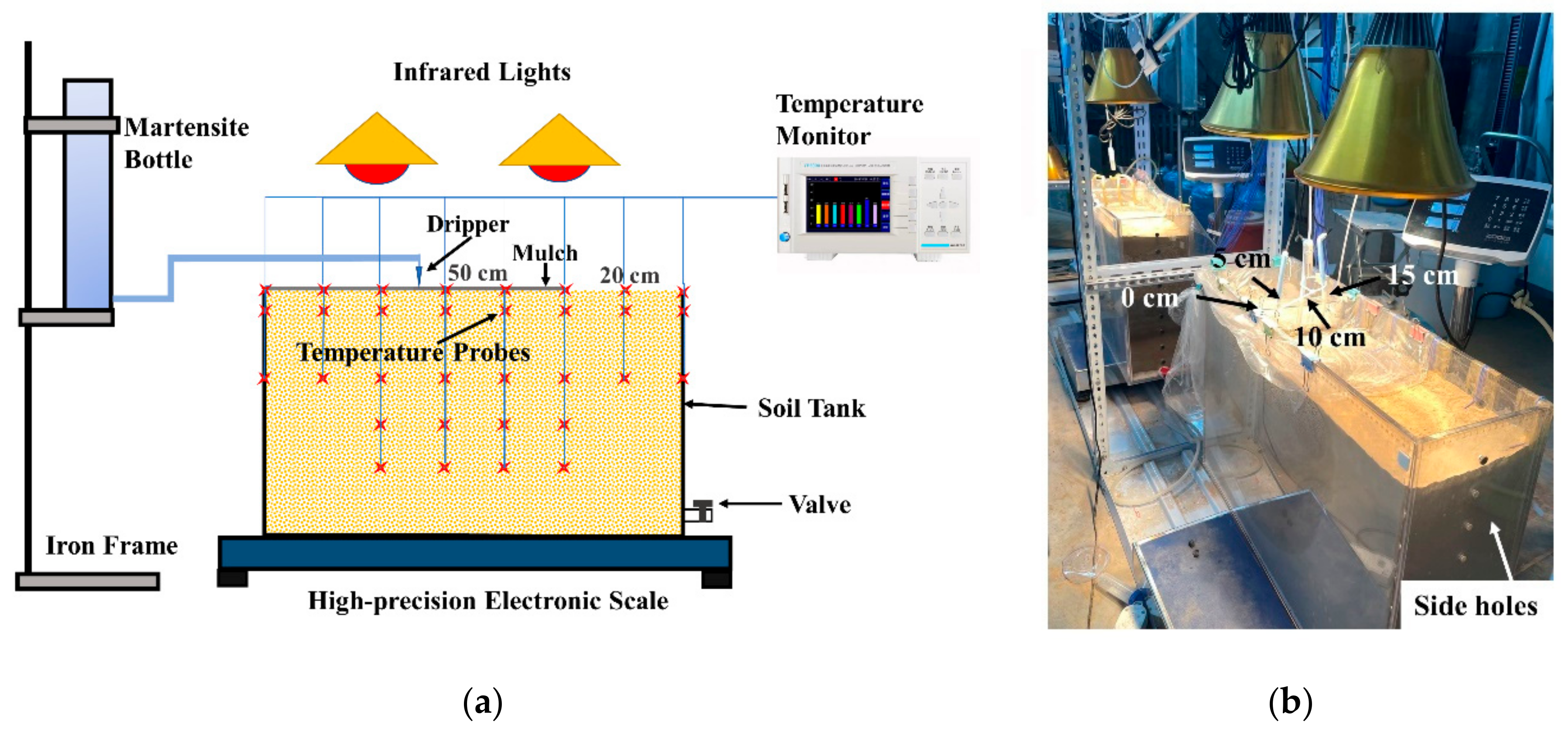
Two tank experiments involving drip irrigation under partially mulched conditions with different drip irrigation intensities were conducted in this research study. The experimental layout is shown in Figure 1. The tank size was 70 cm × 20 cm × 50 cm, with saline soil having been filled in layer by layer. To avoid the influence of trapped air during infiltration, the tanks were equipped with side holes that stayed open until the surrounding soil was saturated. The mulch and dripper were arranged based on the local farmland practice of “one mulch, four lines, and two drip irrigation zones”. The plastic mulch used in the experiment was transparent and waterproof, with a thickness of 0.01 mm.

The experiment used thermal infrared lights for heating, to simulate the sunshine situation of southern Xinjiang, with similar durations of heating each day. The combination of the arrow shape and the pressure-compensating dripper ensured the stable flow rate in this experiment. A martensite bottle provided water and the soil was irrigated with three drippers simultaneously, which were arranged at 5, 10, and 15 cm along the direction of the irrigation pipe, as shown in Figure 2a.

The soil was collected from the 0 to 40 cm of salinized fallow farmland in Aksu Prefecture, in the Xinjiang Uygur Autonomous Region (81°11′42″ E, 40°37′27″ N), where the soil salinization problem is serious. The soil texture was sandy loam, with low fertility and high soil salinity. The soil was mailed to the experimental site and was sieved, naturally dried, and fully mixed to bring it to homogeneity. The initial soil bulk density, ${\mathsf{\rho }}_{\mathrm{b}}$, was measured as 1.55 ${\mathrm{g} \mathrm{cm}}^{-3}$. The initial volumetric water content, ${\mathsf{\theta }}_0$, was 0.05 ${\mathrm{cm}}^3{ \mathrm{cm}}^{-3}$, and the initial soil salinity, ${\mathrm{S}}_0$, was 9.41 ${\mathrm{g} \mathrm{kg}}^{-1}$.

Figure 1. Layout of the mulched drip-irrigation system in the indoor soil tank: (a) Sketch map of design; (b) photograph of equipment.

Figure 1. Layout of the mulched drip-irrigation system in the indoor soil tank: (a) Sketch map of design; (b) photograph of equipment.

Two drip-irrigation treatments were established in the experiment, with different drip irrigation intensities (i.e., mostly low W1 and mostly high W2). The drip irrigation salinity was 1.6 ${\mathrm{g} \mathrm{L}}^{-1}$. They had the same total irrigation quantities. The irrigation schedule is shown in

Table 1. Irrigation schedules.

Time (d)		1	4	7	10	13	16	19	22	25	28	$\mathrm{The} \mathrm{total} \mathrm{amount} \left(\mathrm{L}\right)$
Number of irrigation $i$-th		1	2	3	4	5	6	7	8	9	10
Irrigation amount $\left(\mathrm{L}\right)$	W1 1	4	4	4	4	4	4	3	2	1	1	31
	W2 1	5	5	5	5	5	2	1	1	1	1	31

Note: ¹ The drip-irrigation flow rate of W1 and W2 was 0.4 L/h throughout the experiment.

.

2.2. Monitoring Methods

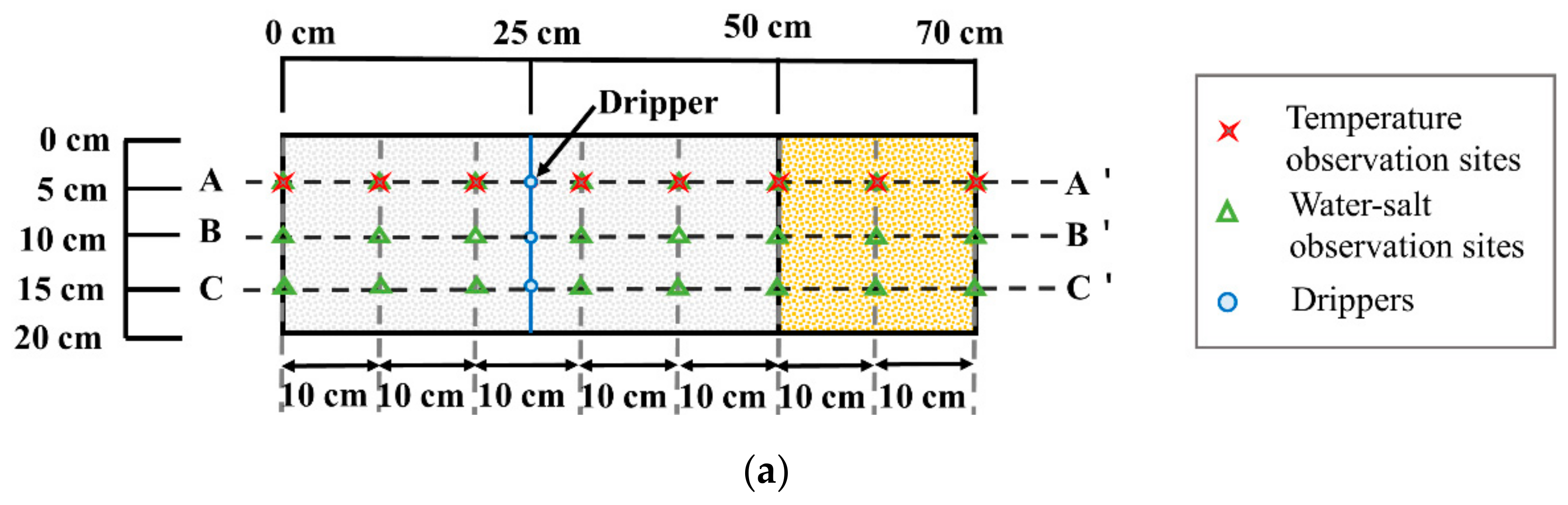
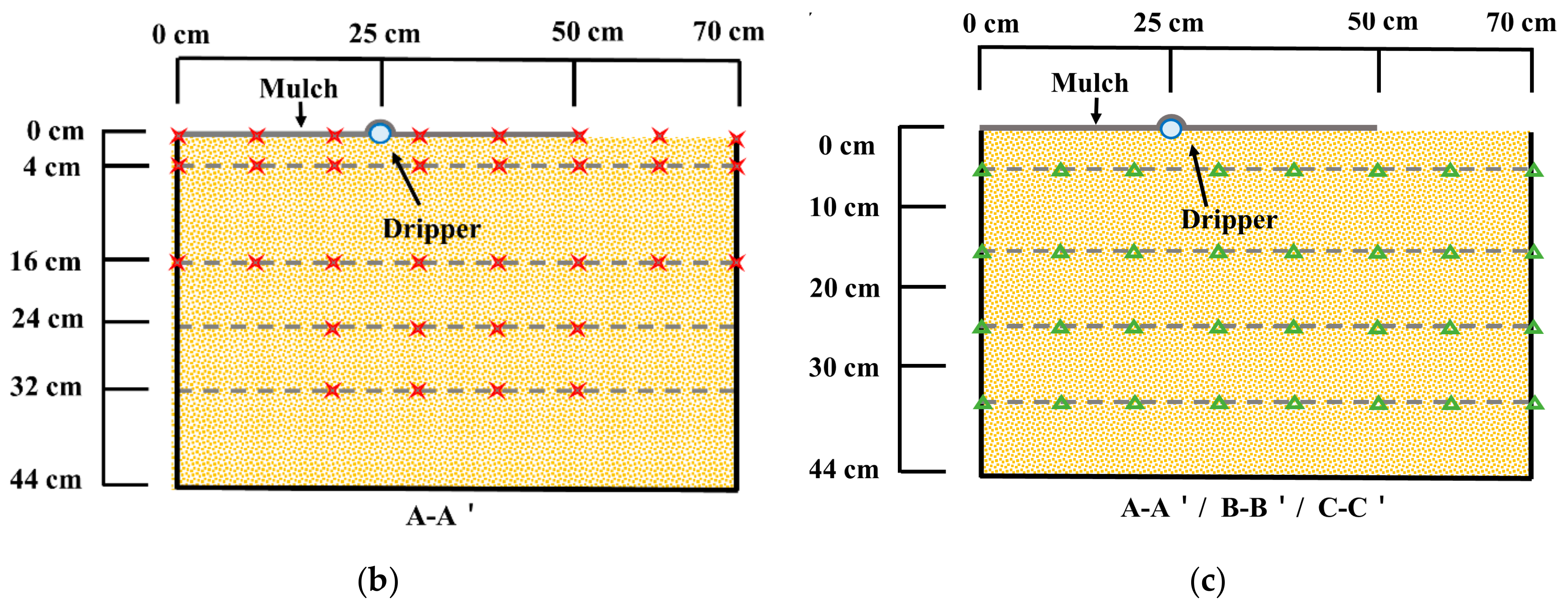
The experimental measurements included temperature monitoring and water-salt measurement. Their locations are shown in Figure 2.

The locations of the temperature probes are shown in Figure 2a,b in horizontal and vertical plane views. The temperature probes were 0.5 mm in diameter to avoid disturbing the soil, and they were connected to thermocouple wires that were wrapped in insulating plastic. The wires were connected to the monitor (as shown in Figure 1a), to collect and automatically record the temperature data each minute. The temperature monitor (YP5008G, YONGPENG, Zhongshan, China, monitoring range of −55–400 °C) was calibrated to within 0.5% using an ice–water mixture and boiling water.

The soil’s water content was measured at the end of the experiment. The locations are shown in Figure 2c in the vertical plane view. Note that the three replications in accordance with the three drippers’ locations in the horizontal view (Figure 2a). The oven-drying method was used to measure the soil water content by mass, which was converted to volumetric water content by multiplying the bulk density ${\mathsf{\rho }}_{\mathrm{b}}$.

The conductivity value ${(\mathrm{EC}}_{1:5})$ was measured by a conductivity meter (FE38, Mettler Toledo, Shanghai, China), according to the extracts with a 1:5 soil water ratio, in order to quantify the soil salt distribution at the end of the experiment. The Mettler Toledo standard solution ${(1413 \mathsf{\mu }\mathrm{S} \mathrm{cm}}^{-1})$ was used for calibration, with the error being about 3%. The soil salinity in dry soil was calculated based on Equation (1), which has been proven suitable for this kind of soil [34]:

$$\mathrm{S}={0.0037 \ast \mathrm{EC}}_{1:5}+1.0291$$

(1)

where $\mathrm{S}$ is the soil salinity in dry soil $({\mathrm{g} \mathrm{kg}}^{-1}$), and ${\mathrm{EC}}_{1:5}$ is the electrical conductivity value ${(\mathsf{\mu }\mathrm{S} \mathrm{cm}}^{-1})$.

High-precision electronic scales (ZOGGI, Jinhua, China, accuracy within 0.1%) were set under the soil tank to record the hourly mass change, which was used to track the evaporation loss from the soil tank.

Figure 2. Locations of the observation sites: (a) Temperature monitoring and water-salt observation sites in horizontal plane view; (b) temperature monitoring points in vertical plane view; (c) water-salt observation sites in vertical plane view.

Figure 2. Locations of the observation sites: (a) Temperature monitoring and water-salt observation sites in horizontal plane view; (b) temperature monitoring points in vertical plane view; (c) water-salt observation sites in vertical plane view.

2.3. Model Introduction

HYDRUS-2D was applied for the related simulations. HYDRUS-2D was widely used to simulate 2D water, salt, and heat transport in various circumstances of porous medium.

2.3.1. Equation of Water Transport

In HYDRUS-2D, Richard’s equation is used to describe soil water movement [35]:

$$\frac{\partial \mathsf{\theta }}{\partial \mathrm{t}}=\frac{\partial }{\partial \mathrm{x}}\left[\mathrm{K}\left(\mathsf{\theta }\right)\frac{\partial \mathrm{h}}{\partial \mathrm{x}}\right]+\frac{\partial }{\partial \mathrm{z}}\left[\mathrm{K}\left(\mathsf{\theta }\right)\frac{\partial \mathrm{h}}{\partial \mathrm{z}}\right]+\frac{\partial \mathrm{K}\left(\mathsf{\theta }\right)}{\partial \mathrm{z}}{+\mathrm{s}}_{\mathrm{w}}$$

(2)

where θ is the soil volume water content ${(\mathrm{cm}}^3{ \mathrm{cm}}^{-3})$, t is the time (h), h is the pressure, and $\mathrm{K}\left(\mathsf{\theta }\right)$ is unsaturated and soil water conductivity ${(\mathrm{cm} \mathrm{h}}^{-1})$, which can be obtained from the saturated water content of soil ${\mathrm{K}}_{\mathrm{s}}{ (\mathrm{cm} \mathrm{h}}^{-1})$. ${\mathrm{s}}_{\mathrm{w}}$ is the water source term ${(\mathrm{h}}^{-1})$, caused by drip irrigation. x and z are the coordinates in the horizontal and vertical (positive upwards) directions (cm), respectively.

The van Genuchten–Mualem function [36] was applied to estimate the soil water properties as follows,

$$\mathsf{\theta }\left(\mathrm{h}\right){=\mathsf{\theta }}_{\mathrm{r}}+\frac{{\mathsf{\theta }}_{\mathrm{s}}-{\mathsf{\theta }}_{\mathrm{r}}}{{\left(1+{\left|\mathsf{\alpha }\mathrm{h}\right|}^{\mathrm{n}}\right)}^{\mathrm{m}}}$$

(3)

$$\mathrm{K}\left(\mathrm{h}\right){=\mathrm{K}}_{\mathrm{s}}{\mathrm{S}}_{\mathrm{e}}^{\mathrm{l}}{\left[1-\left(1-{\mathrm{S}}_{\mathrm{e}}^{\frac{1}{\mathrm{m}}}\right)\right]}^2$$

(4)

$${\mathrm{S}}_{\mathrm{e}}=\frac{\mathsf{\theta }\left(\mathrm{h}\right)}{{\mathsf{\theta }}_{\mathrm{s}}{-\mathsf{\theta }}_{\mathrm{r}}}, \mathrm{m}=1-\frac{1}{\mathrm{n}}, \mathrm{n} > 1$$

(5)

where ${\mathsf{\theta }}_{\mathrm{s}}$ is saturated water content (${\mathrm{cm}}^3{ \mathrm{cm}}^{-3}$), ${\mathsf{\theta }}_{\mathrm{r}}$ is residual water content (${\mathrm{cm}}^3{ \mathrm{cm}}^{-3}$), α and n are shape parameters, l is pore connectivity parameter, ${\mathrm{S}}_{\mathrm{e}}$ is saturated soil. The values of water characteristic parameters are shown in Table 2.

Note that the van Genuchten–Mualem function was further modified by considering the air-entry value, which could more accurately simulate the water flow, especially in heavy soil (e.g., loam and clay) [37]. The corresponding updated function with a default air-entry value of 2 cm was provided in HYDRUS-2D. However, because the air-entry value cannot be calibrated in HYDRUS-2D and our soil texture tended to be light (sandy loam), in this study we used the original van Genuchten–Mualem function. The impact of the two functions on water flow and related salt migration in these experimental conditions will be studied in future.

2.3.2. Solute Transport Equation

For highly salinized soil, salt migration may involve complex processes includingsalt adsorption–desorption and precipitation–dissolution. Compared with the advection speed, these salt migration processes were relatively slow, so they could be grouped together as part of a non-equilibrium kinetic absorption term.

Based on the advective dispersive equation (ADE), the partial differential equation represents the non-equilibrium chemical transport of solutes involving the sequence first-order decay chain in HYDRUS-2D [38]:

$$\begin{array}{l}\frac{\partial \mathsf{\theta }\mathrm{c}}{\partial \mathrm{t}}+\frac{\partial \mathsf{\rho }\mathrm{s}}{\partial \mathrm{t}}=\frac{\partial }{\partial \mathrm{x}}\left[{\mathsf{\theta }\mathrm{D}}_0\frac{\partial \mathrm{c}}{\partial \mathrm{x}}\right]+\frac{\partial }{\partial \mathrm{z}}\left[{\mathsf{\theta }\mathrm{D}}_0\frac{\partial \mathrm{c}}{\partial \mathrm{z}}\right]-\frac{\partial \left({\mathrm{q}}_{\mathrm{x}}\mathrm{c}\right)}{\partial \mathrm{x}}-\frac{\partial \left({\mathrm{q}}_{\mathrm{z}}\mathrm{c}\right)}{\partial \mathrm{z}}+{\mathrm{s}}_{\mathrm{w}}{\mathrm{c}}_{\mathrm{r}}\\ \hspace{1em}\hspace{1em}\hspace{1em}\hspace{1em}\hspace{1em}\hspace{1em}\hspace{1em}-\left({\mathsf{\mu }}_{\mathrm{S}}{+\mathsf{\mu }}_{\mathrm{S}}^{\prime }\right){\mathsf{\rho }}_{\mathrm{b}}\mathrm{s} -\left({\mathsf{\mu }}_{\mathrm{w}}{+\mathsf{\mu }}_{\mathrm{w}}^{\prime }\right){\mathsf{\theta }\mathrm{c}+\mathsf{\gamma }}_{\mathrm{S}}{\mathsf{\rho }}_{\mathrm{b}}{+\mathsf{\gamma }}_{\mathrm{w}}\mathsf{\theta }\end{array}$$

(6)

where c is the solute concentration (${\mathrm{mg} \mathrm{cm}}^{-3}$), ${\mathrm{q}}_{\mathrm{x}}$ and ${\mathrm{q}}_{\mathrm{z}}$ are water flux amounts in the x and z directions, respectively ${(\mathrm{cm} \mathrm{h}}^{-1})$, ${\mathrm{D}}_0$ is the saturated–unsaturated hydrodynamic dispersion coefficient (${\mathrm{cm}}^{2 }{ \mathrm{h}}^{-1}$), ${\mathrm{c}}_{\mathrm{r}}$ is the concentration of irrigation water (${\mathrm{mg} \mathrm{cm}}^{-3}$), ${\mathsf{\mu }}_{\mathrm{S}}$ and ${\mathsf{\mu }}_{\mathrm{w}}$ are the first-order rate constants of the solid phase and liquid phase (${\mathrm{h}}^{-1}$), ${\mathsf{\mu }}_{\mathrm{S}}^{\prime }{, \mathsf{\mu }}_{\mathrm{w}}^{\prime }$ are the first order rate constants of the solid phase and liquid phase in the solute decay chain (${\mathrm{h}}^{-1}$), ${\mathsf{\gamma }}_{\mathrm{S}}$ and ${\mathsf{\gamma }}_{\mathrm{w}}$ are the zero-order rate constant of the solid phase and liquid phase (${\mathrm{h}}^{-1}$), ${\mathsf{\rho }}_{\mathrm{b}}$ is the soil bulk density of soil (${\mathrm{g} \mathrm{cm}}^{-3}$), $\mathrm{s}$ is the adsorption quantity (${\mathrm{mg} \mathrm{g}}^{-1}$).

The saturated–unsaturated hydrodynamic dispersion coefficient ${\mathrm{D}}_0$ was calculated according to Equation (7):

$${\mathsf{\theta }\mathrm{D}}_{0 }{=\mathrm{D}}_{\mathrm{T}}\left|\mathrm{q}\right|+\left({\mathrm{D}}_{\mathrm{L}}-{\mathrm{D}}_{\mathrm{T}}\right)\frac{{\mathrm{q}}_{\mathrm{x}}{\mathrm{q}}_{\mathrm{z}}}{\left|\mathrm{q}\right|}{+\mathsf{\theta }\mathrm{D}}_{\mathrm{w}}{\mathsf{\tau }}_{\mathrm{w}}+\left({\mathrm{D}}_{\mathrm{L}} {- \mathrm{D}}_{\mathrm{T}}\right)\frac{{\mathrm{q}}_{\mathrm{z}}{}^2}{\left|\mathrm{q}\right|}$$

(7)

where ${\mathsf{\tau }}_{\mathrm{w}}$ is the liquid phase bending coefficient, ${\mathrm{D}}_{\mathrm{w}}$ refers to the diffusion coefficient of solute molecules in water (${\mathrm{cm}}^2{ \mathrm{h}}^{-1}$), ${\mathrm{D}}_{\mathrm{L}}$ and ${\mathrm{D}}_{\mathrm{T}}$ are the longitudinal and transverse dispersion (cm), respectively; other parameters were the same as before.

Considering the adsorption effect of soil on salt, a two-point adsorption model was applied to analyze the non-equilibrium adsorption reaction. Adsorption points were divided into non-equilibrium adsorption point ${\mathrm{s}}_0{}^{\mathrm{k}}$ and instantaneous equilibrium adsorption point ${\mathrm{s}}_0{}^{\mathrm{e}}$ [39], expressed in Equation (8):

$${\mathrm{s}}_0{=\mathrm{s}}_0{}^{\mathrm{k}}{+\mathrm{s}}_0{}^{\mathrm{e} }{=\mathrm{s}}_0{}^{\mathrm{k}}{+\mathrm{fs}}_0$$

(8)

where f is the ratio of instantaneous adsorption points to all adsorption points.

An unbalanced interaction occurred between the concentration of dissolution $\mathrm{c}$ (${\mathrm{mg} \mathrm{cm}}^{-3}$) and adsorption $\mathrm{s}$ (${\mathrm{mg} \mathrm{g}}^{-1}$). The linear isothermal adsorption equation (Freundlich equation) was used to describe the relationship (β = 1, $\mathsf{\eta }=0$). The relation equation between s and c was established as follows:

$${\mathrm{s}=\mathrm{k}}_{\mathrm{s}}\mathrm{c}$$

(9)

$$\frac{\partial \mathrm{s}}{\partial \mathrm{t}}=\frac{{\mathrm{k}}_{\mathrm{s}}\partial \mathrm{c}}{\partial \mathrm{t}}$$

(10)

where ${\mathrm{k}}_{\mathrm{s}}$ is the empirical coefficient (${\mathrm{cm}}^3{ \mathrm{g}}^{-1}$); its value is shown in Table 2.

Because non-equilibrium point adsorption ${\mathrm{s}}^{\mathrm{k}}$ is assumed to be a first-order dynamic process, Equation (11) is proposed [40]:

$$\frac{\partial {\mathrm{s}}^{\mathrm{k}}}{\partial \mathrm{t}}={\mathsf{\alpha }}^{\prime } \left[\left(1 - \mathrm{f}\right){\mathrm{k}}_{\mathrm{s}}\mathrm{c} -{ \mathrm{s}}^{\mathrm{k}}\right]+\left(1 - \mathrm{f}\right){\mathsf{\gamma }}_{\mathrm{S}}-{ (\mathsf{\mu }}_{\mathrm{S}}{+\mathsf{\mu }}_{\mathrm{S}}^{\prime }{)\mathrm{s}}^{\mathrm{k}}$$

(11)

where ${\mathsf{\alpha }}^{\prime }$ is the first-rate constant of the solute (${\mathrm{h}}^{-1}$).

2.3.3. Heat Transport Equation

The 2D heat conduction equation and related parameter calculation equation can be expressed as follows [41]:

$$\mathrm{C}\left(\mathsf{\theta }\right)\frac{\partial \mathrm{T}}{\partial \mathrm{t}}=\frac{\partial }{\partial \mathrm{x}}\left[{\mathrm{K}}_{\mathrm{h}}\left(\mathsf{\theta }\right)\frac{\partial \mathrm{T}}{\partial \mathrm{x}}\right]+\frac{\partial }{\partial \mathrm{z}}\left[{\mathrm{K}}_{\mathrm{h}}\left(\mathsf{\theta }\right)\frac{\partial \mathrm{T}}{\partial \mathrm{z}}\right]-{ \mathrm{C}}_{\mathrm{w}}{\mathrm{q}}_{\mathrm{x}}\frac{\partial \mathrm{T}}{\partial \mathrm{x}}-{ \mathrm{C}}_{\mathrm{w}}{\mathrm{q}}_{\mathrm{z}}\frac{\partial \mathrm{T}}{\partial \mathrm{z}}+{\mathrm{C}}_{\mathrm{w}}{\mathrm{s}}_{\mathrm{w}}{\mathrm{T}}_{\mathrm{w}}$$

(12)

where $\mathrm{C}\left(\mathsf{\theta }\right)$ is the soil volumetric heat capacity (${\mathrm{J} \mathrm{m}}^{-3} {℃}^{-1}$), ${\mathrm{K}}_{\mathrm{h}}\left(\mathsf{\theta }\right)$ is the soil sensible heat conductivity coefficient (${\mathrm{W} \mathrm{m}}^{-1} {℃}^{-1}$), ${\mathrm{C}}_{\mathrm{w}}$ is the liquid volume heat capacity (${\mathrm{J} \mathrm{m}}^{-3} {℃}^{-1}$), ${\mathrm{T}}_{\mathrm{w}}$ is the temperature of irrigation water.

The sensible heat conductivity of soil ${\mathrm{K}}_{\mathrm{h}}\left(\mathsf{\theta }\right)$ was calculated according to Equation (13) [42]:

$${\mathrm{K}}_{\mathrm{h}}\left(\mathsf{\theta }\right){=\mathsf{\lambda }}_{\mathrm{T}}{\mathrm{C}}_{\mathrm{w}}\left|\mathrm{q}\right|+\left({\mathsf{\lambda }}_{\mathrm{L}}-{\mathsf{\lambda }}_{\mathrm{T}}\right){\mathrm{C}}_{\mathrm{w}}\frac{{\mathrm{q}}_{\mathrm{x}}{\mathrm{q}}_{\mathrm{z}}}{\left|\mathrm{q}\right|}{+\mathsf{\lambda }}_0\left(\mathsf{\theta }\right)+\left({\mathsf{\lambda }}_{\mathrm{L}}-{\mathsf{\lambda }}_{\mathrm{T}}\right){\mathrm{C}}_{\mathrm{w}}\frac{{\mathrm{q}}_{\mathrm{z}}{}^2}{\left|\mathrm{q}\right|}$$

(13)

where ${\mathsf{\lambda }}_{\mathrm{L}}$ and ${\mathsf{\lambda }}_{\mathrm{T}}$ are the longitudinal and transverse thermal conductivity (cm), respectively. ${\mathsf{\lambda }}_0\left(\mathsf{\theta }\right)$ refers to the thermal conductivity coefficient (${\mathrm{W} \mathrm{m}}^{-1}{ \mathrm{K}}^{-1}$).

The thermal conductivity coefficient ${\mathsf{\lambda }}_0\left(\mathsf{\theta }\right)$ was calculated according to Equation (14) [43]:

$${\mathsf{\lambda }}_0\left(\mathsf{\theta }\right){=\mathrm{b}}_1{+\mathrm{b}}_2{\mathsf{\theta }+\mathrm{b}}_3{\mathsf{\theta }}^{0.5}$$

(14)

where ${\mathrm{b}}_1{, \mathrm{b}}_2{, \mathrm{b}}_3$ are the empirical coefficients (${\mathrm{W} \mathrm{m}}^{-1}{ \mathrm{K}}^{-1}$). The values are shown in Table 2.

2.3.4. Initial and Boundary Conditions

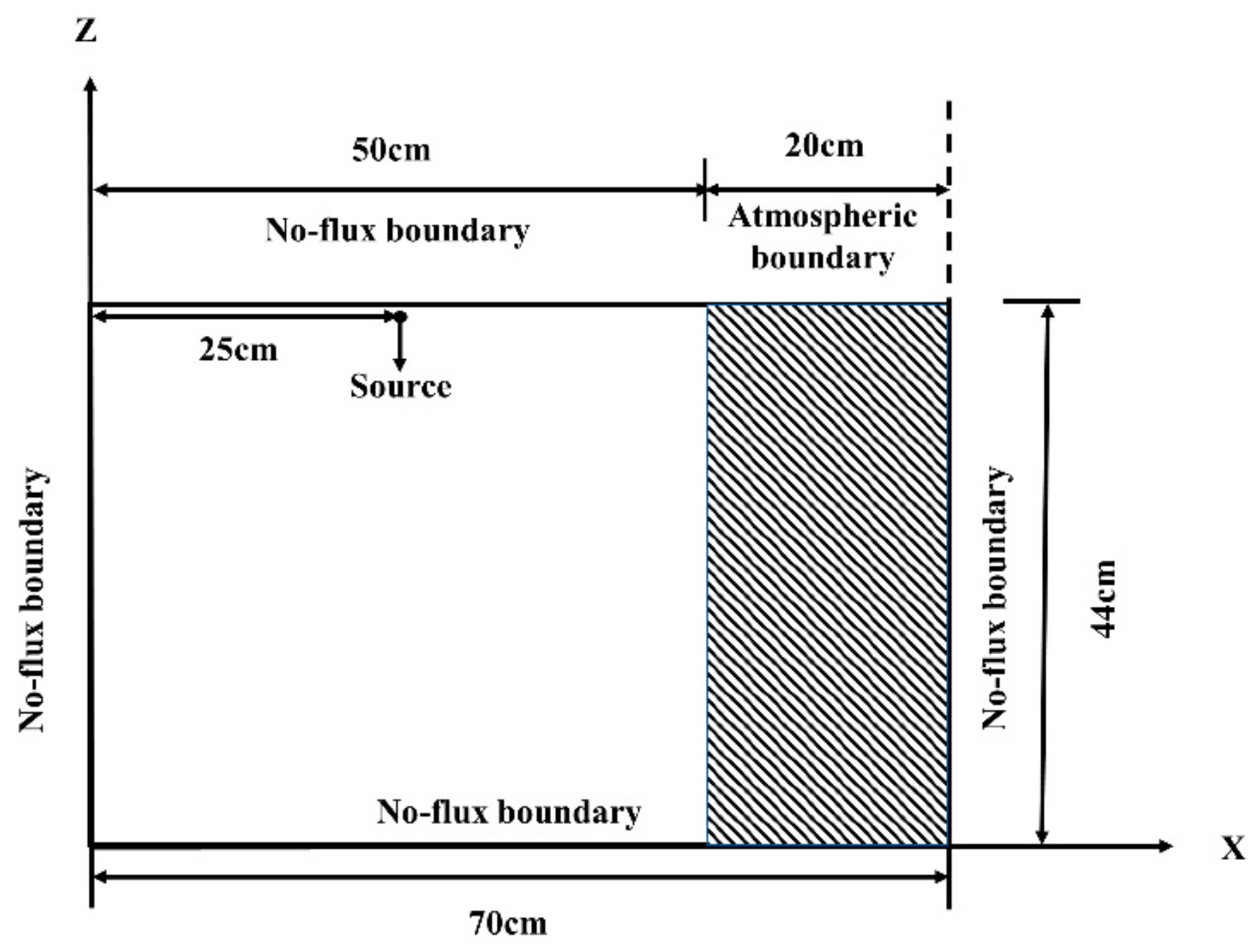
The origin of coordinates (x = 0, z = 0) was located at the lower left corner of the soil tank. The direction perpendicular to the irrigation pipe was the horizontal (x) direction, and the upward direction along the tank edge was the vertical (z) direction, as shown in Figure 3. The simulated area was defined as a section with a length of 70 cm and a height of 44 cm. Because HYDRUS-2D allowed only a maximum of two inputs of time-varying boundary conditions for temperature, for the purpose of describing the temperature difference in the upper boundary, the first-boundary conditions with the measured temperature were set for the high and low temperature zones, respectively. Meanwhile, irrigation was assumed to proceed from an internal source close to the upper boundary.

The initial soil water content, salinity, and temperature were assumed to be evenly distributed throughout the entire section. The initial boundaries are shown as follows:

$$\left\{\begin{array}{c}\mathsf{\theta }\left(\mathrm{x},\mathrm{z},\mathrm{t}\right){=\mathsf{\theta }}_0\left(\mathrm{x},\mathrm{z},\mathrm{t}\right)\\ \mathrm{C}\left(\mathrm{x},\mathrm{z},\mathrm{t}\right){=\mathrm{C}}_0\left(\mathrm{x},\mathrm{z},\mathrm{t}\right)\\ \mathrm{T}\left(\mathrm{x},\mathrm{z},\mathrm{t}\right){=\mathrm{T}}_0\left(\mathrm{x},\mathrm{z},\mathrm{t}\right)\\ 0 \mathrm{cm} \le \mathrm{x} \le 70 \mathrm{cm},0 \mathrm{cm} \le \mathrm{z} \le 44 \mathrm{cm}, \mathrm{t}=0 \mathrm{h}\end{array}\right.$$

(15)

where according to the experiment setup, soil water content ${\mathsf{\theta }}_0$ was 0.05 ${\mathrm{cm}}^3{ \mathrm{cm}}^{-3}$ and the initial solute concentration ${\mathrm{C}}_0$ was 291.47 ${\mathrm{mg} \mathrm{cm}}^{-3}$. ${\mathrm{T}}_0$ was based on the measured value at the initial experimental stage.

The upper boundary was divided into two parts (i.e., 0 cm ≤ x ≤ 50 cm, and 50 cm ≤ x ≤ 70 cm) in accordance with the mulched and un-mulched soil areas. The mulched soil area was set as a no-flux boundary, and the un-mulched soil area was set as an atmospheric boundary with evaporation. The solute transport boundaries were all zero flux; the dripper was regarded as a source. The heat transport boundary was of the first type of boundary condition. The upper boundary was divided into a high temperature zone (25–70 cm) and a low temperature zone (0–25 cm) according to the measured results. The upper boundary conditions were:

$$-\mathrm{K}\left(\mathsf{\theta }\right)\frac{\partial \mathrm{h}}{\partial \mathrm{z}}-\mathrm{K}\left(\mathsf{\theta }\right)=\left\{\begin{array}{c}0 0 \mathrm{cm} \le \mathrm{x} \le 50 \mathrm{cm}, \mathrm{z}=44 \mathrm{cm}, \mathrm{t} \ge 0 \mathrm{h}\\ \\ \mathrm{E}\left(\mathrm{t}\right) 50 \mathrm{cm} < \mathrm{x} \le 70 \mathrm{cm}, \mathrm{z}=44 \mathrm{cm}, \mathrm{t} \ge 0 \mathrm{h}\end{array}\right.$$

(16)

$$-{\mathsf{\theta }\mathrm{D}}_0\frac{\partial \mathrm{c}}{\partial \mathrm{z}}{+\mathrm{q}}_{\mathrm{z}}\mathrm{c}=0, \mathrm{z}=44 \mathrm{cm}, \mathrm{t} \ge 0 \mathrm{h}$$

(17)

$$\mathrm{T}\left(\mathrm{x},\mathrm{z},\mathrm{t}\right)=\left\{\begin{array}{c}{\mathrm{T}}_1\left(\mathrm{x},\mathrm{z},\mathrm{t}\right), 0 \mathrm{cm} \le \mathrm{x} \le 25 \mathrm{cm}, \mathrm{z}=44 \mathrm{cm}\\ {\mathrm{T}}_2\left(\mathrm{x},\mathrm{z},\mathrm{t}\right), 25 \mathrm{cm} < \mathrm{x} \le 70 \mathrm{cm}, \mathrm{z}=44 \mathrm{cm}\end{array}\right., \mathrm{t} \ge 0 \mathrm{h}$$

(18)

where E (t) is the evaporation flux, ${\mathrm{T}}_1\left(\mathrm{x},\mathrm{z},\mathrm{t}\right)$ is the temperature in the low temperature zone, and ${\mathrm{T}}_2\left(\mathrm{x},\mathrm{z},\mathrm{t}\right)$ is the temperature in the high temperature zone.

All boundaries except for the upper boundary were set as zero-flux boundaries, and the bottom boundary conditions were as follows:

$$-\mathrm{K}\left(\mathsf{\theta }\right)\frac{\partial \mathrm{h}}{\partial \mathrm{z}}-\mathrm{K}\left(\mathsf{\theta }\right)=0, 0 \mathrm{cm} \le \mathrm{x} \le 70 \mathrm{cm}, \mathrm{z}=0 \mathrm{cm}, \mathrm{t} \ge 0 \mathrm{h}$$

(19)

$$-{\mathsf{\theta }\mathrm{D}}_0\frac{\partial \mathrm{c}}{\partial \mathrm{z}}{+\mathrm{q}}_{\mathrm{z}}\mathrm{c}=0, \mathrm{z}=0 \mathrm{cm}, \mathrm{t} \ge 0 \mathrm{h}$$

(20)

$$-{\mathrm{K}}_{\mathrm{h}}\left(\mathsf{\theta }\right)\frac{\partial \mathrm{T}}{\partial \mathrm{z}}{+\mathrm{C}}_{\mathrm{w}}{\mathrm{q}}_{\mathrm{z}}\mathrm{T}=0, \mathrm{z}=0 \mathrm{cm}, \mathrm{t} \ge 0 \mathrm{h}$$

(21)

2.3.5. Parameters and Model Calibration/Validation

The model was calibrated using W2 and was validated with W1. The calibration strategy included provision of parameters related to soil hydraulic properties, salt transport, and heat transport, based on reference, measurement, or empirical values. Then the measured data of W2 were used for calibration, and verification by the W1 process was conducted. The final parameters applied in this study are shown in the Table 2.

Table 2. Values of soil parameters for water, salt, and heat transport under partially mulched conditions with drip irrigation.

Parameters				Value	Source
Soil characteristic parameter	Soil particle composition	Sand	$\%$	26.252	Measured via experiment
		Silt	$\%$	70.858
		Clay	$\%$	2.89
	${\mathsf{\rho }}_{\mathrm{b}}$		${\mathrm{g} \mathrm{cm}}^{-3}$	1.55
Soil hydraulic parameters	${\mathsf{\theta }}_{\mathrm{r}}$		${\mathrm{cm}}^3{ \mathrm{cm}}^{-3}$	0.0353	Rosetta pedotransfer functions [44]
	${\mathsf{\theta }}_{\mathrm{s}}$		${\mathrm{cm}}^3{ \mathrm{cm}}^{-3}$	0.42
	$\mathsf{\alpha }$		${\mathrm{cm}}^{-1}$	0.0072
	$\mathrm{n}$		$-$	1.6613
	${\mathrm{K}}_{\mathrm{s}}$		${\mathrm{cm} \mathrm{h}}^{-1}$	1.875
	l		$-$	0.5
Solute transport parameters	${\mathrm{D}}_{\mathrm{L}}$		$\mathrm{Cm}$	26	Calibrated
	${\mathrm{D}}_{\mathrm{T}}$		$\mathrm{Cm}$	$1$
	$\mathrm{f}$		$-$	$0.9$
	${\mathrm{D}}_{\mathrm{W}}$		${\mathrm{cm}}^{2 }{\mathrm{h}}^{-1}$	$0.09$
	${\mathrm{K}}_{\mathrm{d}}$		${\mathrm{cm}}^3{ \mathrm{g}}^{-1}$	0.6
	$\mathsf{\beta }$		$-$	1
	${\mathsf{\mu }}_{\mathrm{w}}$		${\mathrm{h}}^{-1}$	$2\times {10}^{-4}$
	${\mathsf{\mu }}_{\mathrm{S}}$		${\mathrm{h}}^{-1}$	$4.16\times {10}^{-4}$
	${\mathsf{\mu }}_{\mathrm{w}}^{\prime }$		${\mathrm{h}}^{-1}$	$2\times {10}^{-4}$
	${\mathsf{\mu }}_{\mathrm{S}}^{\prime }$		${\mathrm{h}}^{-1}$	$2.92\times {10}^{-4}$
	${\mathsf{\gamma }}_{\mathrm{w}}$		${\mathrm{mg} \mathrm{cm}}^{-3}{ \mathrm{h}}^{-1}$	$9\times {10}^{-3}$
	${\mathsf{\gamma }}_{\mathrm{S}}$		${\mathrm{h}}^{-1}$	$7.33\times {10}^{-3}$
	${\mathsf{\alpha }}^{\prime }$		${\mathrm{h}}^{-1}$	0.05
Heat transport parameters	${\mathrm{b}}_1$		${\mathrm{W} \mathrm{m}}^{-1}{ \mathrm{K}}^{-1}$	−0.5519	Wang et al. [45]
	${\mathrm{b}}_2$		${\mathrm{W} \mathrm{m}}^{-1}{ \mathrm{K}}^{-1}$	−4.05
	${\mathrm{b}}_3$		${\mathrm{W} \mathrm{m}}^{-1}{ \mathrm{K}}^{-1}$	3.75
	${\mathrm{C}}_{\mathrm{w}}$		${\mathrm{J} \mathrm{m}}^{-3} {℃}^{-1}$	$4.16\times {10}^6$	Pan et al. [46]
	${\mathrm{C}}_{\mathrm{n}}$		${\mathrm{J} \mathrm{m}}^{-3} {℃}^{-1}$	$2.23\times {10}^6$
	${\mathsf{\lambda }}_{\mathrm{L}}$		$\mathrm{cm}$	$5$	Hu et al. [47]
	${\mathsf{\lambda }}_{\mathrm{T}}$		$\mathrm{cm}$	1

Table 2. Values of soil parameters for water, salt, and heat transport under partially mulched conditions with drip irrigation.

Parameters				Value	Source
Soil characteristic parameter	Soil particle composition	Sand	$\%$	26.252	Measured via experiment
		Silt	$\%$	70.858
		Clay	$\%$	2.89
	${\mathsf{\rho }}_{\mathrm{b}}$		${\mathrm{g} \mathrm{cm}}^{-3}$	1.55
Soil hydraulic parameters	${\mathsf{\theta }}_{\mathrm{r}}$		${\mathrm{cm}}^3{ \mathrm{cm}}^{-3}$	0.0353	Rosetta pedotransfer functions [44]
	${\mathsf{\theta }}_{\mathrm{s}}$		${\mathrm{cm}}^3{ \mathrm{cm}}^{-3}$	0.42
	$\mathsf{\alpha }$		${\mathrm{cm}}^{-1}$	0.0072
	$\mathrm{n}$		$-$	1.6613
	${\mathrm{K}}_{\mathrm{s}}$		${\mathrm{cm} \mathrm{h}}^{-1}$	1.875
	l		$-$	0.5
Solute transport parameters	${\mathrm{D}}_{\mathrm{L}}$		$\mathrm{Cm}$	26	Calibrated
	${\mathrm{D}}_{\mathrm{T}}$		$\mathrm{Cm}$	$1$
	$\mathrm{f}$		$-$	$0.9$
	${\mathrm{D}}_{\mathrm{W}}$		${\mathrm{cm}}^{2 }{\mathrm{h}}^{-1}$	$0.09$
	${\mathrm{K}}_{\mathrm{d}}$		${\mathrm{cm}}^3{ \mathrm{g}}^{-1}$	0.6
	$\mathsf{\beta }$		$-$	1
	${\mathsf{\mu }}_{\mathrm{w}}$		${\mathrm{h}}^{-1}$	$2\times {10}^{-4}$
	${\mathsf{\mu }}_{\mathrm{S}}$		${\mathrm{h}}^{-1}$	$4.16\times {10}^{-4}$
	${\mathsf{\mu }}_{\mathrm{w}}^{\prime }$		${\mathrm{h}}^{-1}$	$2\times {10}^{-4}$
	${\mathsf{\mu }}_{\mathrm{S}}^{\prime }$		${\mathrm{h}}^{-1}$	$2.92\times {10}^{-4}$
	${\mathsf{\gamma }}_{\mathrm{w}}$		${\mathrm{mg} \mathrm{cm}}^{-3}{ \mathrm{h}}^{-1}$	$9\times {10}^{-3}$
	${\mathsf{\gamma }}_{\mathrm{S}}$		${\mathrm{h}}^{-1}$	$7.33\times {10}^{-3}$
	${\mathsf{\alpha }}^{\prime }$		${\mathrm{h}}^{-1}$	0.05
Heat transport parameters	${\mathrm{b}}_1$		${\mathrm{W} \mathrm{m}}^{-1}{ \mathrm{K}}^{-1}$	−0.5519	Wang et al. [45]
	${\mathrm{b}}_2$		${\mathrm{W} \mathrm{m}}^{-1}{ \mathrm{K}}^{-1}$	−4.05
	${\mathrm{b}}_3$		${\mathrm{W} \mathrm{m}}^{-1}{ \mathrm{K}}^{-1}$	3.75
	${\mathrm{C}}_{\mathrm{w}}$		${\mathrm{J} \mathrm{m}}^{-3} {℃}^{-1}$	$4.16\times {10}^6$	Pan et al. [46]
	${\mathrm{C}}_{\mathrm{n}}$		${\mathrm{J} \mathrm{m}}^{-3} {℃}^{-1}$	$2.23\times {10}^6$
	${\mathsf{\lambda }}_{\mathrm{L}}$		$\mathrm{cm}$	$5$	Hu et al. [47]
	${\mathsf{\lambda }}_{\mathrm{T}}$		$\mathrm{cm}$	1

The data used for calibration and validation include the measured soil water and salt salinity at the end of the experiment, as well as the temperature, which was monitored daily during the experiment. In the calibration process, a trial-and-error method was used to obtain good consistency between the simulated data and the observed data, as applied in the other studies [48].

2.4. Statistical Analysis

The four statistical indicators were utilized to evaluate the simulation reliability of the model. The first three indicators, the mean absolute error (MAE), the root mean square error (RMSE), and the normalized mean squared error (NRMSE) were used to reflect the differences between simulated and measured values. The fourth indicator, the coefficient of determination ${(\mathrm{R}}^2)$, was used to reflect the model’s simulation performance. The calculation equations were as follows:

$$\mathrm{MAE}=\frac{{{\displaystyle \sum }}_{\mathrm{i}=1}^{\mathrm{N}}\left|{\mathrm{O}}_{\mathrm{i} }-{ \mathrm{P}}_{\mathrm{i}}\right|}{\mathrm{N}}$$

(22)

$$\mathrm{RMSE}={\left[\frac{{{\displaystyle \sum }}_{\mathrm{i}=1}^{\mathrm{N}}{\left({\mathrm{P}}_{\mathrm{i}}-{ \mathrm{O}}_{\mathrm{i}}\right)}^2}{\mathrm{N}}\right]}^{1/2}$$

(23)

$$\mathrm{NRMSE}=\frac{\mathrm{RMSE}}{\frac{{{\displaystyle \sum }}_{\mathrm{i}=1}^{\mathrm{N}}{\mathrm{P}}_{\mathrm{i}}}{\mathrm{N}}} \times 100\%$$

(24)

$${\mathrm{R}}^2=\frac{{\left[{{\displaystyle \sum }}_{\mathrm{i}=1}^{\mathrm{N}}\left({\mathrm{O}}_{\mathrm{i}}-\frac{{{\displaystyle \sum }}_{\mathrm{i}=1}^{\mathrm{N}}{\mathrm{O}}_{\mathrm{i}}}{\mathrm{N}}\right)\left({\mathrm{P}}_{\mathrm{i}}-\frac{{{\displaystyle \sum }}_{\mathrm{i}=1}^{\mathrm{N}}{\mathrm{P}}_{\mathrm{i}}}{\mathrm{N}}\right)\right]}^2}{{{\displaystyle \sum }}_{\mathrm{i}=1}^{\mathrm{N}}{\left({\mathrm{O}}_{\mathrm{i}}-\frac{{{\displaystyle \sum }}_{\mathrm{i}=1}^{\mathrm{N}}{\mathrm{O}}_{\mathrm{i}}}{\mathrm{N}}\right)}^2{{\displaystyle \sum }}_{\mathrm{i}=1}^{\mathrm{N}}{\left({\mathrm{P}}_{\mathrm{i}}-\frac{{{\displaystyle \sum }}_{\mathrm{i}=1}^{\mathrm{N}}{\mathrm{P}}_{\mathrm{i}}}{\mathrm{N}}\right)}^2}$$

(25)

where ${\mathrm{O}}_{\mathrm{i}}$ is the observed value, ${\mathrm{P}}_{\mathrm{i}}$ is the simulated value, and $\mathrm{N}$ is the number of the dataset.

3. Results and Discussion

3.1. Results of Model Calibration and Validation

The evaluation indices for model performance are shown in

Table 3. Results of the statistical analysis between measured and simulated data.

	$\mathbf{Water} \mathbf{Contents} \left({\mathbf{cm}}^3{ \mathbf{cm}}^{-3}\right)$		$\mathbf{Salinity} \left({\mathbf{g} \mathbf{kg}}^{-1}\right)$		$\mathbf{Temperature} (°\mathbf{C})$
	W1	W2	W1	W2	W1	W2
MAE	0.0051	0.0074	1.16	1.13	1.32	1.76
RMSE	0.0064	0.0092	1.48	1.52	1.60	2.16
NRMSE (%)	1.63	2.32	16.35	16.64	5.04	6.63
$R^2$	0.67	0.70	0.66	0.54	0.79	0.71

. The simulated temperature distribution was well matched with the measured data. Meanwhile, the respective simulations for the soil’s water content and salinity matched reasonably well, indicating that the model was able to simulate and reproduce the water, salt, and heat transport processes during the experiment.

The simulated data and the measured data for water and salt transport in the soil profile at the end of the experiment, and the measured data for soil temperature transport in the soil profile during irrigation, under W1 and W2 conditions, are shown in Figure 4, Figure 5, Figure 6, Figure 7, Figure 8, Figure 9 and Figure 11. Figure 4, Figure 5, Figure 6, Figure 7, Figure 8 and Figure 9 offer a comparison of simulated and measured soil water content and salinity, respectively. Figure 11 shows the spatial distribution of the average temperature for the entire experimental period, from simulation and measurement data. The overall model was relatively reliable, especially for the temperature simulation.

3.2. Water Transport under Various Irrigation Treatments

Figure 4 and Figure 5 show the simulated contours of soil water content at different stages of the experiment, for W1 and W2, respectively. An obvious difference in water content was found between the mulched soil area and the un-mulched soil area. This difference was also verified through measurement (Figure 6a,b). The water migrated from where the dripper was located, and spread in a semicircular shape (Figure 4a–c). Because the un-mulched area was further from the dripper, it took a longer time for the water to reach it. Therefore, difference in water content was always apparent between the two zones, similar to previous findings [49]. In addition, evaporation caused an increased in water loss within the un-mulched area, leading in the later stage of irrigation to the formation of an arc-shaped area of low water content centered on the un-mulched soil (i.e., Figure 4d). The contour of the simulated water content was smoother than that of the measured content, mainly because the soil was treated as ideally homogeneous in simulation, whereas in reality it was more likely to be heterogenous and preferential flow ultimately could not be avoided.

Different intensities of drip irrigation can influence soil water migration and water distribution [33,50]. In this study, water migration occurred at a lesser rate under lower intensity W1 conditions (i.e., a low amount of drip-irrigation water for the first to fifth irrigations) than for W2, according to the simulation (Figure 4 and Figure 5). Under simulated W2 conditions, water migrated to the bottom earlier and was more likely to accumulate under the mulch (Figure 5c). Because the total amount of irrigation was the same, the W2 irrigation water amount was less than that of W1 after the fifth irrigation. However, the un-mulched soil area remained in a high water-content state and maintained a stable larger rate of evaporation. The large water gradient caused the upward migration of water (i.e., Figure 5d), so the difference in water distribution at the end of the period was more obvious (Figure 6b). After the fifth irrigation, the irrigated amount of W1 was larger than that of W2, and water was concentrated in the upper layer. Under evaporation conditions, migration to the un-mulched soil area was faster and led to a greater amount of evaporation. Thus, the overall water distribution difference of W1 was less than that of W2 (Figure 6).

Figure 4. Simulated contours of soil water content under W1: (a) The middle of first irrigation; (b) the middle of third irrigation; (c) the middle of fifth irrigation; (d) at the end of experiment.

Figure 4. Simulated contours of soil water content under W1: (a) The middle of first irrigation; (b) the middle of third irrigation; (c) the middle of fifth irrigation; (d) at the end of experiment.

Figure 5. The simulated contours of soil water content under W2: (a) The middle of first irrigation; (b) the middle of third irrigation; (c) the middle of fifth irrigation; (d) at the end of experiment.

Figure 5. The simulated contours of soil water content under W2: (a) The middle of first irrigation; (b) the middle of third irrigation; (c) the middle of fifth irrigation; (d) at the end of experiment.

Figure 6. The measured 2D distribution of soil water content at the end of experiment: (a) Measured distribution under W1; (b) measured distribution under W2.

Figure 6. The measured 2D distribution of soil water content at the end of experiment: (a) Measured distribution under W1; (b) measured distribution under W2.

3.3. Salt Transport under Various Irrigation Treatments

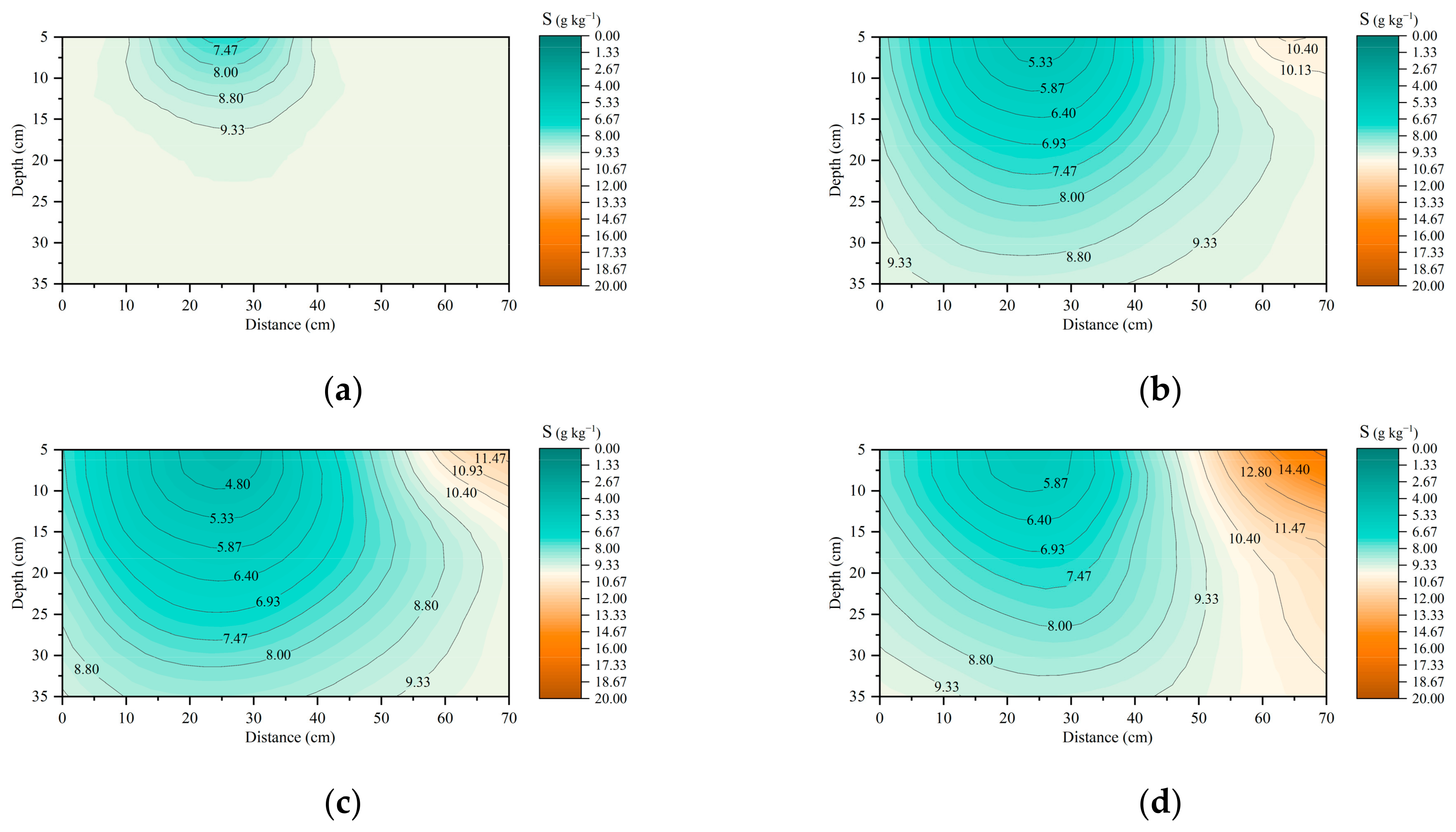
Figure 7 and Figure 8 show the simulated contours of soil salinity at different stages of the experiment for W1 and W2, respectively. In the figures, the color white corresponded to the initial soil salinity (9.41 ${\mathrm{g} \mathrm{kg}}^{-1}$), while blue and brown colors represent the desalination and salt accumulation areas, respectively. A large difference in soil salinity was obvious between the mulched and un-mulched soil areas; this difference was also verified through the measurements (Figure 9a,b). The salt accumulated in the un-mulched soil area, especially at shallower depths. Meanwhile, the desalination effect under the mulch was larger at shallower soil depths, especially for the area close to the dripper. This phenomenon was consistently found in the field experiment [5,22].

The differences between simulation and measurements were mainly found in the desalination area below the dripper. The desalination area obtained from the simulation (Figure 7d and Figure 8d) showed a lesser degree of desalination (the simulated soil salinity was around 5.29–5.81 ${\mathrm{g} \mathrm{kg}}^{-1}$ below the dripper, whereas the measured salinity indicated in Figure 9 was around 2.39–3.03 ${\mathrm{g} \mathrm{kg}}^{-1}$). This was because the soil surface in the experiment was not flat, but instead featured a pit formed by the impact of water droplets, which enhanced the desalination effect immediately below the dripper. In addition, compared with the measurements, more salt accumulated in the shallow bare soil in the simulation; the simulated average soil salinity was around 13.44–13.83 ${\mathrm{g} \mathrm{kg}}^{-1}$ in the shallow salt accumulation area (Figure 7d and Figure 8d) whereas the measurements (Figure 9) were around 10.2–11.79 ${\mathrm{g} \mathrm{kg}}^{-1}$. This may be due to the unsatisfactory description of the salt crust in the simulation. In the experiment, the salt crystals could block the soil pores, reduce soil permeability, and hinder water evaporation, as explained in previous study [51]. Therefore, less water migrated upwards through the un-mulched soil, resulting in less salt accumulation at shallow depths. This phenomenon led to particular differences between the simulation and the measurements, which should be captured by the model in future research.

At various intensities of drip irrigation, salt migration showed different desalination effects (see Figure 9). According to the measurements, soil salinity at 5 cm below the dripper in W1 and W2 decreased by 73.11% and 70.92%, respectively. In the bare soil, salinity in the shallow salt accumulation areas for W1 and W2 increased by 31.56% and 12.86%, respectively. As shown above, compared with W2, the desalination effect of W1 was larger and the salinity in the bare soil was higher at the end of experiment (Figure 9), consistent with the simulations (see Figure 7d and Figure 8d). This is because the water allocation of W1 (with lower drip irrigation intensity) was more even, with a longer infiltration process [52], which was more conducive to salt dissolution and further water transport. Hence, more salt leached out of root zones, resulting in greater desalination efficiency in root zones and more serious salt accumulation in the un-mulched soil.

The irrigation amount was a significant factor affecting salt distribution, and soil leaching efficiency was promoted by increasing the irrigation amount [26,28]. Although the total irrigation amounts were the same in both treatments, the cumulative irrigation amount varied at different points due to the different allocations of water, which led to differences in salt distribution. It was observed in the simulations that compared with W1, the salt accumulation area appeared earlier for W2 (Figure 8b), and the desalination area was larger in the fifth irrigation (Figure 8c). This was caused by W2’s larger irrigation amount during the first to fifth irrigations, as more soluble salt rapidly leached out of root zones in the short timeframe, and the salt accumulation process speeded up compared with W1. However, as mentioned above, the desalination effect of W1 was better by the end of the experiment. The reason was considered to be that a more rapid wetting process in previous irrigations led to longer ongoing low infiltration rate for W2. Therefore, water tended to migrate laterally instead of downwards, resulting in reduced salt leaching in later irrigations [50]. In addition, previous higher rates of seepage took salt to increased depths, which suppressed later upward transport of salt during water evaporation and further reduced salt accumulation on the soil surface, similar to previous findings [53].

The kinetic adsorption model was applied for the salt transport simulation. Its performance was evaluated by comparison with the traditional instantaneous equilibrium adsorption model. The results showed that when the other conditions were the same, the NRMSE and ${\mathrm{R}}^2$ of the instantaneous equilibrium adsorption model (see in Figure 10) were around 29% and 0.4, respectively. Those of the kinetic adsorption model were around 17% and 0.6, respectively, indicating that the kinetic adsorption model could better depict the salt transport.

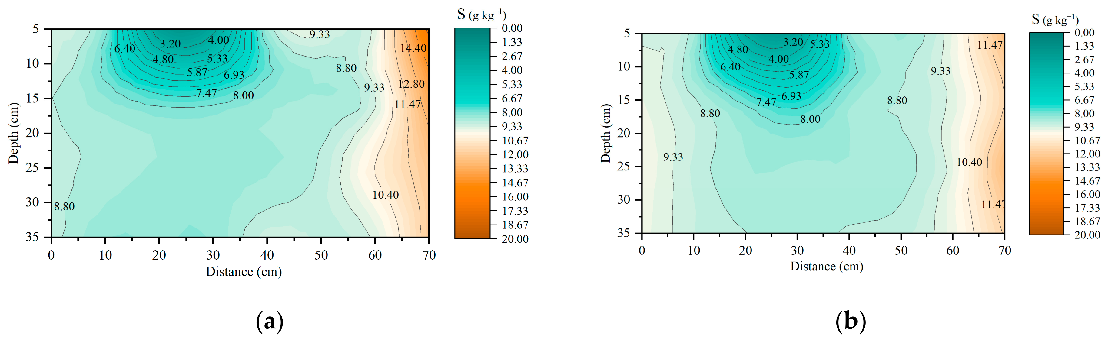
Figure 7. Simulated contours of soil salinity under W1, for (a) the middle of the first irrigation; (b) the middle of the third irrigation; (c) the middle of the fifth irrigation; (d) at the end of experiment.

Figure 7. Simulated contours of soil salinity under W1, for (a) the middle of the first irrigation; (b) the middle of the third irrigation; (c) the middle of the fifth irrigation; (d) at the end of experiment.

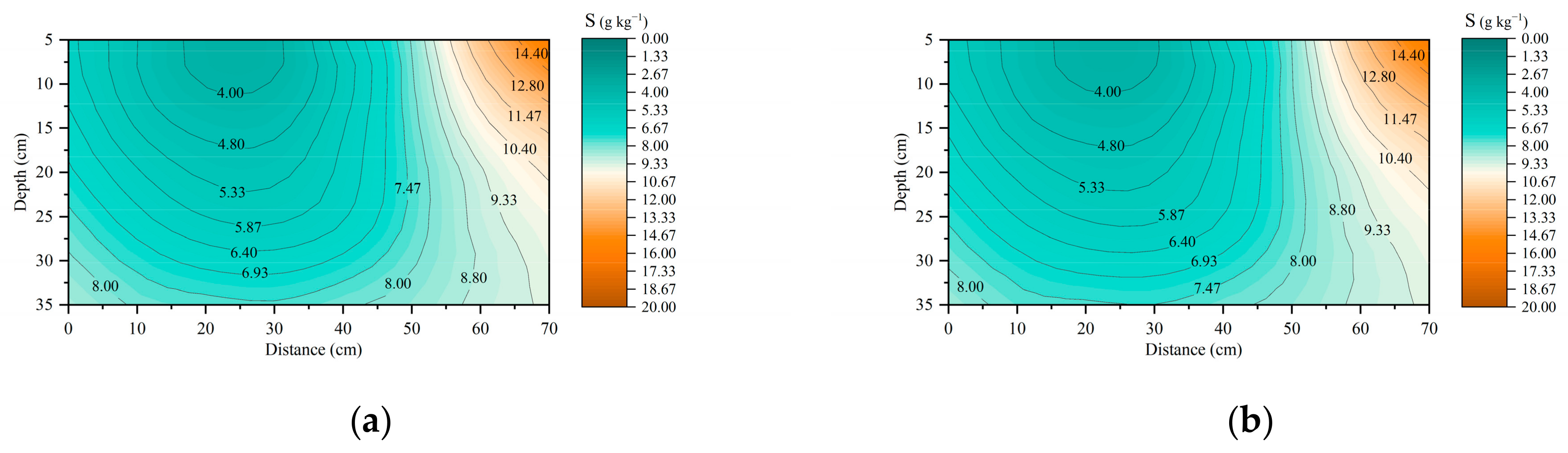
Figure 8. Simulated contours of soil salinity under W2, for (a) the middle of first irrigation; (b) the middle of third irrigation; (c) the middle of fifth irrigation; (d) at the end of experiment.

Figure 8. Simulated contours of soil salinity under W2, for (a) the middle of first irrigation; (b) the middle of third irrigation; (c) the middle of fifth irrigation; (d) at the end of experiment.

Figure 9. Measured 2D distribution of soil salinity at the end of experiment: (a) Measured distribution under W1; (b) under W2.

Figure 9. Measured 2D distribution of soil salinity at the end of experiment: (a) Measured distribution under W1; (b) under W2.

Figure 10. Simulated 2D distribution of soil salinity with instantaneous equilibrium adsorption at the end of experiment: (a) Simulated distribution under W1; (b) under W2.

Figure 10. Simulated 2D distribution of soil salinity with instantaneous equilibrium adsorption at the end of experiment: (a) Simulated distribution under W1; (b) under W2.

3.4. Heat Transport under Various Irrigation Treatments

The temperature distribution differences of the simulations and of the measurements taken in the middle of the first, third, and fifth irrigations and at the end of the experiment are shown in Figures S1–S4. Their ${\mathrm{R}}^2$ values were all larger than 0.6 and NRMSE values were all less than 17%. This indicates that the simulated temperature isotherm was consistent with the measurements, and that the model could reliably simulate the heat transport. However, an error was found to have occurred in the simulation. This was probably because the temperature boundary condition could not fully reflect the actual situation, especially on the soil surface. There the actual situation was too complex to be captured by simulation, due to the limitations in HYDRUS−2D’s boundary settings.

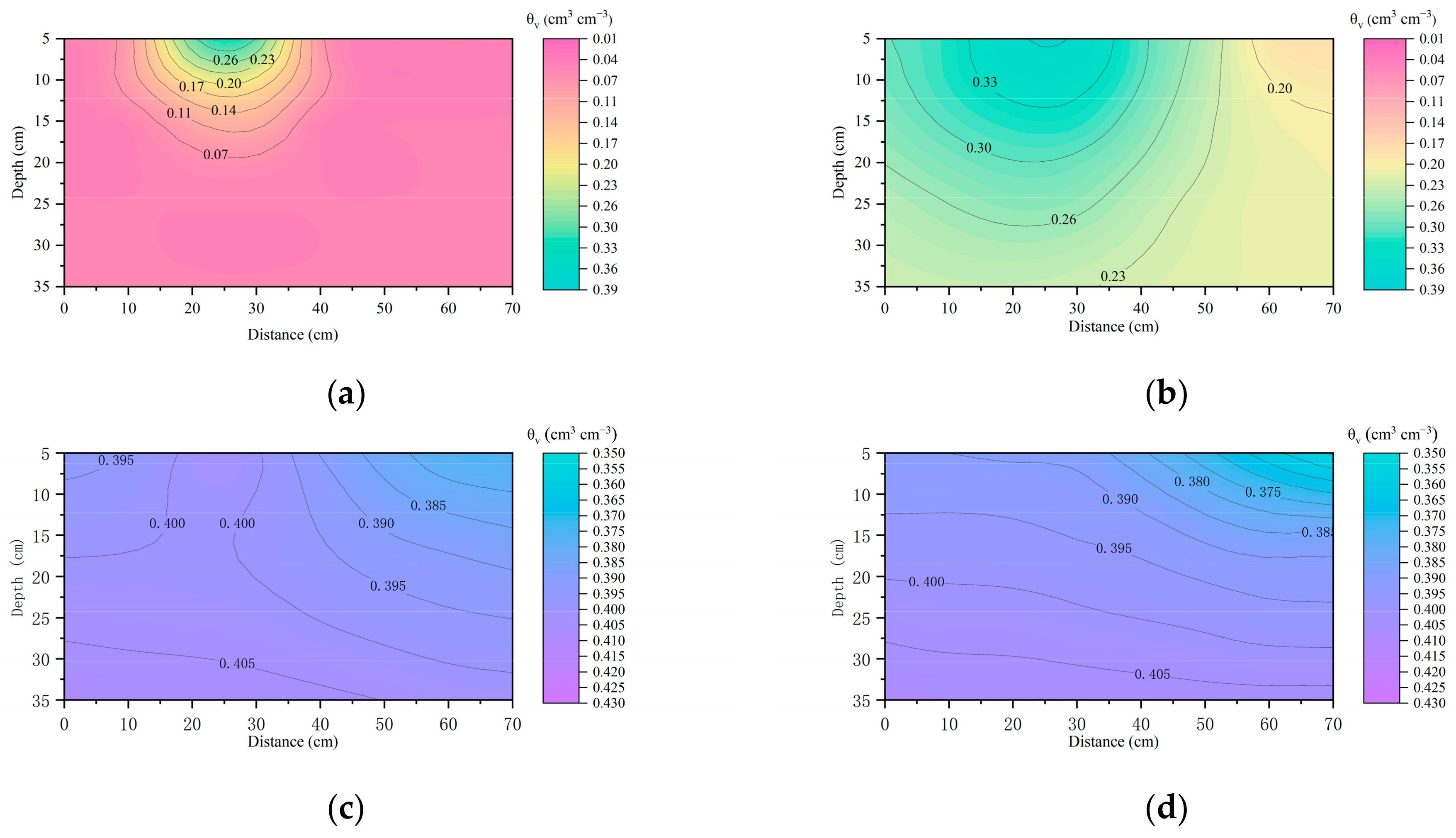
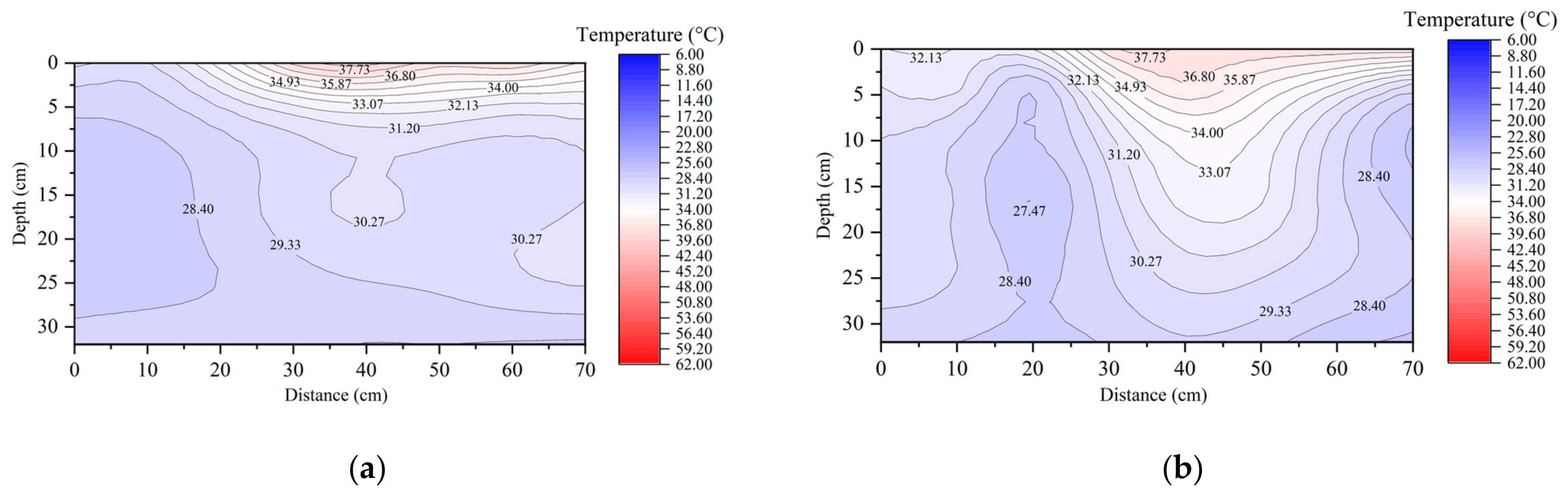
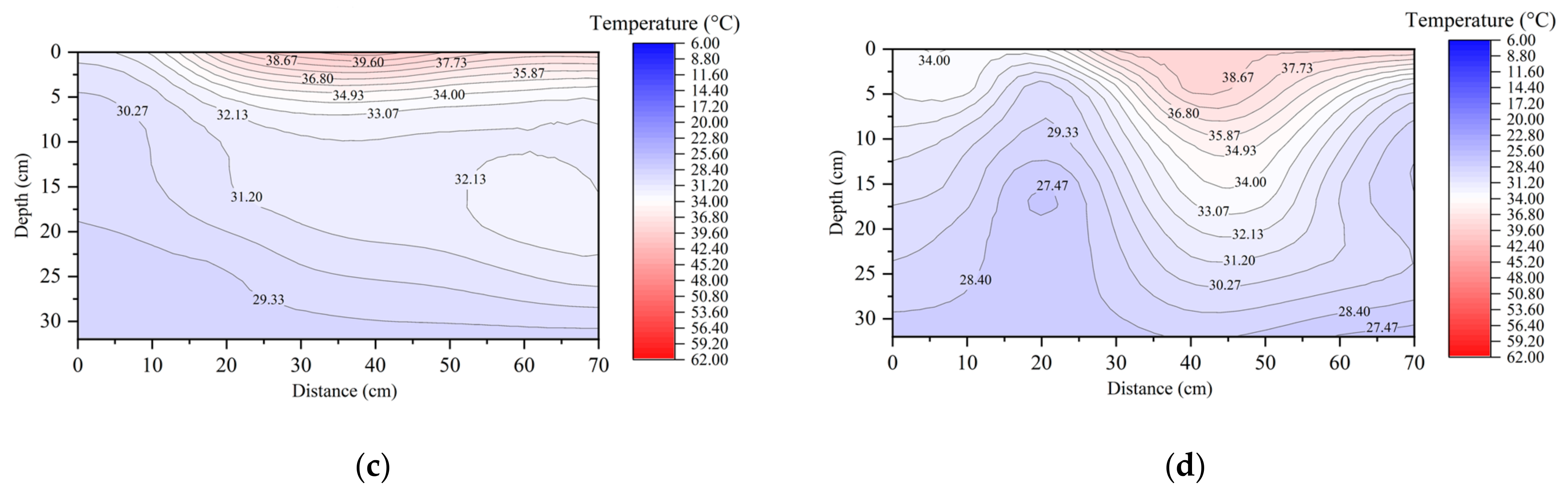
The average temperature was calculated to analyze the 2D temperature distribution during the entire experiment (Figure 11), to reflect effectively the heat condition over the time period. The temperature rise was more obvious at shallow depths, and decreased with the depth increase. At the soil surface there was also a difference in heat absorption between the un-mulched and mulched soil areas, due to the presence of mulch, consistent with previous findings [51]. In this study, the 2D soil profile was divided into three zones according to the position of mulch in relation to the dripper; i.e., the left area of mulched soil (ZL, 0–25 cm), the right area of mulched soil (ZR, 25–50 cm) and the un-mulched soil area (ZU, 50–70 cm). The ZR and ZU showed higher average temperatures (with higher temperature increases). Between the two, the average temperature in ZR was higher, which was because the mulch prevented the evaporation of water and reduced the latent heat consumption. In addition, the water in ZR migrated laterally to ZU, driven by evaporation, so the water content in these zones was lower than in ZL. The high specific heat capacity of water led to a slow temperature rise in ZL, and its average temperature was the lowest for the whole period. These results are consistent with previous film mulching studies, which showed that irrigation greatly affected soil temperature under mulch [49].

In order to explore the effects of mulch on heat transport in shallow areas where the soil temperature changed obviously, the daily mean measured temperature at 0–16 cm soil depth was considered. The shallow layer was divided into areas of mulched soil (0–50 cm) and un-mulched soil (50–70 cm). Maintaining uniformity in mind, Figure 12 presents the average temperatures of the un-mulched soil area and the mulched soil area for W2. The daily mean temperature of the whole mulched soil area (0–50 cm) at the same depth was always lower than that of the un-mulched soil area (50–70 cm). At greater soil depths, the temperature difference between the two zones gradually decreased. Consideration of the irrigation time reveals that the daily mean temperature rose after irrigation (for clarity, the data points when the temperature began to rise have been marked in the figure with triangle symbols (Δ) at the 0 cm mulched soil line). The specific heat capacity of water is higher than that of sandy loam [17]. Therefore, after being heated in the daytime, water continued to infiltrate and slowly released heat, which increased the soil temperature. This effect displayed a certain lag, because the temperature increase was behind the irrigation, which gradually decreased with an increase in the cumulative irrigation amount, similar to previous findings [49,54].

Figure 11. The 2D distribution diagram of average soil temperatures for the entire period: (a) Measured distribution under W1; (b) simulated distribution under W1; (c) measured distribution under W2; (d) simulated distribution under W2.

Figure 11. The 2D distribution diagram of average soil temperatures for the entire period: (a) Measured distribution under W1; (b) simulated distribution under W1; (c) measured distribution under W2; (d) simulated distribution under W2.

Figure 12. The daily mean temperature of soil at different depths and mulched conditions during the entire period for W2.

Figure 12. The daily mean temperature of soil at different depths and mulched conditions during the entire period for W2.

3.5. Discussion on the Coupling of Water, Salt, and Heat Transport

Previous analysis focused on the isolated aspects of water, salt, and heat. In fact, these three processes are coupled during transport, and are influenced by various factors (e.g., temporal, spatial, and water conditions) [28,53], which can be analyzed from four perspectives, i.e., spatial distribution, mechanism, time evolution, and treatment differences.

Previous indoor tank and field experiments using soil have investigated salt transport and the wetting front, and explored leaching efficiency in the root zone under different agricultural conditions [27,29,50]. For example, Chen et al. [29] conducted an indoor soil tank experiment, finding that horizontal tillage could increase the water storage capacity of soil underneath mulch and reduce soil salinization in the shallow soil layer. However, their study ignored the initial salt salinity in the bare soil area without horizontal tillage, which resulted in significant spatial differences. In terms of spatial difference, it was confirmed that the difference in hydrothermal conditions resulting from mulch led to differences in water, salt, and heat transport between mulched and un-mulched soil areas [23,24,25]; the differences in water and salt transport were the most significant. Differences in water and salt distribution were obvious in both the horizontal and the vertical directions of the soil profile. Meanwhile, the differences in heat distribution were more obvious in the shallow soil, which was consistent with the above results and previous findings [49].

In terms of the mechanism, the transport of water, salt, and heat influenced one another. The heat difference was a key factor that affected initial water and salt transport [55]. In the late irrigation period, salt crust in the un-mulched soil area blocked the water evaporation channel and intensified local heat accumulation [51]. Meantime, the differences in water and salt transport further influenced heat transport [56], jointly forming the specific 2D spatial distribution of water, salt, and heat.

From the perspective of time evolution, the two distinct salt zones (the salt accumulation area and the desalination area) were gradually formed under partially mulched conditions with drip irrigation, as clearly depicted by experiment and simulation.

From the perspective of different drip-irrigation intensities, under conditions of the same total irrigation amount, low levels of drip irrigation were observed to better reduce the salt in the root zone, while salt accumulation in the corresponding un-mulched soil area was more serious.

3.6. Simulation Scenarios

For the purpose of finding the optimum irrigation schedule to control salinity under partially mulched conditions, scenario simulations were conducted with various drip-irrigation schedules. The scenario design was similar to the above simulation, except that the bottom boundary was modified to a seepage boundary, which better reflected actual field conditions. The durations of the scenario simulations were 30 days, and the dates of drip irrigation were the same as in Table 1, with a total of 10 occurrences. Each drip irrigation lasted from 10:00 to 20:00. The irrigation increment coefficient (Ivar) was defined to describe the drip irrigation water allocation, as shown in Equation (26):

$$Ivar = \frac{{IA}_{i+1} -{ IA}_i}{{IA}_1}$$

(26)

where ${IA}_i$ is the drip irrigation amount for the $i$-$\mathrm{th}$, $i$ is the number of drip irrigations and $i$ = $1, 2, 3\dots 10$.

Figure 13 shows the soil salinity in the root zone (with a width of 5 cm around the position of the dripper and a depth of 15 cm below the soil surface) and the un-mulched soil surface, at the end of 30 days, for different total irrigation amounts (20–30 L) and water allocations (with Ivar between −0.5 to 0.5). In the case of decreasing drip irrigation treatments, smaller Ivar led to an improved desalination effect in the root zone and more serious salt accumulation near the un-mulched soil surface. The simulations produced similar results to those obtained in the earlier decremental drip-irrigation experiments, where a lower drip irrigation intensity (W1) was attributed to higher desalination efficiency in root zones. For the incremental drip irrigation treatments, the desalination effect and salt accumulation were more obvious with larger Ivar. In short, higher irrigation in the early stages led to rapid lateral migration of water and insufficient leaching of soil in the later stages, whereas higher irrigation in later stages effectively enhanced the short-term leaching effect. This was essentially consistent with a previous study of improving root-zone leaching efficiency by increasing the amount of drip irrigation [28]. Comparing the two sub-figures, suitable irrigation treatments can be identified to ensure the effective desalination of the root zone and the acceptable surface salinity of the un-mulched soil. As shown in Figure 13, the appropriate irrigation treatments between the two red contour lines formed the ideal desalination root zone (with soil salinity less than 0.6%) as well as identifying acceptable un-mulched soil surface salt conditions (with soil salinity less than 1.5%).

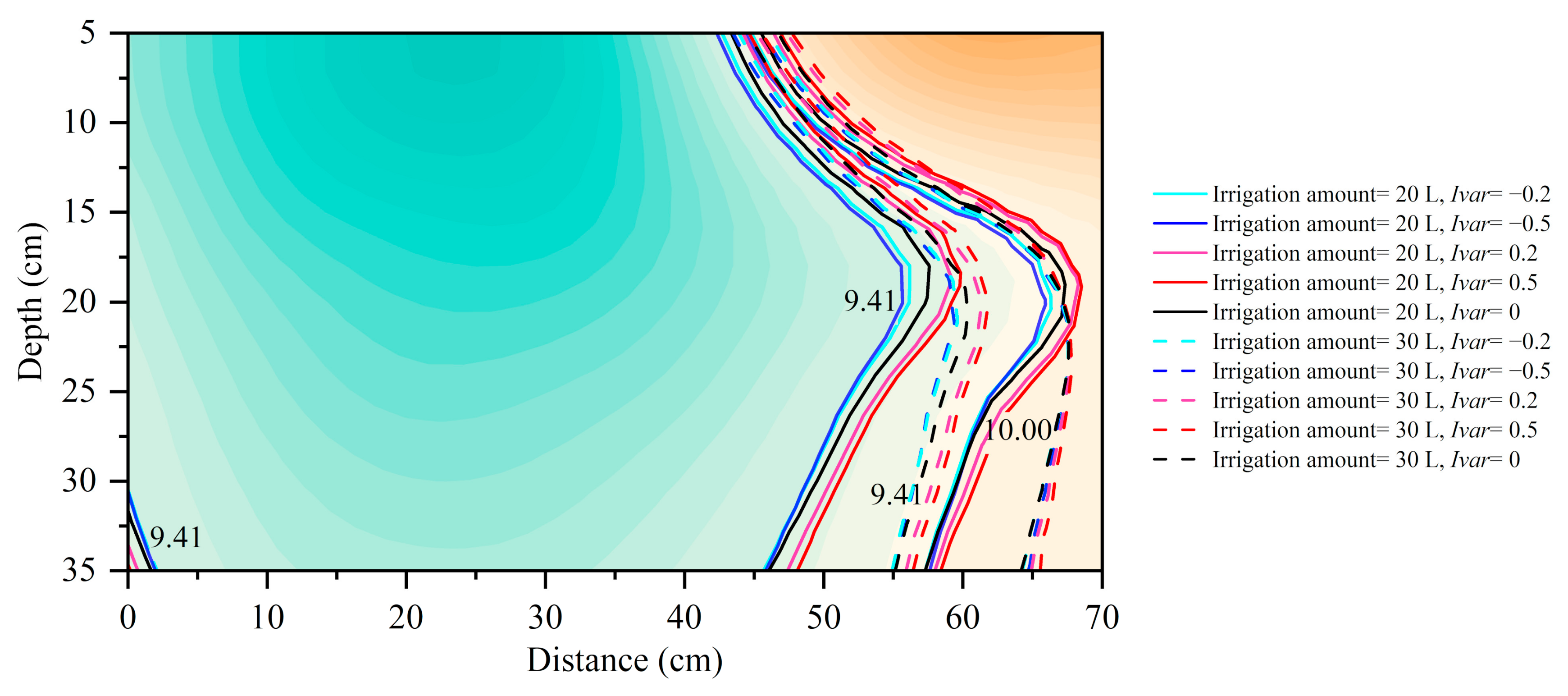
Figure 14 shows the 2D distribution of salt at the end of irrigation under different total irrigation amounts, along with the Ivar. The contour lines of 9.41 ${\mathrm{g} \mathrm{kg}}^{-1}$ and 10 ${\mathrm{g} \mathrm{kg}}^{-1}$ represent the boundary of the desalination zone and the soil salinity of 1%, respectively. First, the increase in the total irrigation amount obviously caused more lateral salt accumulation in the un-mulched soil area, where the soil salinity was greater than 1%. According to the scenario simulations, the position of the boundary between the desalination zone and the salt accumulation zone at 20 cm depth was relatively stable under different drip-irrigation treatments, whereas it was greatly influenced by the total irrigation amount in the deep soil layer. The increase in the total irrigation amount tended to leach salt to deeper depths, with the desalination boundary expanding accordingly. In the shallow un-mulched soil zone below 20 cm depth, salt accumulated due to evaporation, so the change in the desalination boundary was small. Moreover, the salt tended to migrate laterally instead of downwards, with alternate action of irrigation and evaporation. In a study of the salt migration law for cotton fields under partially mulched drip irrigation in arid areas, soil salt accumulated slowly in the vertical direction [5]. This is consistent with previous results, where higher drip-irrigation intensity in the later stages of incremental irrigation led to a better lateral desalination effect [33]. Therefore, under the same total amount of irrigation, managers can adopt incremental drip irrigation to achieve a better desalination effect in the root zone. The accompanying problem was higher salt accumulation in the un-mulched soil zone, and to control salt in the un-mulched soil zone, decremental drip-irrigation treatment was more appropriate.

Figure 13. Soil salinity under different total irrigation amounts, with Ivar, at the end of scenario. (a) Soil salinity in the root zone; (b) soil salinity in the un-mulched soil surface.

Figure 13. Soil salinity under different total irrigation amounts, with Ivar, at the end of scenario. (a) Soil salinity in the root zone; (b) soil salinity in the un-mulched soil surface.

Figure 14. The 2D distribution of soil salinity at the end of scenario under different total irrigation amounts, and Ivar, for simulations.

Figure 14. The 2D distribution of soil salinity at the end of scenario under different total irrigation amounts, and Ivar, for simulations.

4. Conclusions

In this study, two soil tank experiments were conducted, together with construction of a HYDRUS-2D model, to investigate the soil water, salt, and heat dynamics under partially mulched conditions with drip irrigation, in the sandy loam of southern Xinjiang. The main conclusions are as follows:

(1)

The HYDRUS-2D model compared reasonably well with the measured data, demonstrating that it can reflect differences in water, salt, and heat migration in the vertical and lateral directions. For solute transport, compared with instantaneous equilibrium adsorption, kinetic adsorption could better reflect the characteristics of solute transport in this experiment.

(2)

Under partially mulched drip irrigation, a significant difference was found in the migration of water, salt, and heat between the mulched and the un-mulched soil area. The un-mulched soil area was drier than the mulched soil area, and it also had higher soil salinity level and higher temperature rise with radiation.

(3)

For different irrigation intensities with the same total irrigation amount, lower intensity drip irrigation showed smaller spatial distribution difference for water, and larger spatial distribution differences in salinity and heat at the end of the process. Such treatment can lead to effective desalination in the mulched area; more serious salt accumulation was restricted to the un-mulched soil.

(4)

Scenario simulations showed that the total quantity of drip irrigation had an obvious effect on the desalination boundary in the deep soil layer. Drip irrigations with appropriate incremental intensity could improve salt leaching in the root zone, as more water migrates laterally.

References

- FAO. Land and Plant Nutrition Management Service; FAO: Rome, Italy, 2008; Available online: http://www.fao.org/ag/agl/agll/spush/ (accessed on 16 April 2021).
- Chen, W.; Hou, Z.; Wu, L.; Liang, Y.; Wei, C. Evaluating salinity distribution in soil irrigated with saline water in arid regions of northwest China. Agric. Water Manag. 2010, 97, 2001–2008. [Google Scholar] [CrossRef]
- Mai, W.X.; Tian, C.Y.; Li, C.J. Soil salinity dynamics under drip irrigation and mulch film and their effects on cotton root length. Commun. Soil Sci. Plant Anal. 2013, 44, 1489–1502. [Google Scholar] [CrossRef]
- Mu, H.; Hudan, T.; Su, L.; Mahemujiang, A.; Wang, Y.; Zhang, J. Salt transfer law for cotton field with drip irrigation under mulch in arid region. Trans. Chin. Soc. Agric. Eng. 2011, 27, 18–22. [Google Scholar] [CrossRef]
- Zhao, Y.; Mao, X.; Shukla, M.K.; Tian, F.; Hou, M.; Zhang, T.; Li, S. How does film mulching modify available energy, evapotranspiration, and crop coefficient during the seed—Maize growing season in northwest China? Agric. Water Manag. 2021, 245, 106666. [Google Scholar] [CrossRef]
- He, Q.; Li, S.; Kang, S.; Yang, H.; Qin, S. Simulation of water balance in a maize field under film–mulching drip irrigation. Agric. Water Manag. 2018, 210, 252–260. [Google Scholar] [CrossRef]
- Wang, J.; Tong, L.; Kang, S.; Li, F.; Zhang, X.; Ding, R.; Du, T.; Li, S. Flowering characteristics and yield of maize inbreds grown for hybrid seed production under deficit irrigation. Crop Sci. 2017, 57, 2238–2250. [Google Scholar] [CrossRef]
- Tian, D.; Zhang, Y.; Mu, Y.; Zhou, Y.; Zhang, C.; Liu, J. The effect of drip irrigation and drip fertigation on N2O and NO emissions, water saving and grain yields in a maize field in the North China Plain. Sci. Total Environ. 2017, 575, 1034–1040. [Google Scholar] [CrossRef]
- Cook, H.F.; Valdes, G.S.B.; Lee, H.C. Mulch effects on rainfall interception, soil physical characteristics and temperature under Zea mays L. Soil Tillage Res. 2006, 91, 227–235. [Google Scholar] [CrossRef]
- Ghosh, P.K.; Dayal, D.; Bandyopadhyay, K.K.; Mohanty, M. Evaluation of straw and polythene mulch for enhancing productivity of irrigated summer groundnut. Field Crops Res. 2006, 99, 76–86. [Google Scholar] [CrossRef]
- Ayars, J.E.; Phene, C.J.; Hutmacher, R.B.; Davis, K.R.; Schoneman, R.A.; Vail, S.S.; Mead, R.M. Subsurface drip irrigation of row crops: A review of 15 years of research at the water management research laboratory. Agric. Water Manag. 1999, 42, 1–27. [Google Scholar] [CrossRef]
- Yohannes, F.; Tadesse, T. Effect of drip and furrow irrigation and plant spacing on yield of tomato at dire dawa, Ethiopia. Agric. Water Manag. 1998, 35, 201–207. [Google Scholar] [CrossRef]
- Shao, G.; Cai, H.; Wu, L.; Zhang, Z. Prospect for the development of field drip irrigation under mulch in Xinjiang. Agric. Res. Arid Areas 2001, 19, 122–127. [Google Scholar] [CrossRef]
- Yang, P.; Dong, X.; Wei, G.; Ma, L.; Liu, L. Characteristics of salt deposition under drip irrigation beneath plastic film in arid area. Chin. J. Soil Sci. 2011, 42, 4. [Google Scholar] [CrossRef]
- Wang, Z.; Fan, B.; Guo, L. Soil salinization after long-term mulched drip irrigation poses a potential risk to agricultural sustainability. Eur. J. Soil Sci. 2011, 70, 20–24. [Google Scholar] [CrossRef]
- Li, Y.; Wang, W.Y.; Wang, Q.J. Application of drip irrigation technology under membrane in water-saving and salt-controlling irrigation in arid and semi-arid regions. J. Irrig. Drain. 2001, 20, 5. [Google Scholar] [CrossRef]
- Wang, J.; Gong, S.; Xu, D.; Juan, S.; Mu, J. Numerical simulations and validation of water flow and heat transport in a subsurface drip irrigation system using HYDRUS-2D. Irrig. Drain. 2013, 62, 97–106. [Google Scholar] [CrossRef]
- Selim, T.; Berndtson, R.; Persson, M. Simulation of soil water and salinity distribution under surface drip irrigation. Irrig. Drain. 2013, 62, 352–362. [Google Scholar] [CrossRef]
- Zapata-Sierra, A.J.; Roldán-Cañas, J.; Reyes-Requena, R.; Moreno-Pérez, M.F. Study of the Wet Bulb in Stratified Soils (Sand-Covered Soil) in Intensive Greenhouse Agriculture under Drip Irrigation by Calibrating the Hydrus-3D Model. Water 2021, 13, 600. [Google Scholar] [CrossRef]
- Shan, Y.; Wang, Q. Simulation of salinity distribution in the overlap zone with double-point-source drip irrigation using Hydrus-3D. Aust. J. Crop Sci. 2012, 6, 238–247. [Google Scholar]
- Zhao, Y.; Mao, X.; Shukla, M.K. A modified swap model for soil water and heat dynamics and seed—Maize growth under film mulching. Agric. For. Meteorol. 2020, 292–293, 108127. [Google Scholar] [CrossRef]
- Qi, Z.; Hao, F.; Ying, Z.; Zhang, T.; Zhang, A. Spatial distribution and simulation of soil moisture and salinity under mulched drip irrigation combined with tillage in an arid saline irrigation district, northwest China. Agric. Water Manag. 2018, 201, 219–231. [Google Scholar] [CrossRef]
- Bristow, K.L.; Horton, R. Modeling the impact of partial surface mulch on soil heat and water flow. Theor. Appl. Climatol. 1996, 54, 85–98. [Google Scholar] [CrossRef]
- Graefe, J. Simulation of soil heating in ridges partly covered with plastic mulch, part I: Energy balance model. Biosyst. Eng. 2005, 92, 391–407. [Google Scholar] [CrossRef]
- Graefe, J.; Schmidt, S.; Heissner, A. Simulation of soil heating in ridges partly covered with plastic mulch, part II: Model calibration and validation. Biosyst. Eng. 2005, 92, 495–512. [Google Scholar] [CrossRef]
- Zeng, W.Z.; Chi, X.; Wu, J.W.; Huang, J.S. Soil salt leaching under different irrigation regimes: HYDRUS-1D modelling and analysis. J. Arid Land 2014, 6, 44–58. [Google Scholar] [CrossRef]
- Chen, L.; Feng, Q.; Li, F.; Li, C. A bidirectional model for simulating soil water flow and salt transport under mulched drip irrigation with saline water. Agric. Water Manag. 2014, 146, 24–33. [Google Scholar] [CrossRef]
- Ning, S.; Zhou, B.; Shi, J.; Wang, Q. Soil water/salt balance and water productivity of typical irrigation schedules for cotton under film mulched drip irrigation in northern Xinjiang. Agric. Water Manag. 2021, 245, 106651. [Google Scholar] [CrossRef]
- Chen, W.; Li, M.; Qin, W.; Xu, Y.; Nie, J.; Liang, M. Effect of horizontal tillage measures regulatory on soil water and salt distribution under mulched drip irrigation. Trans. Chin. Soc. Agric. Mach. 2020, 51, 276–286. [Google Scholar] [CrossRef]
- Rehemui; Hudan, T.; Mahemut, A.; Zhao, J.H.; Alipujiang, A. Study on the numerical simulation of soil water and salt transport under mulch drip irrigation. Xinjiang Agric. Sci. 2015, 52, 2136–2141. [Google Scholar]
- Šimůnek, J.; Sejna, M.; van Genuchten, M.T. The HYDRUS-2D Software Package for Simulating Two-Dimensional Movement of Water, Heat, and Multiple Solutes in Variable Saturated Media Version 2.0.1GWMCTPS-53; International Ground Water Modeling Center, Colorado School of Mines: Golden, CO, USA, 1999; Available online: https://www.pc-progress.com/Downloads/Pgm_Hydrus2D/HYDRUS2D.PDF (accessed on 10 January 2022).
- Šimůnek, J.; Jacques, D.; Hopmans, J.W.; Inoue, M.; Flury, M.; van Genuchten, M.T. Solute transport during variably saturated flow-inverse methods. In Methods of Soil Analysis: Part 1, Physical Methods, 1st ed.; Dane, J.H., Topp, G.C., Eds.; Soil Science Society of America Journal: Madison, WI, USA, 2002; pp. 1435–1449. [Google Scholar] [CrossRef]
- Wang, Q.; Wang, W.; Lü, D.Q.; Wang, Z.R.; Zhang, J.F. Water and salt transport features for salt-effected soil through drip irrigation under film. Trans. Chin. Soc. Agric. Eng. 2000, 16, 54–57. [Google Scholar] [CrossRef]
- Yao, B.; Li, G.; Ye, H.; Li, F. Characteristics of spatial and temporal changes in soil salt content in cotton fields under mulched drip irrigation in arid oasis regions. Trans. Chin. Soc. Agric. Mach. 2016, 47, 11. [Google Scholar] [CrossRef]
- Kandelous, M.M.; Šimůnek, J. Numerical simulations of water movement in a subsurface drip irrigation system under field and laboratory conditions using HYDRUS-2D. Agric. Water Manag. 2010, 97, 1070–1076. [Google Scholar] [CrossRef]
- Van Genuchten, M.T. A closed-form equation for predicting the hydraulic conductivity of unsaturated soils. Soil Sci. Soc. Am. J. 1980, 44, 892–898. [Google Scholar] [CrossRef]
- Ippisch, O.; Vogel, H.J.; Bastian, P. Validity limits for the van genuchten-mualem model and implications for parameter estimation and numerical simulation. Adv. Water Resour. 2006, 29, 1780–1789. [Google Scholar] [CrossRef]
- Šimůnek, J.; Huang, K.; Van Genuchten, M.T. The SWMS-3D Code for Simulating Water Flow and Solute Transport in Three-Dimensional Variably Saturated Media Version 1.0; Research Report No. 139; U.S. Salinity Laboratory, USDA, ARS: Riverside, CA, USA, 1995; p. 155. Available online: https://www.ars.usda.gov/arsuserfiles/20361500/pdf_pubs/P1477.pdf (accessed on 12 January 2022).
- Van Genuchten, M.T.; Wagenet, R.J. Two-site/two-region models for pesticide transport and degradation: Theoretical development and analytical solutions. Soil Sci. Soc. Am. J. 1989, 53, 1303–1310. [Google Scholar] [CrossRef]
- Toride, N. Flux-averaged concentrations for transport in soils having nonuniform initial solute distributions. Soil Sci. Soc. Am. J. 1993, 57, 1406–1409. [Google Scholar] [CrossRef]
- Sophocleous, M. Analysis of water and heat flow in unsaturated-saturated porous media. Water Resour. Res. 1979, 15, 1195–1206. [Google Scholar] [CrossRef]
- Šimůnek, J.; Suarez, D.L. Modeling of carbon dioxide transport and production in soil: 1. Model development. Water Resour. Res. 1993, 29, 487–497. [Google Scholar] [CrossRef]
- Chung, S.-O.; Horton, R. Soil heat and water flow with a partial surface mulch. Water Resour. Res. 1987, 23, 2175–2186. [Google Scholar] [CrossRef]
- Schaap, M.G.; Leij, F.J.; Van Genuchten, M.T. Rosetta: A computer program for estimating soil hydraulic parameters with hierarchical pedotransfer functions. J. Hydrol. 2001, 251, 163–176. [Google Scholar] [CrossRef]
- Wang, S.; Wang, Q.; Fan, J.; Wang, W. Soil thermal properties determination and prediction model comparison. Trans. Chin. Soc. Agric. Eng. 2012, 28, 78–84. [Google Scholar] [CrossRef]
- Pan, M.; Huang, Q.; Feng, R.; Hang, G. Estimation of hydraulic and thermal parameters in saturated layered porous media based on heat tracing method. J. Hydraul. Eng. 2017, 48, 10. [Google Scholar] [CrossRef]
- Hu, J.H.; Zhao, W.J.; Liu, G.Y.; Hu, J.Z. Numerical Simulation of the Influence of Water and Soil Temperature on Water and Heat Transfer of Sand Mulching Soil under Drip Irrigation. J. Soil Water Conserv. 2020, 34, 349–354. [Google Scholar] [CrossRef]
- Chen, S.; Mao, X.; Shukla, M.K. Evaluating the effects of layered soils on water flow, solute transport, and crop growth with a coupled agro-eco-hydrological model. J. Soils Sediments 2020, 20, 3442–3458. [Google Scholar] [CrossRef]
- Sun, G.; Qu, Z.; Du, B.; Ren, Z.; Liu, A. Water-heat-salt effects of mulched drip irrigation maize with different irrigation scheduling in hetao irrigation district. Trans. Chin. Soc. Agric. Eng. 2017, 33, 144–152. [Google Scholar] [CrossRef]
- Wang, Y.M.; Husan, T.; Yi, P.F.; Zhang, J.Z.; Wu, Z.G.; Xu, F.L. Research on the Moment of Water and Salinity for Drip Irrigation under the Film under Saline and Alkali Soils. China Rural Water Hydropower 2010, 10, 13–17. [Google Scholar]
- Nachshon, U.; Weisbrod, N.; Dragila, M.I.; Grader, A. Combined evaporation and salt precipitation in homogeneous and heterogeneous porous media. Water Resour. Res. 2011, 47, 980–990. [Google Scholar] [CrossRef]
- Wu, Z.D.; Wang, Q.J. Saline water infiltration with different initial moisture contents. Trans. Chin. Soc. Agric. Mach. 2010, 41, 53–58. Available online: http://www.j-csam.org/jcsam/ch/reader/view_abstract.aspx?flag=1&file_no=2010s11&journal_id=jcsam (accessed on 26 July 2022).
- Li, M.; Liu, H.; Zheng, X. Spatiotemporal variation for soil salinity of field land under long-term mulched drip irrigation. Trans. Chin. Soc. Agric. Eng. 2012, 28, 82–87. [Google Scholar] [CrossRef]
- Liu, Q.; Li, W.; Zhao, G.; Jia, Z.; An, W.; Wang, J.; Mu, M. Effects of gravel-sand mulching and irrigation on soil hydrothermal conditions and fruit yield in ecological jujube forests on degraded field. J. Agric. Resour. Environ. 2022. Available online: http://agri.ckcest.cn/topic/downloadFile/d71a6748-c6dc-4e48-b054-82fe7de8760e (accessed on 26 July 2022).
- Wen, W.; Lai, Y.; You, Z. Numerical modeling of water—Heat—Vapor—Salt transport in unsaturated soil under evaporation. Int. J. Heat Mass Transf. 2020, 159, 120114. [Google Scholar] [CrossRef]
- Noborio, K.; Mclnnes, K.J. Thermal conductivity of salt-affected soils. Soil Sci. Soc. Am. J. 1993, 57, 329–334. [Google Scholar] [CrossRef]
Figure 3.
The schematic diagram of the model and its water boundaries.