1. Introduction
Soil evaporation is an essential part of the water cycle, which must be quantified in order to estimate water budgets. Accurate estimates of evaporation are often critical in agriculture for the determination of crop water demand and the implementation of optimal irrigation schedules for arable fields [
1,
2]. Despite its importance, the estimation of evaporation is challenging, and is dependent upon many variables (e.g., precipitation, ambient temperature, soil substrate thermal conductivity, permeability, capillary pressure etc.), with the mechanics of evaporation being complex and multi-faceted in nature [
3]. As evaporation is a main agent of water loss from the soil, efficient and sustainable water resource management requires the accurate quantification of evaporation rates, especially in arid regions where water is scarce. A major challenge towards the measurement of evaporations rates in such regions is that the climatic parameters that govern evaporation and recharge are highly variable, with long periods of drought punctuated by intense bouts of precipitation for a few hours or days per annum.
Arid regions are characterized by low rainfall (less than 150 mm) and high annual potential evapotranspiration. The ratio between precipitation and potential evapotranspiration expresses the degree of aridity. This ratio varies between 0.03 and 0.2 in arid countries, as most of the rainfall evaporates back into the atmosphere (Lehmann et al., 2019).
Stroosnijder (1987) [
3] found that the actual evaporation rate equals the potential rate on rainy days, and then reduces significantly afterward due to the under-saturated nature of soils in semi-arid regions. This behavior is accentuated in arid regions, where rainfall is very low, resulting in even higher soil-drying rates.
Several experimental approaches for land surface evaporation rate estimation have been applied. For example, several studies have employed the use of micrometeorological systems, which directly or indirectly measure water vapor fluxes into the atmosphere at the ground surface level [
4]. Some approaches are based on the turbulence theory (the eddy covariance method) or deduced from the relationship between gradients of water vapor concentration, and vertical water vapor flux [
5,
6]. However, micrometeorological methods are expensive and use sensors which can measure rapid fluctuations in wind speed and humidity, often requiring regular calibration [
6]. Moreover, micrometeorological devices need to be installed in study areas characterized by an expansive upwind area and cannot generally be used within isolated locations.
Weighing lysimeters and soil physical methods represent another important set of evaporation measurement approaches. Such methods utilize the principle of soil water balance to determine evaporation. Soil physical methods consist of an in situ study of soil profile. By obtaining the gain terms (precipitation, irrigation, and capillary rise), the loss terms (drainage and runoff), and the change in soil water content, the rate of evaporation can be calculated. Rain gauges are used to quantify the gain by precipitation and irrigation. The capillary rise is assumed to be negligible as the water table is deep and has no influence in the in situ-studied soil profile. The determination of soil water content using this method requires a detailed measurement of soil moisture content over time. The soil moisture profile can be obtained using neutron probes or gamma ray scanners, which require a licensed operator, intensive work for installation, and high cost. Soil moisture profiles can be obtained using neutron probes or gamma-ray scanners, which usually require a licensed operator, complex installation, potential radiation exposure hazards, and high cost [
6,
7]. These practical limitations often prevent the use of soil physical methods for evaporation determination in many field areas.
Lysimeters measure changes in soil water storage and leakage, which directly enable the determination of evaporation and evapotranspiration. They consist of enclosed tanks filled with an undisturbed soil core and offer one of the few methods capable continuously measuring evaporation and percolation through soils [
8,
9,
10]. Such devices have been widely developed worldwide for evaporation studies over the last 80 years [
11,
12]. Advances in lysimeter hardware, data storage, and processing have facilitated the accurate determination of water mass balance, allowing the continuous and efficient monitoring of soil evaporation. One drawback of the lysimeters is that they are often expensive and require continuous maintenance. Lysimeters use either weighing or non-weighing configurations. Non-weighing lysimeters indirectly determine evaporation rates via volume balance, whereas weighing-based systems directly measure the amount of water loss or gain per unit time.
It is well recognized that the majority of the rainfall in arid areas is exchanged back into the atmosphere via evaporation or evapotranspiration. However, little is known about the actual measurements, as most studies cite values derived through indirect means. In this study, we showcase the direct measurement of soil moisture dynamics within arid regions through a case study from the State of Qatar. Whilst several studies in Qatar focused on potential evaporation estimates using proxy methods [
13,
14], the in situ physical measurement of evaporation remains unexplored. Bazaraa (1989) [
14] used various methods to calculate the potential evapotranspiration in Qatar, based on meteorological data from three locations across the country: Rodhat AI-Faras in the north, AI-Utoreyah in Qatar’s central portion, and Abu-Samara in the south-west of the country. Their results suggest that the potential evapotranspiration varies between 2.29 to 7.85 mm per day. These calculations were based on Blaney-Criddle, Thornthwaite, pan evaporation, and radiation methods, as well as Pen-man. Eccleston et al., (1981) [
13] used meteorological data from three stations in Qatar (Rodhat Al Faras, Decca, and Ahu Samra) to calculate open-water evaporation. They found that the daily evaporation varies between 2.5 mm/day during the winter months and 11.5 mm/day during the summer. Al-Ghobari (2000) [
15] compared the results of five methods for evapotranspiration in Saudi Arabia, with the estimated rates varying between 3 and 12 mm per day.
Though the direct quantification of evaporation is essential for water budget analyses, irrigation management, and the study of soil moisture dynamics, such measurements are generally rare, owing to the practical challenges related to their collation. This study uses data from field-weighing lysimeters to calculate the actual surface evaporation in calcareous soil within arid regions. In this work, we present one and a half years’ worth of time series data obtained from smart field lysimeters installed in unirrigated land using typical soil profiles from the northern part of the country. Data for the period between February 2018 and July 2019 are used to understand and analyze soil moisture fluctuation, temperature, matric potential, leakage, and evaporation.
2. Materials and Methods
2.1. The Study Area
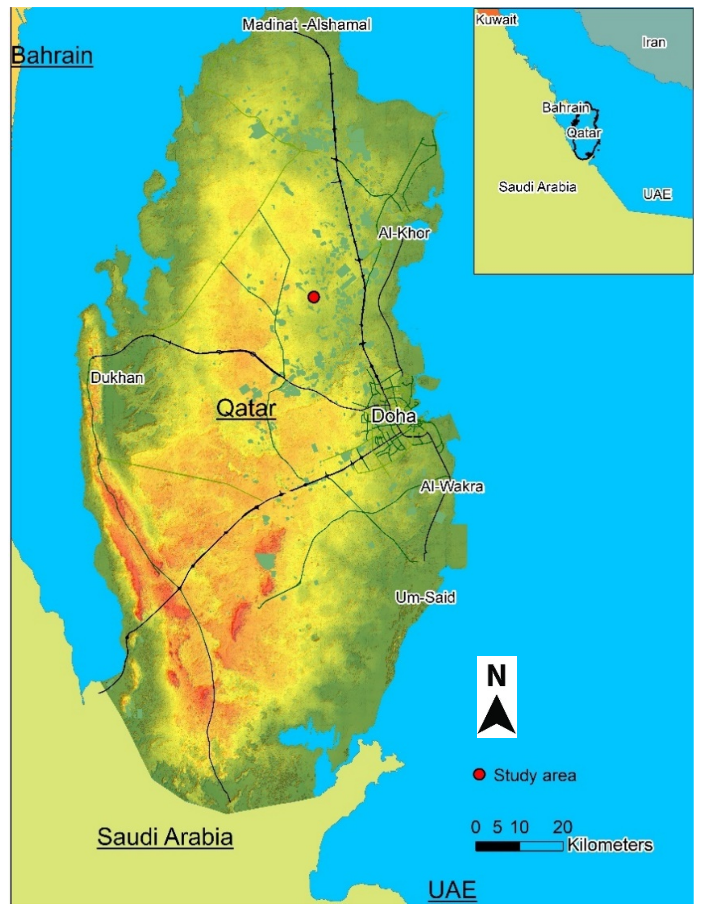
Qatar is located in the eastern part of the Arabian Peninsula (
Figure 1) and has an area of around 11,500 km
2. It is surrounded by the Arabian Gulf from all directions except the south, where it shares a land border with Saudi Arabia. The country is very arid due to low rainfall, and is characterized by relatively low relief, with a maximum height of 103 m above mean sea level at Qurain Abu al-Bawl. The topography is characterized by land depressions formed due to salt dissolution/collapse and karstification. Soil cover is generally very poor due to arid conditions and the lack of clastic input since the last glacial maximum, except for land depressions where loamy soil is accumulated by runoff.
The weather in Qatar can be broadly classified into two main seasons: a hot summer from May to October and winter from December to February, with transitional months in between. The average annual temperature is 27.0 °C, with an average annual rainfall of 80 mm per year, which can be highly variable over consecutive years (15, 5). Rainfall is very erratic and occurs between November and March [
16]. As the area of study is very arid, rainy days occur just a few times per annum, mostly as a result of thunder storms between September and April [
13].
Flash floods resulting from these thunderstorms account for much of the recharge potential in Qatar, whereby rainfall runoff accumulates in land depressions and eventually recharges the aquifer [
13,
17,
18]. Like other arid regions, Qatar is characterized by high-potential evapotranspiration rates.
Two smart field weighing lysimeters were installed using soil profiles from the Abu Thayla area (red dot on
Figure 1), which is typical of many land depressions in the country. The area is located at 25°31.9843′ N and 51°18.2824′ E, and it is a well-field area for Qatar General Electricity and Water Corporation (KAHRAMAA). Land depressions are very common in Qatar (locally known as roda) and likely form due to the dissolution of carbonate-evaporite sequences within the subsurface and subsurface slat collapse, especially in the southern part. Rainfall runoff transports loamy sediment into the land depressions, making them amendable to agriculture. Rainwater accumulates in the land depressions and eventually infiltrates through the soil column, contributing toward aquifer recharge. This area was selected because it anecdotally represents a typical recharge area and soil profile. The location is above a potable aquifer within the north of Qatar (northern aquifer) [
19,
20,
21].
2.2. Smart Field Lysimeters
Two lysimeters from Meter Environment Company (Meter Group) were installed in the field locations described above. These lysimeters had a depth of 60 cm and an inner diameter of 30 cm (model SFL-600). Two field boxes were connected to the lysimeters and a logger box was mounted nearby to collect data and send them through a file transfer protocol (FTP) server. Each lysimeter had six sensor ports: two each at depths of 5, 35, and 55 cm from the land surface. The cylinder was placed on a high-precision balance (PL-200), which measures the weight of the stainless cylinder with its contained soil column at one-minute intervals in order to monitor the localized water flux (i.e., an exchange with the atmosphere via precipitation and evaporation at the top, and with the lower soil by leakage at the bottom).
The two lysimeters contained undisturbed loamy soil, and the lower boundary was maintained at similar conditions to the surrounding field. The study area was not irrigated, meaning that measured evaporation and leakage reflected natural conditions. There was no vegetation cover in the area, except for seasonal desert plants and shrubs that grew after sporadic rainfall episodes and then died out during the summer.
The probes used in the lysimeters were (i) the ECH2O 5Te soil moisture sensor, which measured soil moisture, electric conductivity, and temperature, and (ii) the MPS-2 dielectric water potential sensor probes used for matric potential measurements.
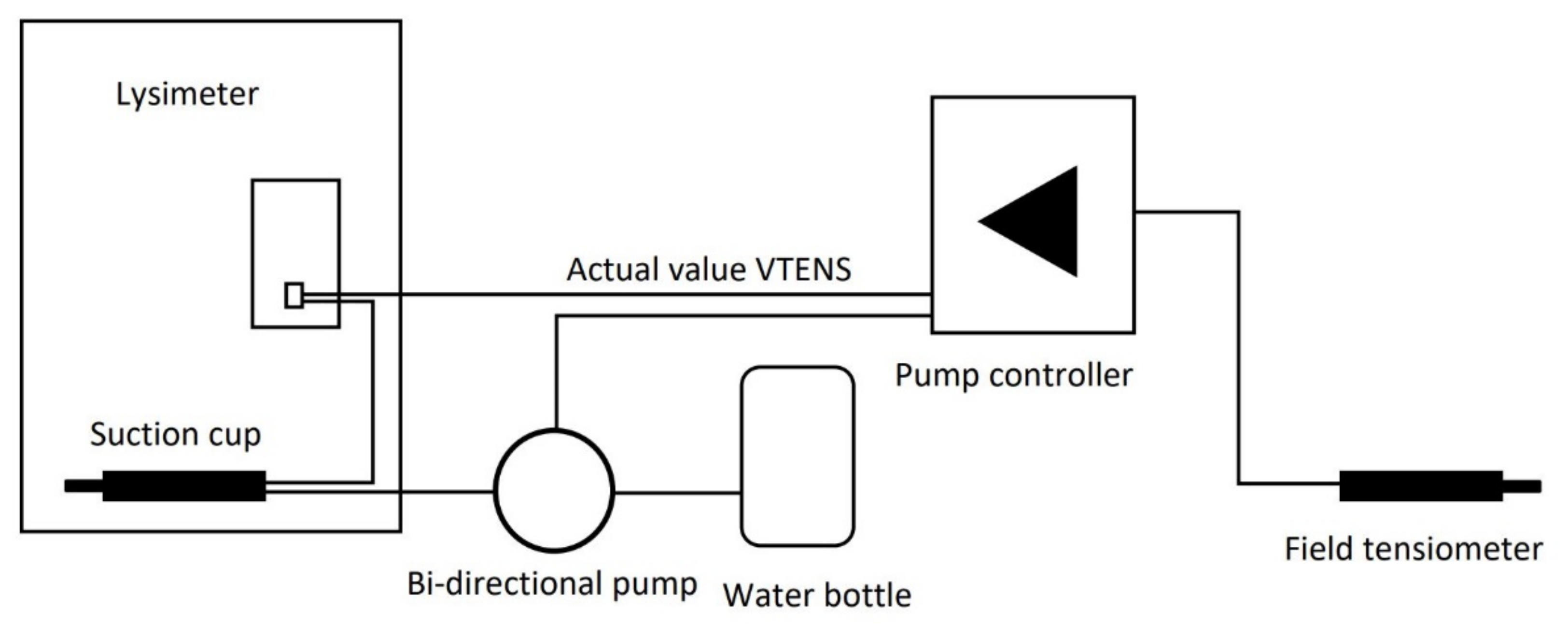
Figure 2 shows a schematic representation of how the lysimeter works. All probes were connected through a distribution box, which was directly mounted at the lysimeter. Further to this, a pressure sensor tested the value of the virtual tensiometer (VTENS), which represents the controlled boundary condition at the lowest part of the lysimeter cylinder. The VTENS provided a 4th matrix potential value just above the bottom of the cylinder. To maintain equivalent field conditions inside the cylinder, the smart field lysimeter used a feedback control by the means of a T8 reference tensiometer, which was placed into the soil close to the lysimeter. This feedback control represents the primary advantage of smart field lysimeters over conventional systems, as it enables soil humidity, water flux, and potential inside the lysimeter to be matched to ambient conditions. Both the lysimeter and the water bottles sat on separate scales which provided continuous readings. A continuous change in the VTENS value was automatically undertaken with the T8 reference tensiometer through a bi-directional pump that could pump water to or from a drainage water bottle located inside the field box (
Figure 2).
As shown in
Figure 2, each field box contained a drain water bottle placed on a balance and a system of bi-directional pumps. The whole system was connected to a data logger powered by a solar panel.
2.3. Lysimeter Data
Lysimeter data loggers were set up to collect data using two intervals: 1-min and 10-min increments. The 10-min increment data included the volumetric soil moisture [WC%], the soil temperature [T-deg C], the soil matric potential [MPS-KPa], and the electrical conductivity [EC-mS/cm], whereas the one-minute increment data included the lysimeter weight [LYW-kg], water storage tank weights [WWY-kg], and the pumping rate (i.e., for the lysimeter inlet and the lysimeter outlet). Lysimeters were installed in late February 2018, with data collection commencing shortly after. For this study, data analysis was carried out from 1 March 2018 to 31 July 2019, comprising a time series of more than 745,000 data points. This period encompasses more than a full hydrological year for the study area.
We pre-processed the lysimeter time series datasets to exclude points with anomalous or missing data. After cleaning operations, data analysis focused on days where rainfall was detected.
2.4. Lysimeters Calculations
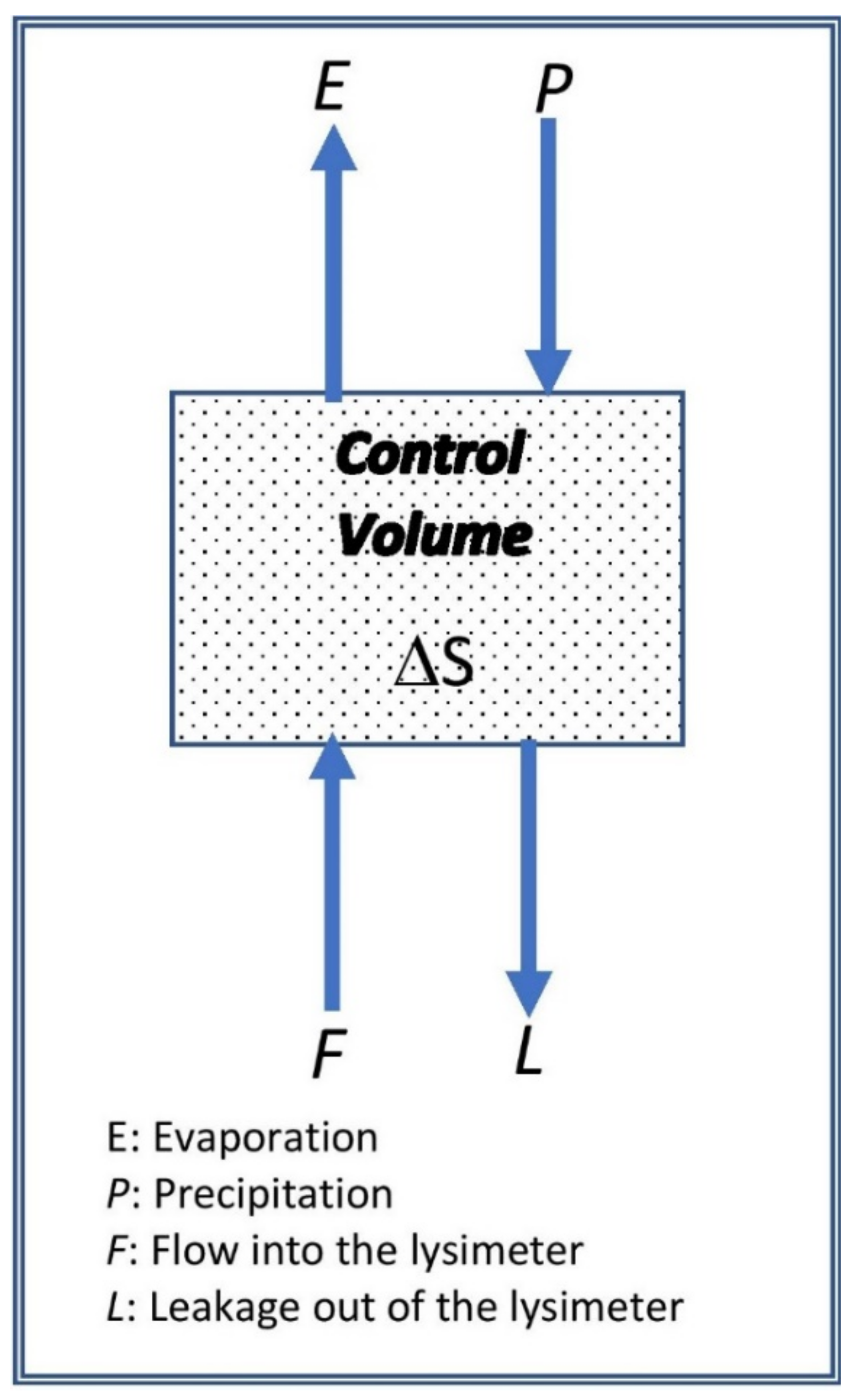
A schematic representation of a control volume representing the lysimeter is displayed in
Figure 3. Inflow into the lysimeter occurred through precipitation (P) and flow from the water tank (F). The latter is the component that mimics the field conditions by pumping water into the lysimeter through the T8 tensiometer. L is the outflow component of the T8 tensiometer, which is revealed via leakage out of the lysimeter. The last outflow component is evaporation (E). The difference between inflow and outflow equals the change in soil moisture content (ΔS), corresponding to the change in the lysimeter’s weight.
The field capacity (FC) and wilting point (WP) represent two important soil moisture thresholds. The field capacity is the amount of moisture that remains in the soil after all excess water has drained freely downward. For the soil type in this study, the FC was around 35%. The wilting point is the amount of moisture in the soil, below which plants are unable to uptake water. For the loamy soil in this study, the WP soil moisture varied between 10% and 15%. FC and WP are useful measures, particularly in the design of irrigation schemes. The ideal water content for plants should vary between FC and WP.
As precipitation infiltrates into the lysimeters, the soil moisture content increases until it reaches FC, after which leakage to the lower part of the lysimeter occurs. If the leakage rate is high enough, the water will enter the lysimeter’s leakage tank. The leakage rate can be calculated as the leakage volume in the tank divided by the surface area of the lysimeter. The surface area of the lysimeters used in this study was 0.0707 m
2. A one-kilogram increase in the leakage tank weight equals a one-liter volume of precipitation (assuming deionized water density) or 14.144 mm of rain. The leakage rate at a given time step n is:
where
Tw(
n) is the water tank weight at the time step
n. Similarly, the precipitation rate
P [mm] is the sum of the change in the lysimeter weight and the leakage water in the tank
where
Lw is the lysimeter weight. If there is no drained water, the precipitation equals the increase in the lysimeter weight.
Evaporation
E [mm] equals the difference between precipitation and the change in lysimeter weight plus changes in the leakage tank weight:
The change in the lysimeter weight represents an increase or decrease in the soil moisture. From Equations (1) and (2),
E can be written as:
where all weights are in kg. In dry seasons, no leakage occurs, and some water may transfer from the water tank into the lysimeter to mimic field conditions. In this case, the change in water tank weight will be negative. The leakage term L will be replaced by F, as shown in
Figure 3.
2.5. Unsaturated Flow Modelling
Modelling work was carried out to check the results of the lysimeter. Samples of undisturbed soil were collected from the field (i.e., the same location of the lysimeters) and various tests were carried out. This includes saturated hydraulic conductivity and soil moisture retention. The pressure plate experiment was carried out to determine soil moisture at saturation (
θs), the inflection point of the retention curve, and the residual soil moisture (
θr). These values were 0.41, 0.04, and 0.27, respectively. The saturated hydraulic conductivity was 1.48 cm/day. Van Genuchten (1980) [
23] described the water retention model as follows:
where
θ(
h) is the water content at matric potential
h,
α and
n parameters describing the shape of the water retention function, and
m = 1
− 1/
n.
Equation (5) can be used in conjunction with another equation describing the unsaturated hydraulic conductivity [
24]:
where
K(h) is the hydraulic conductivity at the matric potential
h,
Ks is the saturated hydraulic conductivity,
Se is the effective water content, and
l is a parameter describing the pore structure. The parameter m is described before. By obtaining the saturated hydraulic conductivity, as well as the saturated and residual moisture content, the parameters
n and
α can be obtained.
2.6. Hydrus 1D Model
Evaporation was simulated using Hydrus 1D software. Hydrus 1D can simulate water, heat, and solute flow in variably saturated media [
25]. The solution is based on the van Genuchten-Mualem model, as described in Equations (4) and (5). The flow in the variably saturated media is represented by Richard’s equation, ignoring the air phase and the thermal gradient:
where
h is the pressure head [L],
θ is the volumetric water content,
K is the unsaturated hydraulic conductivity,
S is the sink term, and
β is the angle between the flow and vertical access. The unsaturated hydraulic conductivity is given by:
where
Kr is the relative hydraulic conductivity as a function of head and location, and
Ks is the saturated hydraulic conductivity.
Table 1 lists the various parameters used in the Hydrus model.
2.7. Model Boundaries
The soil profile of the lysimeter is represented in the Hydrus model as the 1D profile, utilizing the soil moisture data at various depths within the profile. The upper boundary is the atmospheric conditions and the lower boundary is the free drainage. This allows water to move in either direction as the evaporation (upwards) or drainage (downwards). The model was run for summer months and winter months, with each run spanning 30 days.
2.8. Model Calibration
The van Genuchten parameters,
α and
n, were the calibrated parameters in this study. The initial values of these parameters were inputted based on soil analysis and literature values. To determine
α and
n, the time series of the soil moisture values from the field were fitted against the calculated values using the van Genuchten equation (Equation (5)). The fitting was based on the least square method. The least square analysis was implemented on an Excel spreadsheet, and the results were obtained when the objective function was minimized. The objective function was calculated by:
where
θm is the measured soil moisture in the field and
θcalc refers to the calculations from Equation (5) at the
n number of model nodes. To determine
α and
n, the measured values from the lab were fitted to the curve using the van Genuchten equation (Equation (5)). The fitting was based on least square, using an Excel spreadsheet [
26]. The results show that
α = 0.029 and
n = 1.4.
3. Results and Discussion
3.1. Temperature Fluctuation
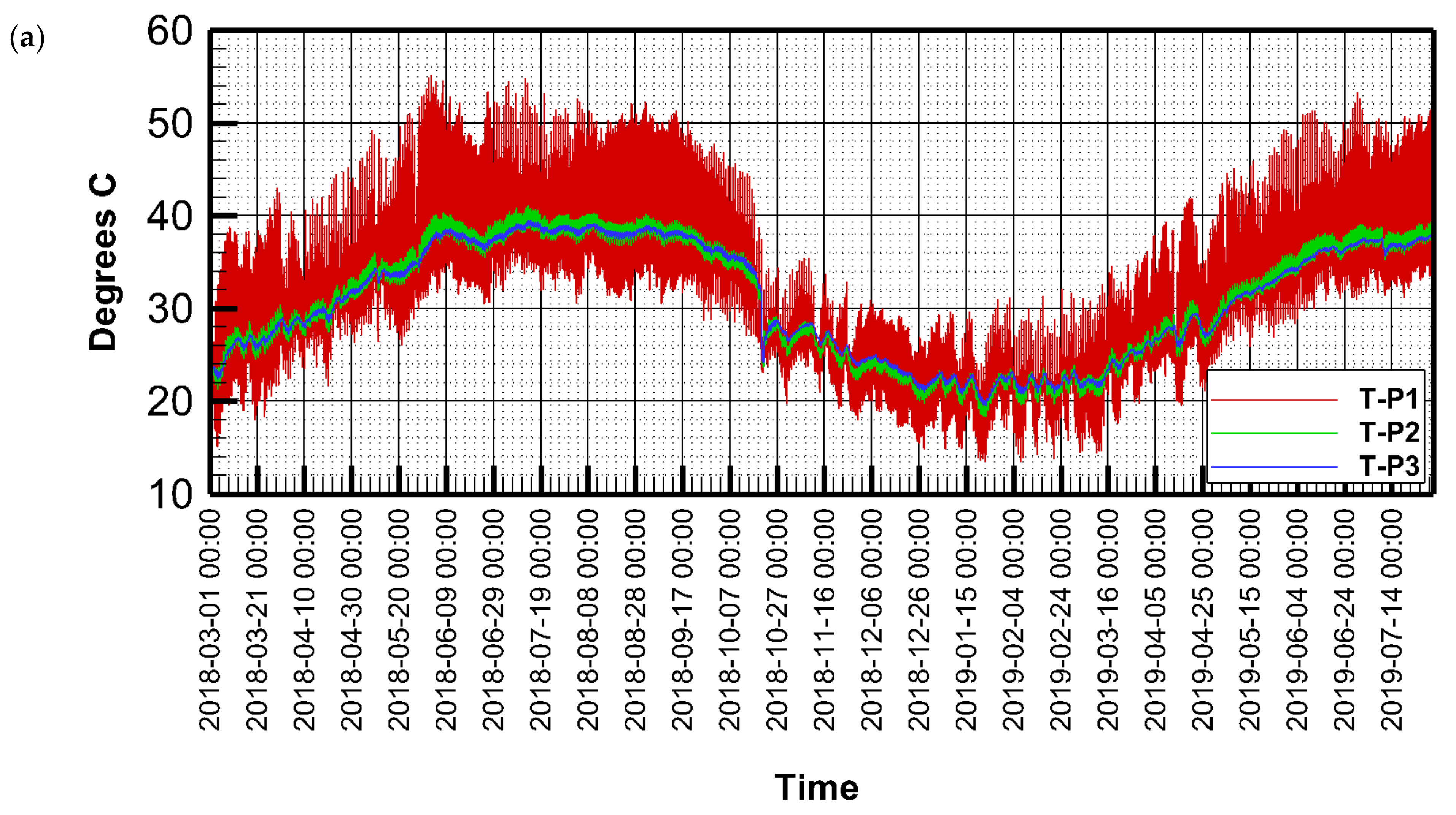
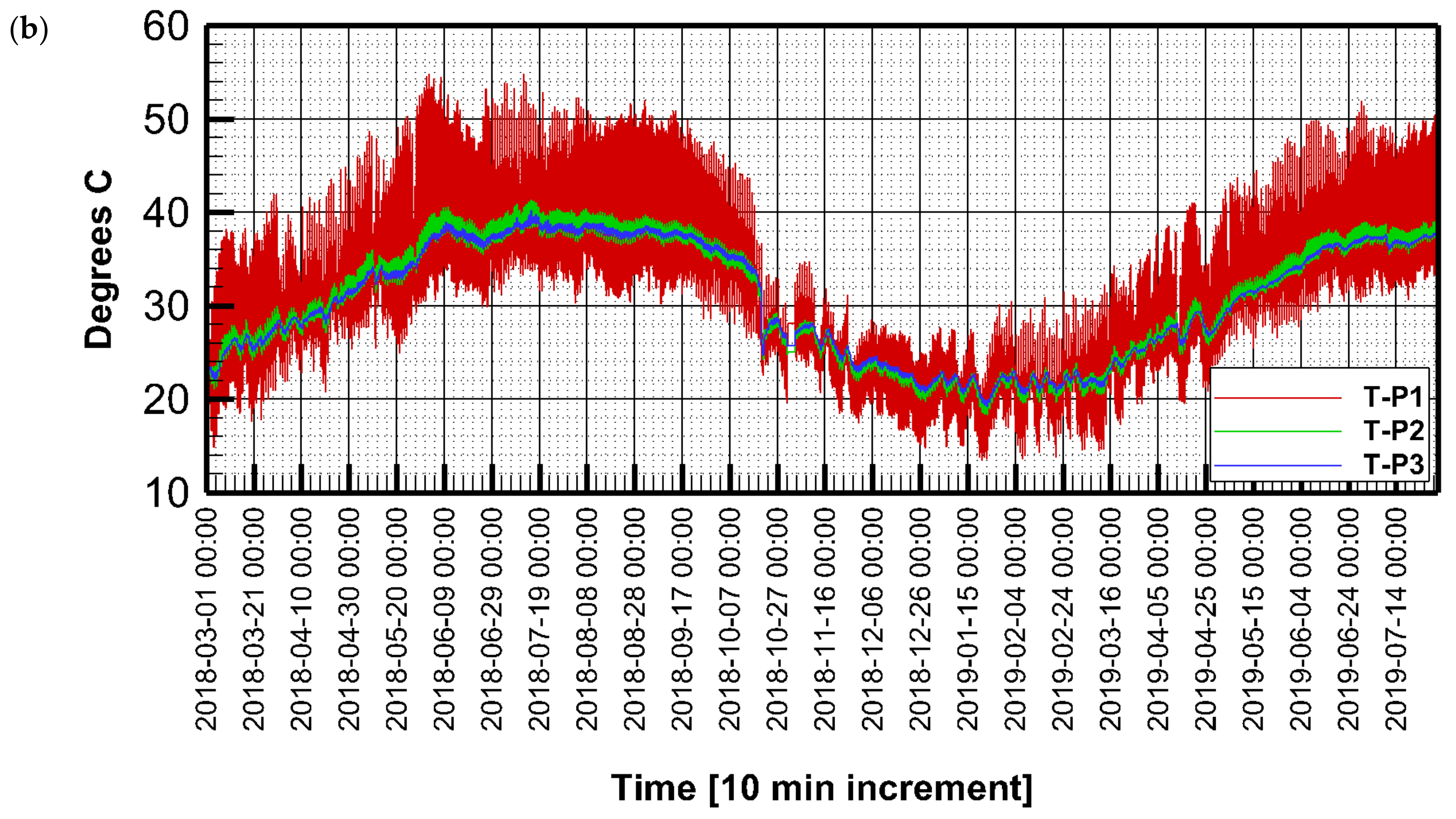
Three temperature probes in each lysimeter recorded the soil temperature every 10 min at depths of 5, 35, and 55 cm from the soil surface, designated as T-P1, T-P2, and T-P3, respectively.
Figure 4 shows fluctuations in temperature over the study period for both lysimeters 1 and 2.
The upper probe (T-P1) shows high fluctuation, as it is closer to the ambient air temperature, whereas temperatures at the lower probe were stable. The highest recorded temperature at the upper probe (T-P1) was 55.1 °C, which was recorded around noontime on the 2 June 2018, and 12 July 2018. The lowest recorded temperature at the upper probe was 13.4 °C, which was recorded in the early hours of the morning on the 23 January 2019 and the 7 February 2019. The minimum temperature at the probe T-P2 was 18.3 °C, which was recorded on 22 January 2019, and the maximum was 41.10 °C, which was recorded on the 13 July 2018. The minimum temperature at T-P3 was 19.40 °C, which was recorded on 23 of January, and the maximum temperature was 39.40 °C, which was recorded on 13 July 2018. Despite the high variability of temperature, the average values were 31.97 °C, 30.82 °C, and 30.78 °C for T-P1, T-P2, and T-P3, respectively.
3.2. Soil Moisture
Variations in soil moisture were mainly dependent upon rainfall and evaporation rates. Rainfall in Qatar was very erratic, with high variability from year to year. The total rainfall varied between 10 mm and 200 mm per annum, with a long-term average of around 80 mm. In terms of spatial distribution, received rainfall tended to decrease from north to south. Rainfall mainly occurred between the months of November and March [
13], but sometimes occurred outside this period (i.e., as early as September and as late as April). Various studies estimated annual groundwater recharge from rainfall, as summarized by [
18].
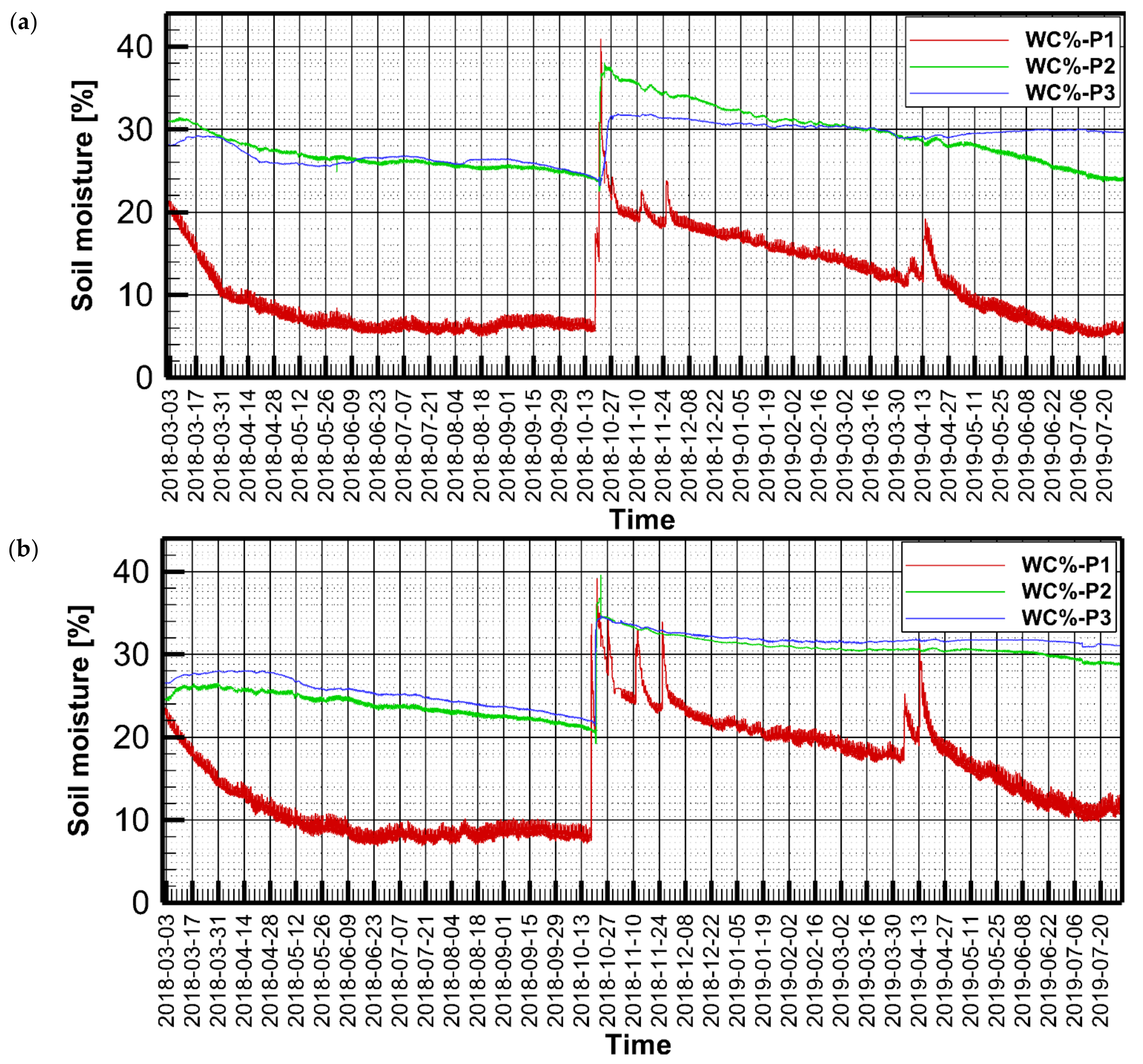
The volumetric soil moisture values (in %) are presented in
Figure 5 for lysimeters 1 and 2. Several rainfall events occurred in October and April 2019, which appear as spikes in the soil moisture time series of the shallow probe (P1), whereas the deeper probes show a slower response to rainfall.
Soil moisture varied between 6% and 35%. While the moisture content at the upper probe showed high variability due to proximity to the land surface, the lower ones were less variable. In general, the maximum soil moisture was reached during wintertime, and then started to gradually decrease, reaching the lowest level by the end of the summer (i.e., during August). While the soil profiles in both lysimeters came from the same area (around 100 m apart), they showed high variability between one another.
3.3. Soil Moisture Dynamics
3.3.1. November 2018
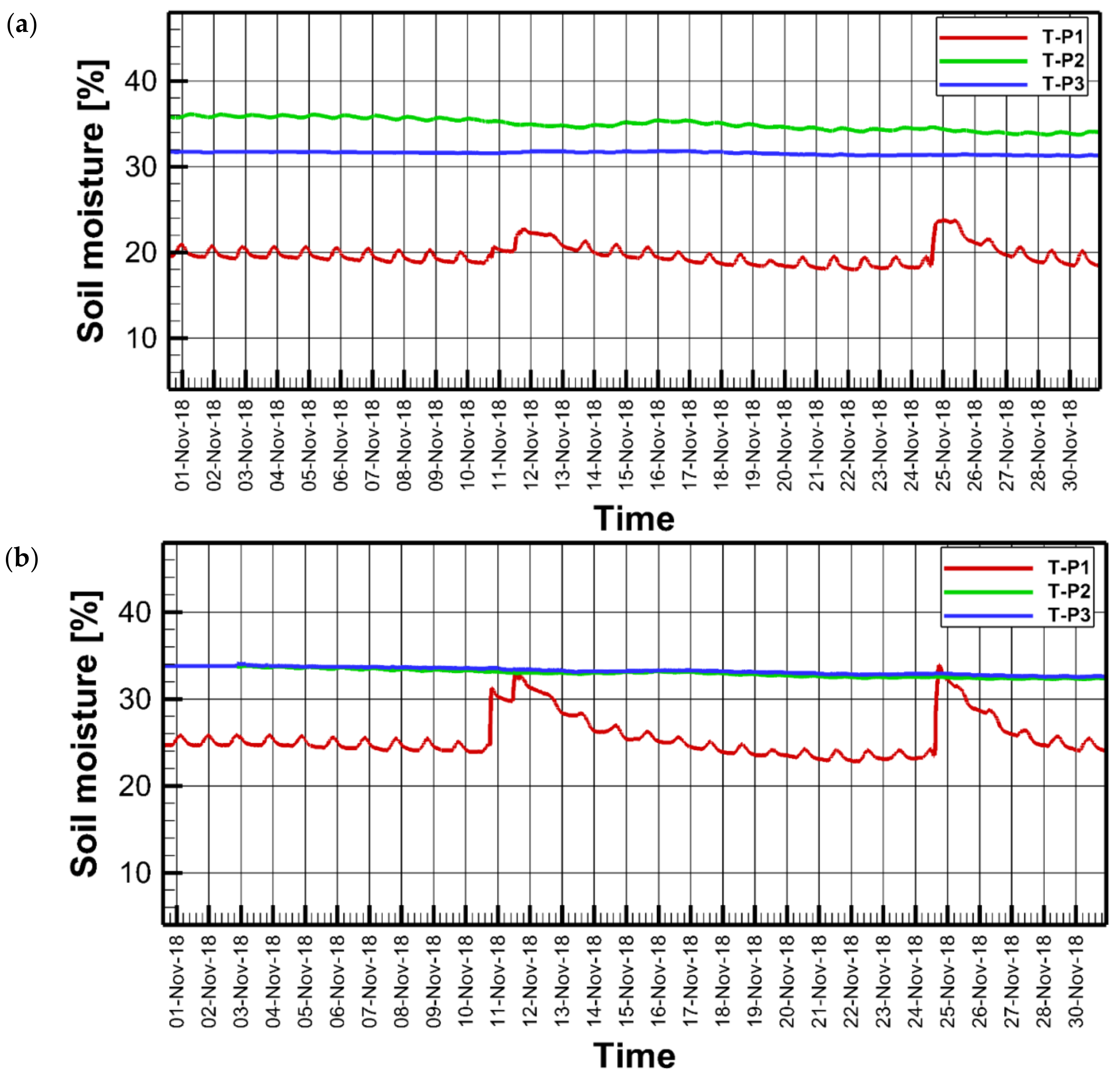
Two rainfall events occurred during November 2018: one on the 11th of November and another on the 25th (
Figure 6). The soil of lysimeter 1 showed a more pronounced response to rainfall than lysimeter 2 because of soil heterogeneity. Both rainfall events raised the soil moisture of the upper soil layer (i.e., probe 1), whereas the soil moisture at the deeper levels decreased slightly from their average levels during October. In both lysimeters, soil moisture of the topsoil declined to pre-rainfall levels after 3–5 days.
Table 2 presents the soil water balance for November. The net change in soil moisture at the end of November was −2.51 mm, based on balance weight data. The total evaporation was 19.91 mm, mostly sourced from meteoric water. Despite the deficit in soil moisture at the end of the month, some leakage occurred after rainfall.
3.3.2. December 2018 to March 2019
No rainfall occurred between December 2018 and March 2019. All evaporation during this period was therefore related to losses in soil moisture. The total monthly evaporation rates for December, January, February, and March were 2.15 mm, 2.34 mm, 2.49 mm, and 3.90 mm, respectively. No flow into the lysimeter occurred during these months. Evaporation in March was high, compared to January and February. This was because of the rapid increase in temperature during March (
Figure 4).
3.3.3. April 2019
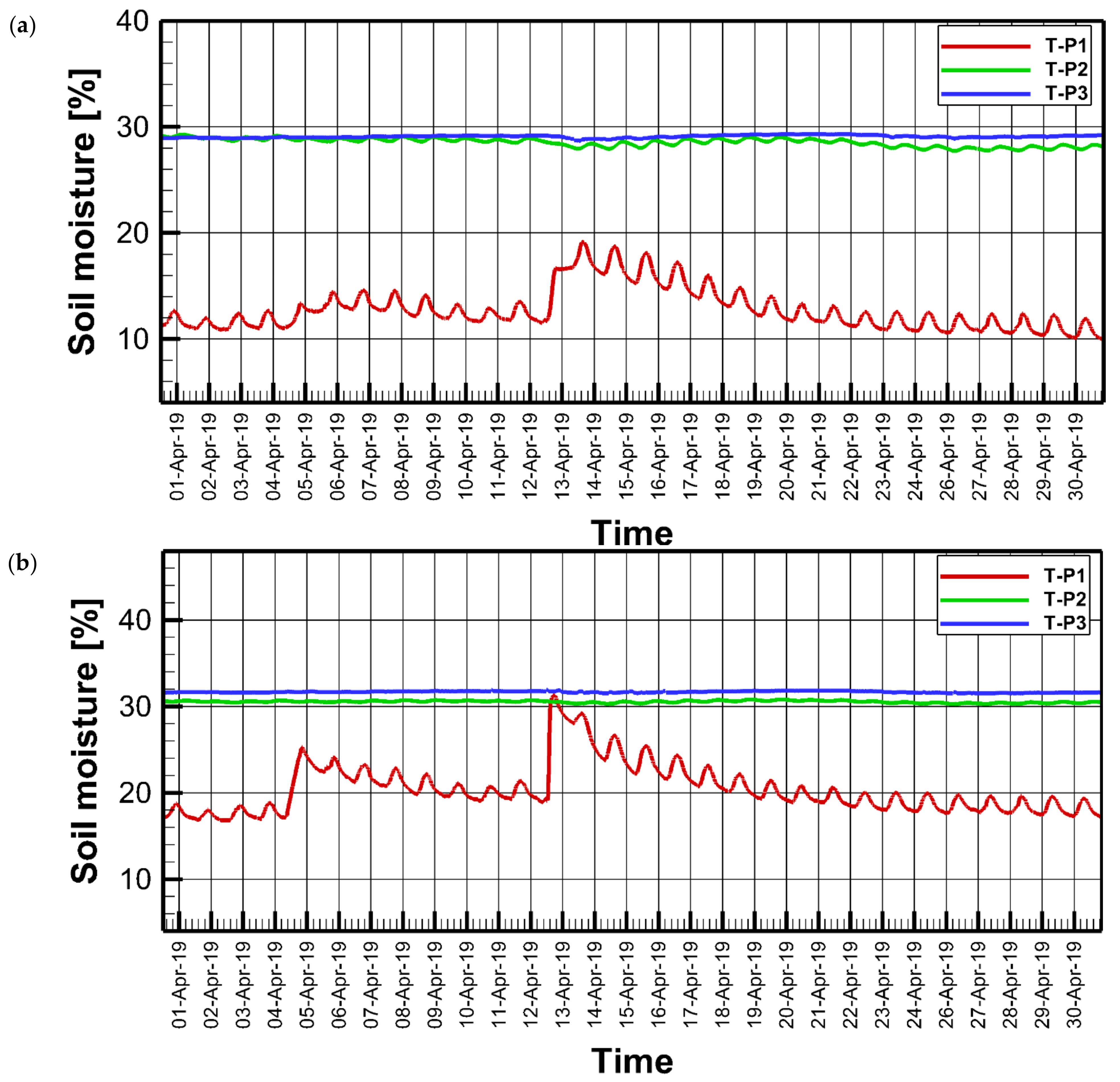
Figure 7 shows the soil moisture fluctuations during April 2019, which was the last month that witnessed rainfall in the hydrological year of 2018/2019. The total monthly precipitation was 11.90 mm, with rainfall occurring on the 5th and 13th of April. Soil moisture levels were generally lower than those observed during November and showed an overall decline, except from isolated spikes which occurred directly after rainfall events. Rainfall in April resulted in no leakage, as shown in
Table 3. All rainfall water and some of the soil moisture content was lost during this period due to evaporation. Overall, there was less evaporation in April compared to November because of the relative paucity of available water.
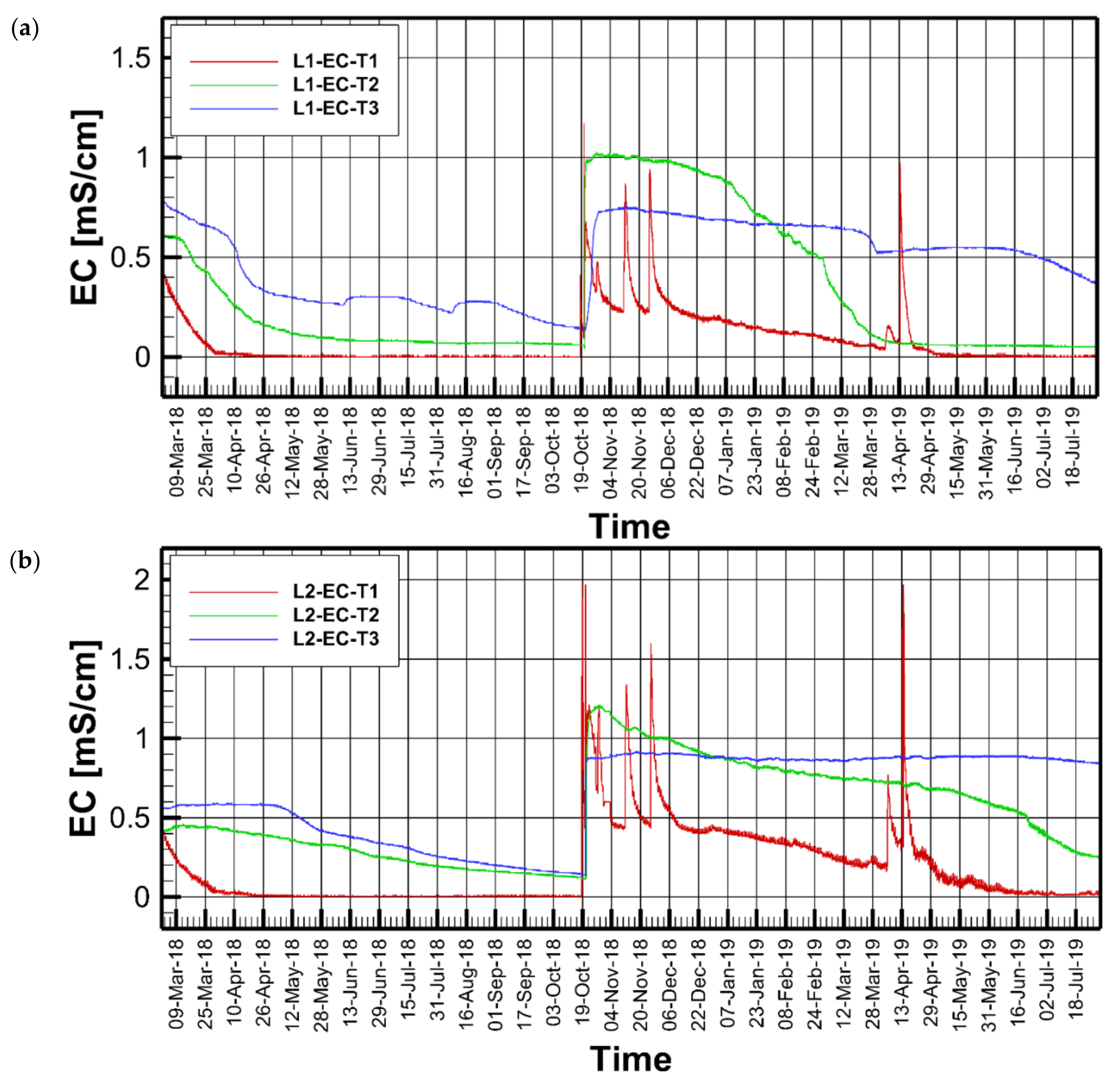
3.4. Electrical Conductivity (EC)
The electrical conductivity (EC) measures how soil can transmit an electric current, reflecting the salinity of the soil’s pore fluid. It is important to measure the EC in order to assess the health of soil for farming, as greater values indicate high salinity and thus poorer substrate conditions [
27]. If the EC is high, plants will not be able to take water via osmosis and will subsequently die. Many factors, such as temperature, soil moisture, and irrigation, affect EC measurements [
28,
29,
30]. In addition, soil pH, which is a measure of ionic content, affects EC. Highly acidic or basic soil translates to high EC values.
Figure 8 shows the bulk EC in the soil at T1 (5 cm), T2 (35 cm), and T3 (55 cm) for both lysimeter 1 and lysimeter 2 at 10-min increments from March 2018 to July 2019, showing a high degree of correlation with soil moisture (
Figure 5). The correlation factor between soil moisture and EC varied between 0.88 to 0.93, dependent upon the depth. Costa et al. [
29] found that the ideal time to measure EC was during periods of high soil moisture content.
After disregarding sensor noise at the very start of rainfall events, the EC varied between 0 and 1 mS/cm. EC values below 4 mS/cm were considered good for the plants. In both lysimeters, the measured EC in the shallow probe showed flat lines (i.e., EC = 0) when the soil was very dry. Values spiked at the beginning of rainfall, and then gradually declined as the soil moisture decreased. The middle and deep probes showed less fluctuation compared to the shallow ones. EC values at high moisture content were close to 1 mS/cm, reflecting true values.
3.5. Water Balance Analysis of the Wet Season
The wet season in Qatar extends from September to April (inclusive), but it is highly variable from one year to another because of high variability in rainfall. The dry season occurs from May to August. This section discusses soil moisture behavior during and after rainfall events and analyzes the leakage/evaporation during this period. These rainfall events occurred on the 18th, 20th, and 27th of October 2018; the 11th and 25th of November 2018; and the 5th and 13th of April 2019.
3.5.1. September 2018
No rainfall occurred during September 2018. The water balance calculations revealed a loss in soil moisture due to evaporation, given the high temperature at the end of the dry season. However, the evaporation rate during this month was reduced by a lack of moisture in the soil and an increase in air humidity at this time of the year. Using balance weight records, the total evaporation in September 2018 was 3.24 mm. The flow into the lysimeter from the water tank was 0.71 mm.
3.5.2. October 2018
October witnessed three rainfall events on the 18th, 20th, and 27th. Rainfall on 18 October 2018 was the first in the hydrological year 2018/2019, with a total precipitation of 11 mm.
Figure 9 shows the soil moisture behavior in October 2018. Before the rain event, day-and-night variation in soil moisture is consistent. During the night, soil receives moisture from the air as the overlying air becomes very dry during the day [
31]. This is reflected as an increase in soil moisture, as shown in
Figure 9. The soil moisture in the top-level (top 5 cm of soil) was less than 10% before the rain and increased sharply afterward. Lysimeters exhibited a different reaction to rainfall due to variations in soil hydraulic properties, e.g., lysimeter 2 showed a higher increase in soil moisture after the first rainfall event. In both cases, the deeper probes showed no change in the soil moisture after the initial episode of rainfall.
Soil moisture increased to field capacity (35%) at the beginning of the rainfall before declining. Rainfall of 11 mm at the beginning of the season affected only the top layer of soil without impacting the deeper reaches. No leakage/recharge occurred during this rainfall event. Eccleston et al., (1981) [
13] reported that a rainfall event of 10 mm or more may result in leakage/recharge. This was not the case in this instance, due to the undersaturated nature of the topsoil (top 5 cm).
On 20 October 2018, a significant storm hit Qatar, which brought heavy rainfall.
Figure 9 shows that the soil moisture increased to the highest level in all probes shortly after the storm. While the top probe showed a gradual decline in the soil moisture two days after the storm, it remained unchanged at the lower probes. Another rainfall event occurred on 27 October, which had various impacts on the topsoil moisture content of both lysimeters. Leakage analysis revealed that it started slowly in the unsaturated soil and continued for some time after rainfall ended (a delayed effect). The rainfall event on the 20th of October resulted in substantial recharge into the ground. Using Equations (1)–(4), leakage during October was found to be 6.71 mm. Similarly, based on Equation (4), the average monthly evaporation was calculated to be 29.39 mm or 0.68 mm per day. The increase in soil moisture content was calculated at the end of the month using the associated increase in the lysimeter soil column weight. It was found that the soil moisture increased by 35.21 mm.
Table 3 summarizes the water balance components for October 2018.
Table 3.
Monthly water balance for October 2018.
Table 3.
Monthly water balance for October 2018.
| Component | Value (mm) |
|---|
| Rainfall | 73.31 |
| Leakage | 6.71 |
| Evaporation | 29.39 |
| Change in soil moisture | 35.21 |
| Flow into lysimeter | 0 |
3.6. Water Balance Analysis of the Dry Season
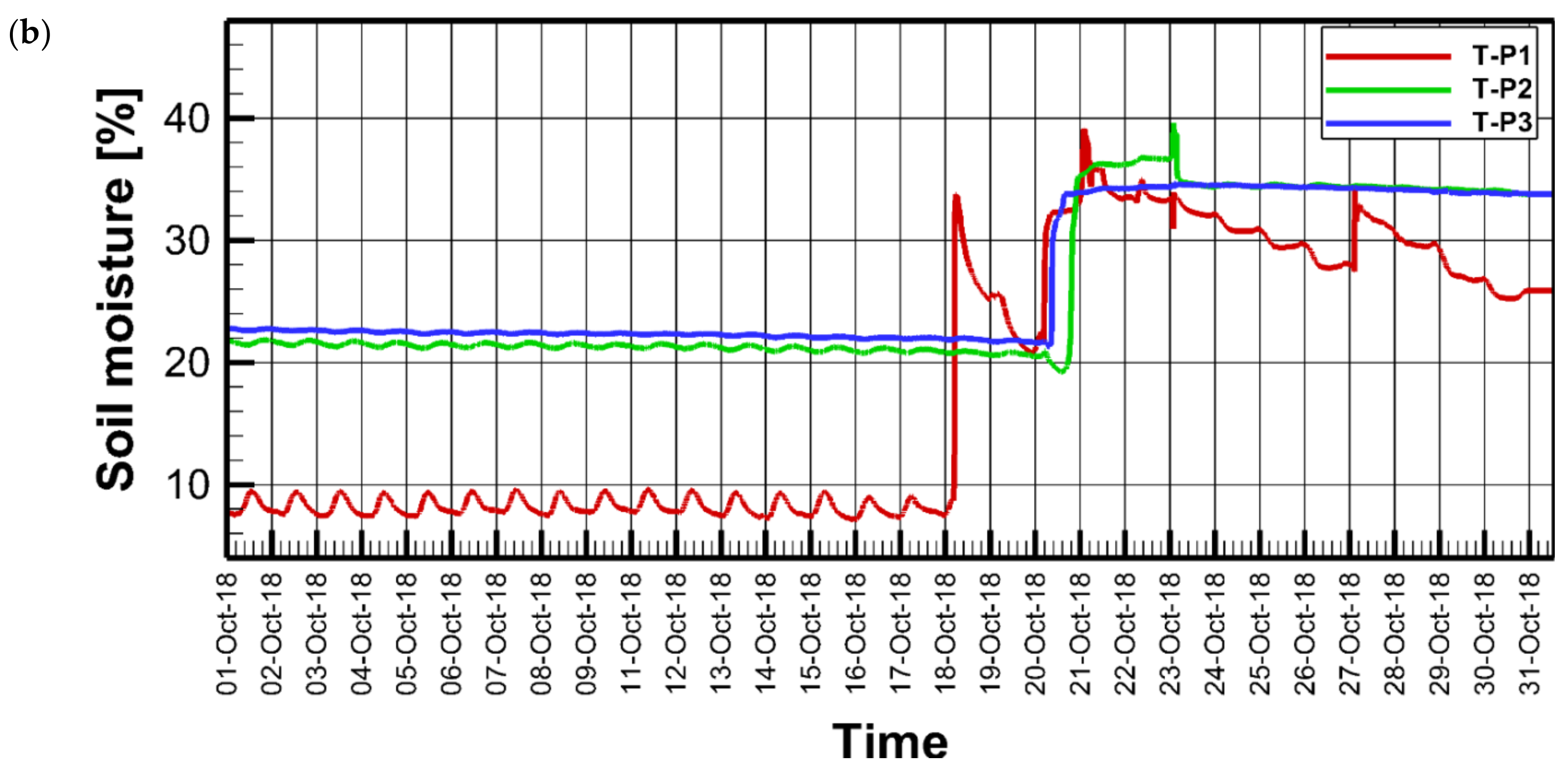
Figure 10 shows the soil moisture from the 1st of May to the 31st of July 2019. No rainfall occurred in that period, and soil water loss via evaporation represented the dominant component. It is remarkable that the soil moisture in the upper layer exhibited a sharp decline from the beginning of May to the end of June, and then declined less dramatically during July and August. This was because of the high air humidity during this period, which buffered evaporation rates. Evaporation in May was 5.98 mm, based on balance weight calculations, associated with a 2.7% reduction in the soil moisture content within the soil’s upper layer. Similarly, evaporation in June was 5.52mm. For July and August, evaporation rates were 5.12 mm, and 4.31 mm, respectively. It is notable that soil behavior in lysimeters 1 and 2 was markedly different. While lysimeter 1 had a relatively constant soil moister content for probe 2 and 3 (i.e., set at deeper levels), lysimeter 2 showed a decline in soil moisture at probe 2. We attributed this to the heterogeneity soil in their contained in the lysimeters. During these dry months, upward flow into the lysimeter occurred, namely 0.81 mm, 0.76 mm, 0.82 mm, and 0.73 mm for May, June, July, and August, respectively.
Table 4 summarizes the results of this study for the hydrological year 2018/2019. The table shows the monthly and the annual water budget.
3.7. Soil Matric Potential
The soil matric potential (SMP) is indicative of the cohesive force between soil particles and water molecules in the pore space of the unsaturated zone. Hence, it represents the force of attraction or tension between water molecules and soil. It provides an indication of the ease at which plants can uptake water from the soil, and is arguably the most important criteria for irrigation design [
32,
33,
34]. The higher the SMP, the more difficult it will be for plants to receive water from the soil. The SMP differs from soil moisture in the sense that the latter shows how much water is available in the soil, whereas the SMP represents the availability of water for plant growth. The SMP was measured at three locations in each lysimeter, namely at 50 mm, 350 mm, and 550 mm depths from the ground surface level. Because the top layer of soil was the most critical for plant germination and growth, we present data from the first probe.
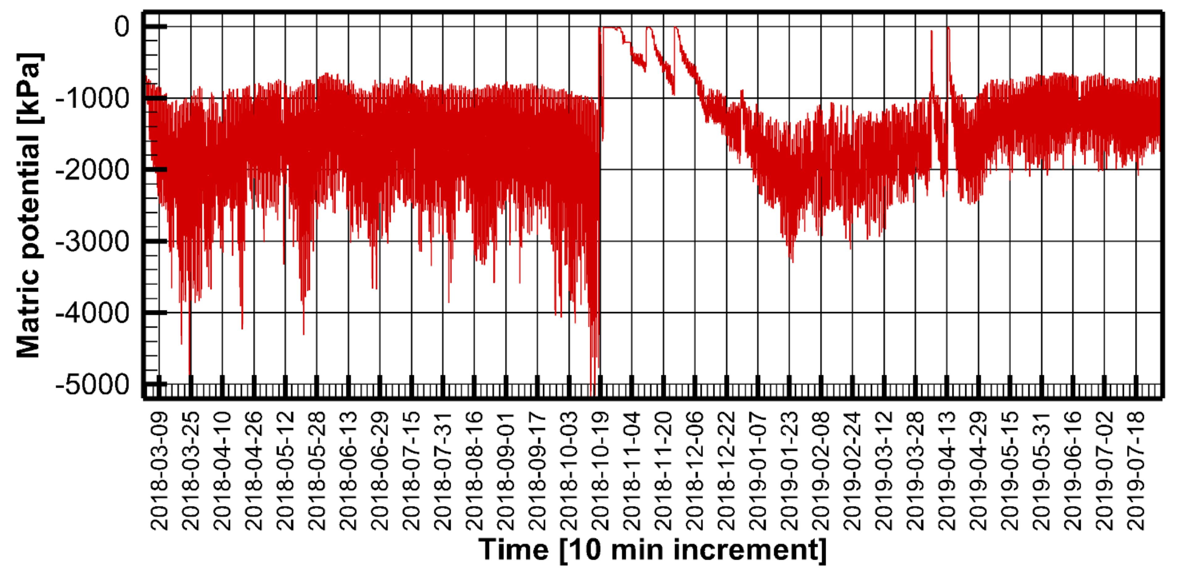
Figure 11 shows the SMP for the upper soil layer for the period between March 2018 and July 2019. The SMP varied between zero when the soil was fully saturated to around −5000 kPa when it was very dry. In such instances, negative values indicate suction. The SMP rose to 0 rapidly after rainfall and slowly dropped thereafter. After the first rain in the season (18th of October), the SMP rose to near-zero conditions when rainfall occurred, falling to −100 kPa over the course of a few hours. On the 20th of October, after the major storm described in
Section 3.4, the soil matric potential remained close to zero for over 20 days. Similar behavior occurred in November after rainfall. The SMP after rainfall during April was around −280 kPa, which was sufficient for plants to uptake water. For this soil, field capacity (FC) occurred when the SMP was ~−33 kPa. For loamy soils (i.e., the soil types examined by this study), the field capacity was about 35% of volumetric soil moisture. The SMP of −1500 kPa marked the permanent wilting point (WP); if no water was available, all plants would die. This occurred when the volumetric soil moisture ranged between 10% and 15% in the loamy soils. Obtaining the SMP was critical for irrigation management and water conservation, especially in arid zones where the water balance was highly tenuous in the context of plant germination and growth.
3.8. Model Results
Calibration results showed that
α = 0.029 and
n = 1.4. The model was run for summer and winter months to compare evaporation and drainage results with those obtained by the lysimeters. For summer simulation, moisture content data from tensiometers were used as input in Hydrus, and other parameters remained, as shown in
Table 5. For winter months, rainfall was inputted as a boundary condition when applicable. In all simulations, potential evapotranspiration data from [
14] were used.
Table 5 shows the Hydrus model results of monthly evaporation measurements versus lysimeter measurements. While rainy months (October 2018 and April 2019) showed a good match between measured and modelled evaporation, summer months of July and August 2018 showed that the model results were less than measured. The reasons for this could be related to uncertainty in model parameters that seem to affect summer months more than winter months. This includes the van Genuchten model parameters (
α and
n) and the potential evaporation. In all cases, the discrepancy of the model result and the lysimeter measurement was small.
4. Conclusions
The results presented above provide insights into the true surface evaporation, compared to previous studies that rely on pan evaporation or empirical formulae. Values of monthly evaporation varied between 2.15 mm in December to over 29 mm in October. While summer months (May–September) in Qatar witnessed high temperatures, the evaporation rate ranged from 4 to 6 mm per month, which was far less than potential values, due to low soil moisture content during this period. The highest observed evaporation rates were in October, November, and April, as rainfall occurred during these months. It is notable that most of the rainfall in these months was exchanged back into the atmosphere by evaporation, with a minor fraction being able to leak down to the lower layers. The flow from the water tank into the lysimeter, which mimics capillary rise in unconfined soil substrates, occurred during dry months only, providing a temporal framework for the preponderance of capillary flow.
The total rainfall in the study area during 2018/2019 was 102.73 mm, which is higher than the country’s long-term average of 80 mm. The actual total annual evaporation was 97.63 mm, which is 95% of the total rainfall. The total input via the leakage minus the flow into the lysimeter was 5.1 mm (i.e., the remaining 5% of the rainfall).
Despite the fact that the studied soil profiles were taken from the same area with a separation of ~100 m, the behavior in each lysimeter was markedly different. Lysimeter 2 showed a greater response to rainfall events and stronger spikes than the first lysimeter. This reflects the high intrinsic heterogeneity of the soil within lysimeter 2’s location.
Between April and September, the upper soil was completely dry (excluding potential anomalous rainfall events). The lowest soil moisture (for the loamy soil studied herein) was around 6% by the end of summer. The moisture contents of the lower soil layers fluctuated between ~10% during summer to ~20% during winter. This percentage increased to field capacity immediately after rainfall events. In the hydrological year 2018/2019, the first rain in the season was insufficient to infiltrate into the lower soil, but was still able to partially saturate the upper soil. When high magnitude rainfall events occurred over short periods (i.e., >10 mm over the course of a few hours), leakage was likely to occur (e.g., during late October and November 2018). The rainfall event during April provided 11.9 mm of water but generated no leakage into deeper soil layers. This was due to the presence of dry topsoil at this time, meaning that the amount of rainfall was sufficient to wet the upper soil layer only. During this time, all received rainfall was lost to evaporation, in addition to a slight decrease in soil moisture.
The SMP was generally very low (<−1000 kPa), which does not support rainfed agriculture. Only after October and November could the SMP be considered high enough to support plant growth several days after rainfall. This meant that irrigation was necessary to support agriculture, even during the wet season.
Actual evaporation tended to be much lower than potential evaporation in arid areas, due to low rainfall and scarcity of soil moisture. Despite the low rainfall, leakage to deep soil layers occurred if some conditions were met, including the residual wetness of the upper soil after the dry season and the quantity of rainfall received. If rainfall occurred when the upper soil was already wet by previous rainfall, then leakage can occurred. In this study, the 11.6 mm of water provided by the first rainfall of the hydrological season was useful to replenish moisture content of the soil, though no recharge occurred. During wet and cold periods (i.e., January and February), 10 mm of rainfall was expected to induce groundwater recharge. The rainstorm on the 20th October created significant flooding, resulting in ponded water in many areas, giving rise to significant recharge over the following hours. Leakage continued beyond the storm time due to what is known as the ‘delayed effect’. Elevated topsoil moisture attributable to these high magnitude rainfall events (i.e., >10 mm rainfall) tended to diminish over 2–3 days. The calculated leakage to deep soil layers was around 5% of the total rainfall, whereas evaporation accounted for the remaining 95%. These results are useful for water balance analysis, the study of soil moisture dynamics in arid zones, and irrigation management in such settings. The lysimeter data were validated through modelling, showing a good match between the Hydrus model and lysimeter evaporation data. Future research should focus on expanding the study of lysimeters to include more soil types and wider geographical distribution.


