
Response of Low Flows of Polish Rivers to Climate Change in 1987–1989

1
Department of Hydrology and Water Management, Faculty of Geographical and Geological Sciences, Adam Mickiewicz University, Bogumiła Krygowskiego str. 10, 61-680 Poznań, Poland
2
Association of Polish Climatologists, Krakowskie Przedmieście str. 30, 00-927 Warsaw, Poland
*
Author to whom correspondence should be addressed.
Water 2022, 14(18), 2780; https://doi.org/10.3390/w14182780
Submission received: 25 June 2022
/
Revised: 21 August 2022
/
Accepted: 5 September 2022
/
Published: 7 September 2022
(This article belongs to the Special Issue Climate Change Impact on Hydrological Cycle and Water Resources Management)
Abstract
:The paper discusses changes in the low-flow regime of rivers in Poland, resulting from climate change that occurred between 1987 and 1989. The low-flow variability of rivers was measured with the use of the number of days with low flows (NDLF) below a threshold value, which was adopted as the 0.1 (10%) percentile (Q10) from the set of daily flows recorded in the multi-annual period 1951–2020 at 140 water gauges on 83 rivers. The analysis of the course of climate change over Poland showed that it was caused by macro-circulation conditions, controlled by changes in the intensity of thermohaline circulation in the North Atlantic (NA THC). Climate change consisted of a sharp increase in sunshine duration and air temperature, and a decrease in relative humidity after 1988. Along with the lack of changes in precipitation totals, characterized by a strong yearly variability, and an increase in field evaporation, it led to noticeable changes in the water balance. As a result, in 1989–2020, there was a significant increase in NDFL detected in about 2/3 of the area of Poland. With the change in the NA THC phase and the macro-circulation conditions, there was also a change in the spatial distribution of areas drained by rivers with increased NDFL. In 1951–1988, these included the eastern parts of Poland, while after the climate change (1989–2020), its western and south-western parts.
1. Introduction
Between 1987 and 1989, the macro-circulation conditions in the Atlantic-European circulation sector changed, which led to climate change over Europe. In Poland, this change was most clearly marked by an abrupt increase in sunshine duration and air temperature, as well as a change in the cloud structure and a decrease in relative humidity. Moreover, the structure of the winter NAO index changed toward an increase in the frequency of positive index values, and the annual geopotential increased significantly over Poland. The annual precipitation totals remained unchanged, within the range of their current, significant inter-annual variability.
An increase in air temperature and sunshine duration, and a decrease in relative humidity are factors influencing an increase in field evaporation (e.g., [1,2,3]), which should be reflected in shaping the water balance change. In turn, the water balance change should be reflected in the change in river flow regime, which particularly clearly manifested in an increase in the frequency of occurrence of low flows.
Correlations analyses with indices quantifying large-scale climate variability have been performed by many authors. For the European region, the most relevant modes of climate variability appear to be the North Atlantic Oscillation (NAO) and the Atlantic Multidecadal Oscillation (AMO) [4].
Shorthouse and Arnell [5] confirmed that during winter positive NAO phases, winter stream flows were generally higher in Northern Europe, and lower in Southern Europe, while the authors of [6] proved that hydrological regimes most sensitive to NAO variations were located at the Northern and Southern extremities of Europe, i.e., in the Scandinavian and in the Iberian peninsulas. A few other studies focused on specific European regions, such as the British Islands [7,8] and Scandinavia [9]. On a country scale, the authors of [10] determined that a negative phase of winter NAO was generally followed by a negative anomaly of fall stream flows in England and Wales, while the authors of [11] concluded that positive phases of winter NAO were usually associated with pronounced summer droughts in Romania. Giuntoli et al. [4] analyzed low flows in France in relation to large scale climate indices and found that seasonal climate indices had stronger links with low-flow indices than their annual counterparts.
Until now, various studies on the hydrology of droughts and low flows on rivers in Poland paid little attention to the existing climate change, treating the hydrological conditions prevailing after 1951 as stationary, and the interest in the frequency or percentage of low flows during the year resulted to a greater extent from treating them rather as a measure of the occurrence of hydrological drought [12,13,14,15,16,17,18,19]. Szwed et al. [20] studied the effects of climate change on agriculture, water resources, and human health sectors in Poland, and the authors of [21] applied three drought indices: the Standardized Precipitation Index (SPI), Standardized Precipitation Evapotranspiration Index (SPEI), and Standardized Runoff Index (SRI), and the hydro-climatic data to hydro-meteorological drought projections into the 21st century for selected Polish catchments.
Therefore, the problem is whether the occurring climate changes have an impact on the water balance in Poland, and to what extent these changes in the water balance have an impact on the flow regime in Polish rivers.
The aim of this paper is to present the results of research on the change in the frequency of occurrence of low flows in Poland in the multi-annual period 1951–2020 divided into two sub-periods, treated as different phases of the climate change: In 1951–1988 preceding climate change, and in 1989–2020 following that change. The research focuses on two aspects of this variability, i.e., the variability that occurred as a function of time, and the changes in the number of days with low flows that occurred in space. The hydrological part of the study is preceded by a short discussion on the most important manifestations of changes in selected elements of climate, important in terms of shaping the water balance, and changes in the water balance that occurred in Poland as a result of climate change that took place in 1987–1989.
2. Materials
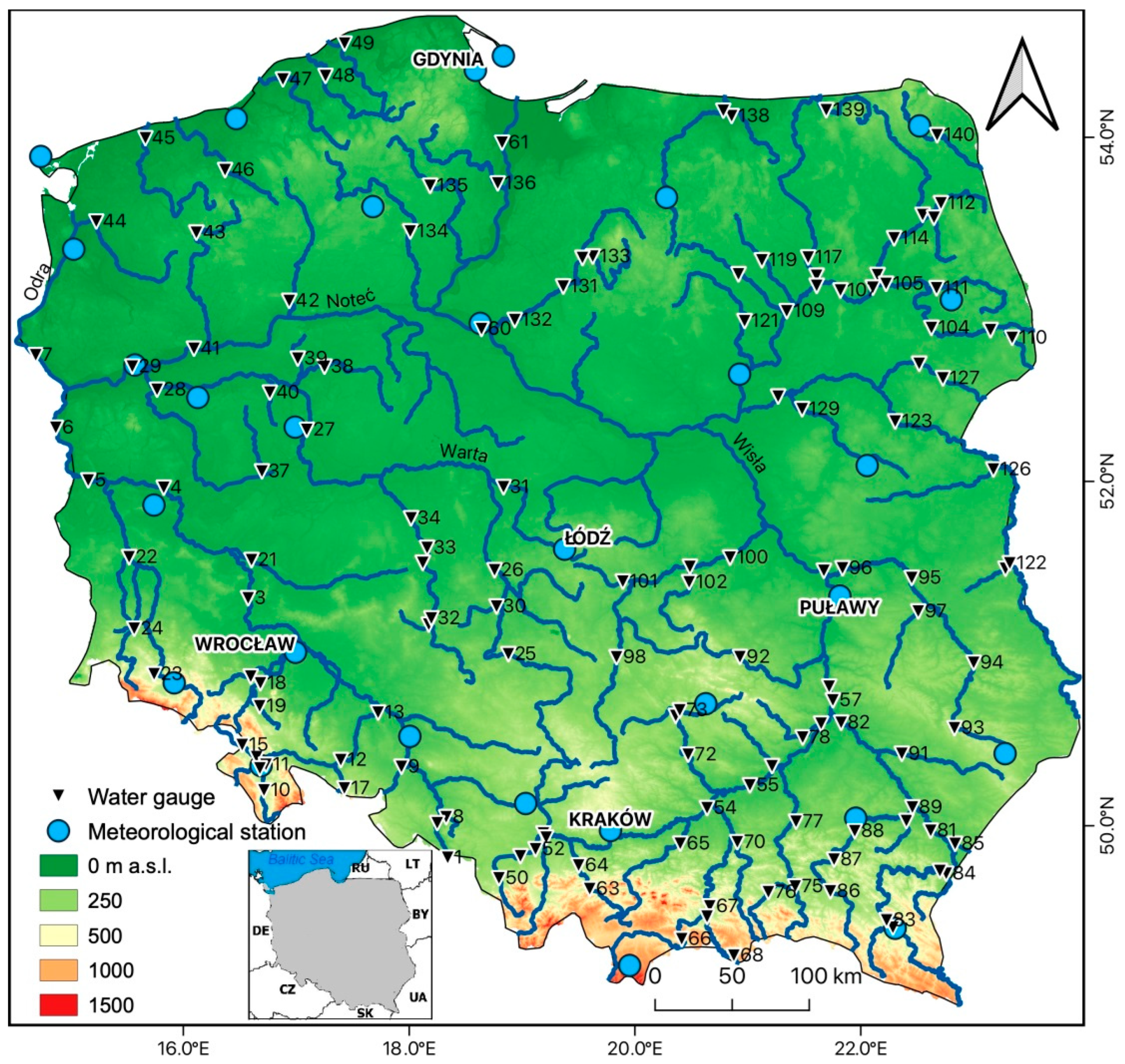
The hydro-meteorological data were obtained from the database of the Institute of Meteorology and Water Management–National Research Institute (IMGW-PIB) in Warsaw [22]. The analysis is based on the series of annual air temperature (T), annual precipitation totals (P), annual values of general cloudiness (N, 1/8), and annual values of relative humidity (f, %). In this study, the authors used the values of the above-mentioned climatic elements, which constituted the area averages of 28 stations that were relatively evenly distributed in Poland (Figure 1) and covered the multi-annual period 1951–2020. In order to indicate that these values were the area averages, they were respectively marked as TPL, PPL, NPL, and fPL in this paper.
The number of days with low flows (NDLF) per year on Polish rivers was calculated based on the publicly available data of daily flows recorded at 140 water gauges on 83 Polish rivers in the multi-annual period 1951–2020 [22]. The geographical position of the analyzed water gauges is presented in Figure 1 and basic hydrological data on the studied rivers are shown in Table A1.
The number of annual sunshine duration (marked as SDPL) was the average of five stations: Gdynia, Łódź, Kraków, Wrocław, and Puławy (Figure 1), and covered the period 1951–2018. Data from the Wrocław station were the combined sequences of the sunshine duration observations from the stations of the University of Wrocław (station Biskupin) and the University of Life Sciences in Wrocław (station Swojec). The combination of the two ranks and their homogenization was carried out by the authors of [23]. The data from Kraków station were the continuous, fully homogeneous observatory series from the IGiGP observatory of the Jagiellonian University [24,25]. The series from Łódź station combined the data published from 1951–2000 by the authors of [26] with the data from IMGW-PIB (2001–2018). The data from Puławy station were derived from the IUNG observatory in Puławy, while the data from Gdynia were obtained from the IMGW-PIB station. The limited series of annual sunshine duration used to calculate the area average was justified by the fact that the sunshine duration data provided by IMGW-PIB started from 1966.
The time sequences of the frequency of the macro-types of the mid-tropospheric circulation according to the Wangengejm-Girs classification, compiled by the Arctic and Antarctic Research Institute (AARI), St. Petersburg, RF, covering the period from January 1951 to March 2018 were obtained from Appendix No. 2 to the study implemented by the authors of [27]. The remaining parts of the sequences, until December 2020, were obtained directly from AARI.
Additionally, the work used the time series of the geopotential height of the isobaric surface of 500 hPa (h500) and the similar series of pressure at sea level (SLP) with a monthly resolution from selected grids. The annual values of h500 and SLP for individual grids were calculated as simple arithmetic means of monthly values in a given calendar year. Both types of data were obtained from NCEP/NCAR reanalysis [28] and were downloaded from NOAA/OAR/ESRL PSL, Boulder, Colorado, USA, from their website at https://psl.noaa.gov/data/gridded/data.ncep.reanalysis.pressure.html (accessed on 12 January 2021).
3. Methods
The values of field evaporation (Ev, mm of water column equivalent) in a given month from the area of Poland were calculated using the Ivanov formula (after [29]):
where t is the monthly average temperature (°C), f is the monthly relative humidity (%), in which arguments of function (1) are the area means of TPL and fPL. Annual field evaporation was calculated as the sum of monthly evaporation. The method of estimating field evaporation using the formula proposed by Ivanov is considered to give the most realistic results and performs satisfactorily in Poland (e.g., [3,30,31,32]). Using a series of annual Ev values, the approximate water balance in a given calendar year was estimated as the difference between annual precipitation (PPL) and annual evaporation (Ev), without taking into account retention.
Ev = 0.0018 × (25 + t)2 × (100 − f),
The threshold level method is one of the most widely used in hydrological analyses of low flows. In this method, low flow is defined as the period during which the flows are equal to or lower than the adopted threshold value [33]. However, the criteria for establishing that threshold values are not clearly defined in scientific literature, and are taken arbitrarily depend on the researcher. Among the statistical criteria, the value of the Qp percentile with the assumed exceedance probability is determined, calculated on the basis of the sum flow curve (integral curve) plotted at the individual water gauge for the studied period. The most common p-values are 90 and 95 [34].
In our research, we used the 10th percentile (Q10) from the sum flow curve with the lower values, which corresponds to the 90th percentile (Q90) from the sum flow curve with the higher values. The low-flow periods were characterized with the use of the number of days with low flows (NDLF) below a threshold value, which was adopted as the 0.1 (10%) percentile (Q10) from the set of daily flows in 1951–2020. The duration of low flows was calculated for the entire multi-annual period 1951–2020 and two sub-periods: Before (1951–1988) and after climate change (1988–2020). In the next stage of the analysis, the change trends in the number of days with flows below Q10 detected at the respective water gauges and their statistical significances were determined. The differences in the duration of low flows below Q10 between the period after climate change (1988–2020) and before it (1951–1988) were also calculated.
In order to get in more detail into the structure of NDLF variance and to explain the connections between NDLF at individual water gauges, the set of the NDLF time series was analyzed with the help of the Principal Component (PC) method. The use of the PC method is justified by the fact that the time series of the number of days with low flows at individual water gauges shows the differentiated strength of correlation, the vast majority of which are statistically significant and highly significant. Additionally, in this study, the long series of data are correlated with each other, and the PC method allows for the reduction in the number of analyzed variables, and for the detection of the variance structure and general regularities in the relationships between these variables.
The variance structure of NDLF was determined based on the analysis of the eigenvector relationships between five area climatic elements (precipitation—PPL, temperature—TPL, relative humidity—fPL, general cloudiness—NPL, sunshine duration—SDPL) and the annual area evaporation (EvPL) and two large-scale climate indicators, i.e., the winter (DJFM) Hurrell NAO index (PC-based) and the DG3L index, informing about the intensity of thermohaline circulation in the North Atlantic.
The mathematical and statistical processing of analysis results employed the statistical procedures included in the following software: Excel (Microsoft, Redmond, WA, USA) and Statistica 13 (TIBCO Software Inc., Palo Alto, CA, USA). The implementation of the graphic form employed QGIS (3.6.2. Noosa) and Surfer 10 (Microsoft, Redmond, WA, USA) software. The kriging procedure was applied for the construction of isolinear maps.
4. Changes in Climatic Conditions in 1951–2020 and Their Scope
4.1. Changes in Macro-Circulation Conditions
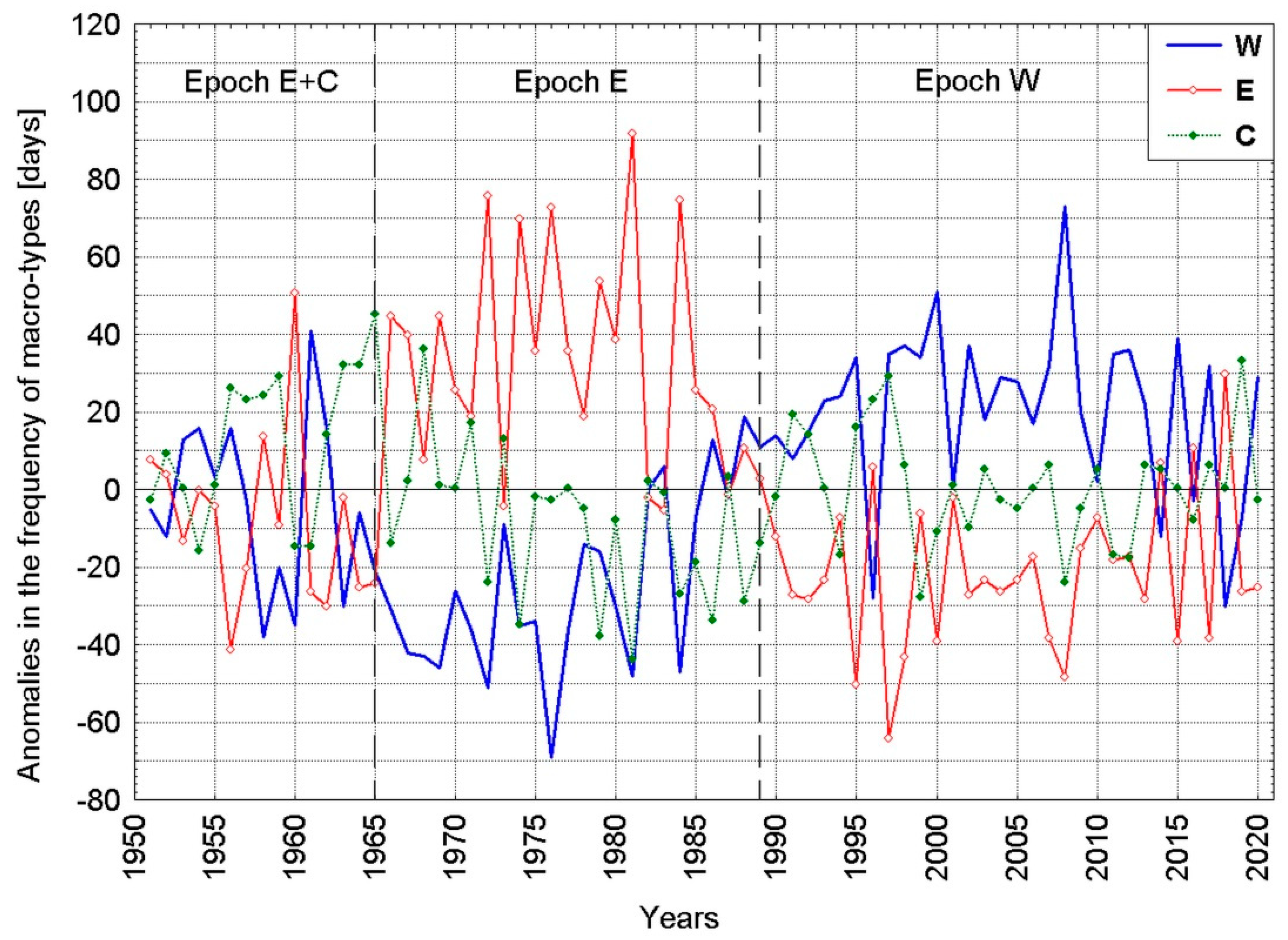
The macro-circulation conditions in the Atlantic-Eurasian circulation sector are determined by the frequency of the mid-tropospheric circulation macro-types (500 hPa) W, E, and C, according to the Wangengejm-Girs classification [35,36]. The annual frequency of these macro-types for the periods of several or several dozen years maintains certain features of the stability of the proportions between them, with the dominance of a specific macro-type or the dominance of one and sub-dominance of another macro-type, creating the so-called “circulation epochs” [37].
In the 70 years of the multi-annual period 1951–2020 analyzed in this study, the macro-circulation conditions in the Atlantic-Eurasian circulation sector changed twice (Figure 2). In 1965–1966, there was a transition from the circulation epoch E + C into epoch E, and in 1989–1990, from epoch E into epoch W [38]. Similar boundaries between these circulation epochs, showing a 1–2-year shift in time in relation to the separations proposed by the authors of [38], were determined by the authors of [39,40], who used different methods of their delimitation. (The transition from one circulation epoch to the next one is not immediate and takes several (3–4) years, in which the frequency of the dominant macro-type decreases to the long-term mean values and then drops below this value, and is replaced by another macro-type, gradually increasing above its long-term average. Depending on the adopted delimitation method and the length of the analyzed datasets, researchers may obtain different moments of “transition” from one to the next epoch).
After 1988, the frequency of the meridional macro-type E fell sharply below its long-term mean value, while the frequency of the zonal macro-type W increased noticeably, significantly exceeding the long-term mean values, and the frequency of macro-type C remained slightly below its long-term average; this state lasted until 2020 (Figure 2). The transition from the circulation epoch E into epoch W in 1987–1989 resulted in an abrupt change in the structure of the macro-types frequency.
Since the change in the structure of macro-types between individual circulation epochs was abrupt, it also forced simultaneous abrupt changes in the value of climatic elements, as the variability of the mid-tropospheric circulation controls the variability of the lower atmospheric circulation (SLP), and thus the weather structure. These changes in the mean values of climatic elements and their variability ranges, in the light of the definition of the climate by the authors of [41], can be interpreted as climate change.
4.2. Changes in the Course of Climatic Elements in Poland in 1951–2000
The analysis of annual changes in the area values of climatic elements and their distributions in respective circulation epochs shows that their changes between the circulation epoch E + C and epoch E (1965–1966), although noticeable, in most cases were not statistically significant. On the other hand, the changes of most climatic elements during the transition from the circulation epoch E into epoch W, which took place between 1987 and 1989, were highly significant. This prompts the conclusion that climate change occurred in these years.
In this paper, the characteristics of changes in the course of climatic elements will be limited to their presentation on the scale of the annual area averages and to these elements that have the strongest impact on the water balance. The value of the annual average of a given element is a synthesis of monthly and seasonal changes taking place in a given year.
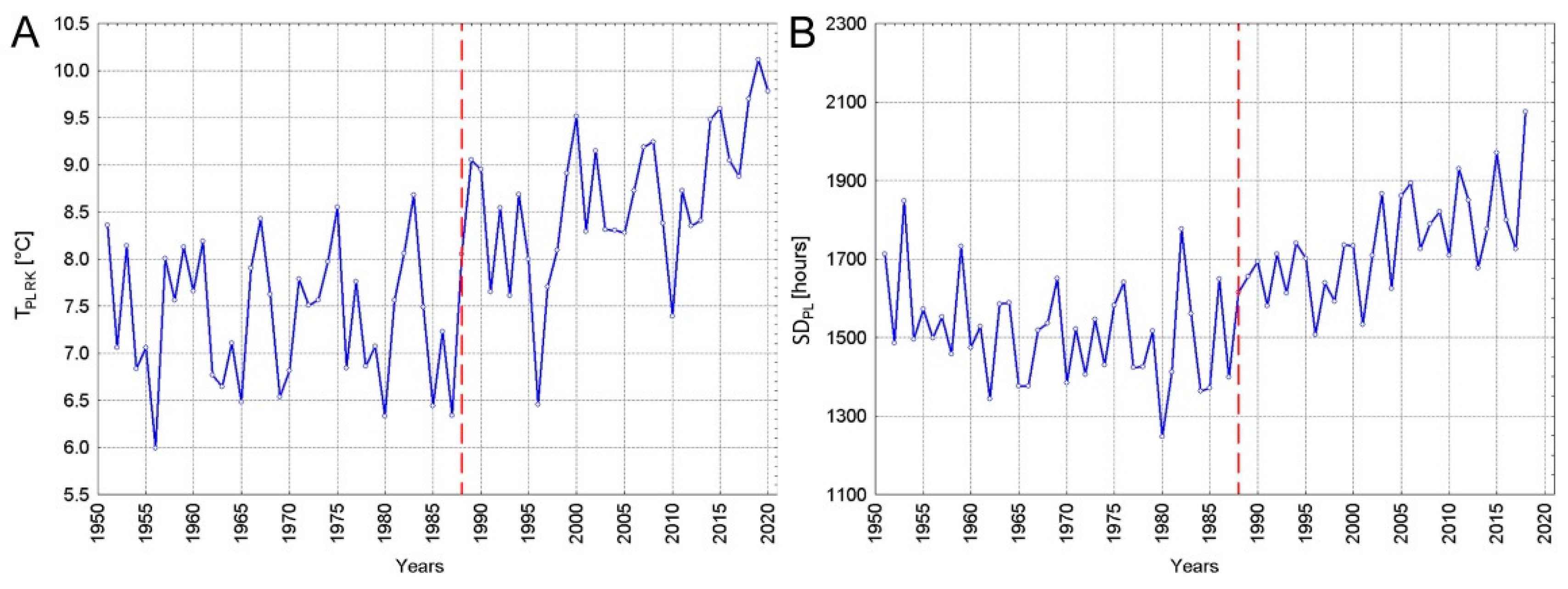
Air temperature in the multi-annual period 1951–1988, despite the change in circulation epochs from E + C into E and significant inter-annual variability, did not show statistically significant long-term changes. Its trend in 1951–1988 was nearly zero (−0.0025 (±0.0105) °C × year−1, p = 0.813). Between 1987 and 1989, there was a “leap” in the temperature increase by slightly more than 1°, and then a positive, statistically significant trend appeared in its course (+0.0420 (±0.0123) °C × year−1, p = 0.002). The course of temperature noticeably changed after 1988 (see Figure 3A), which is particularly visible in the course of the lower envelope of its variability band. The annual temperature course indicates that until 1988, despite very high inter-annual variability, no increase in temperature over Poland was observed (analysis of the temperature changes in Poland covering the period 1931–2020 shows that in 1931–1988 (58 years), despite very high inter-annual variability, the trend was zero), and a warming exceeding 2° by 2020, did not begin until after 1988.
Changes in sunshine duration were similar to the temperature changes. The time series is also non-stationary, and the period of its discontinuity can be found between 1987 and 1989 (Figure 3B), when there was a clear “leap” in the course of sunshine duration and then a positive trend appeared. It occurred along with the transition from the circulation epoch E into epoch W, while the transition from the circulation epoch E + C into epoch E did not cause statistically significant changes in the annual sunshine duration. In 1951–1988, the annual sunshine duration trend was negative (−2.76 (±1.88) hours × year−1) and statistically insignificant (p = 0.150), while in 1988–2018, the trend became positive (+9.11 (±2.02) hours × year−1) and highly significant (p << 0.001). Even a stronger relative increase in sunshine duration in 1987–1989 can be concluded when considering the changes in sunshine duration in the warm half-year (April–September), i.e., during the “long-day months”. In the course of the warm half-year sunshine duration, both the value of the “leap” and the positive trend after 1988 are stronger than the course of annual values. This indicates that the fundamental changes in sunshine duration between the two sub-periods took place in the warm half-year [42].
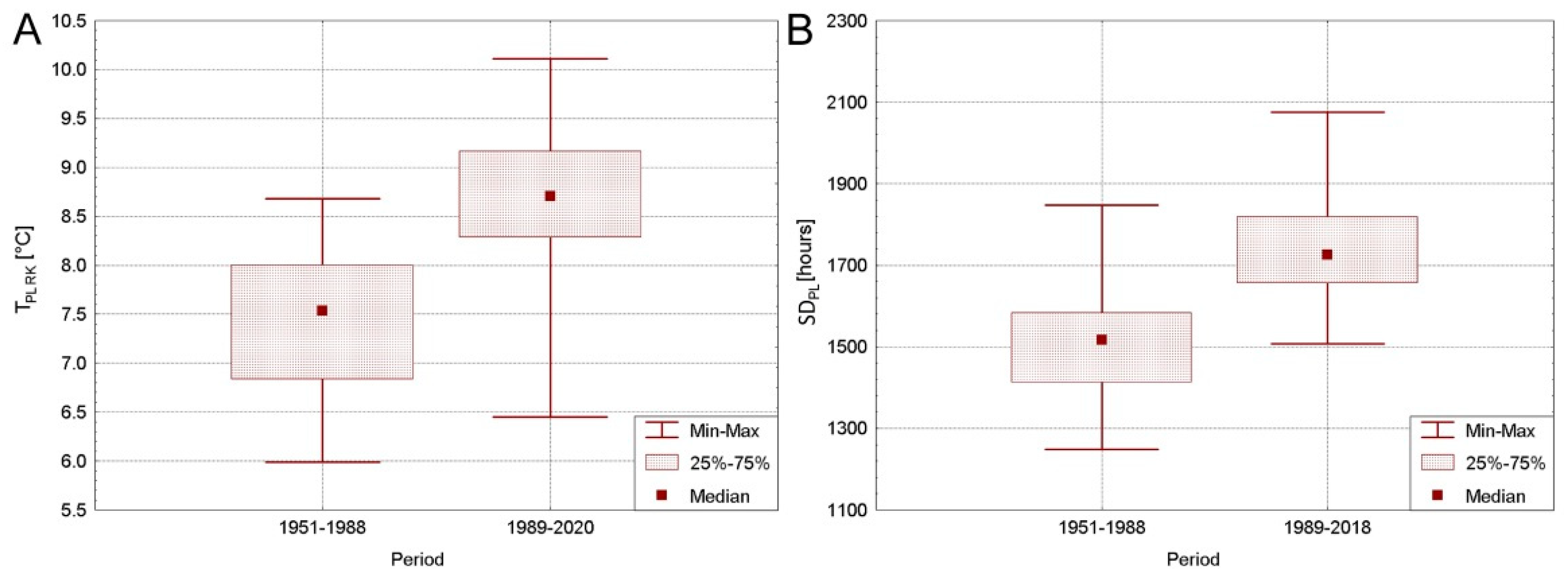
The changes in the range of variability in temperature and sunshine duration between the two sub-periods are significantly strong, in which the values of these two climatic elements in each analyzed sub-period resulted in statistically separate populations (Figure 4).
Moreover, the annual area relative humidity in Poland, that very strongly correlated with TPL and SDPL, shows clear differentiation in the analyzed two sub-periods. While the mean values of fPL in these sub-periods differ slightly (80.85 and 79.37%), the distributions of the fPL values are clearly different. The analysis of differences between the means of the sub-periods 1951–1988 and 1989–2020 shows that the differences between these means are highly significant (p = 0.0001 in the one-tailed test and 0.0003 in the two-tailed test).
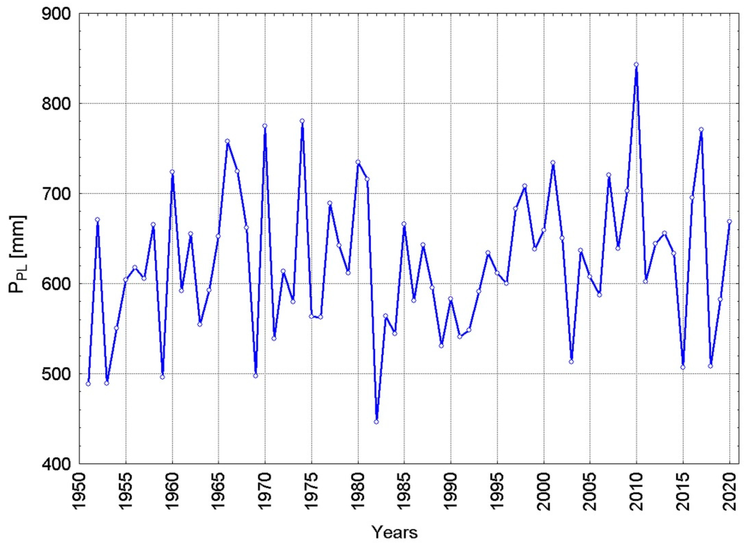
The course of the annual area precipitation totals in the whole analyzed period shows a weak and statistically insignificant positive trend (+0.63 (±0.48) mm × year−1, p = 0.191; Figure 5), and does not show discontinuities in 1987–1989, despite a temporary decrease in the annual precipitation totals in 1986–1993. The calculated differences between the mean annual precipitation in the two sub-periods (617.0 and 632.2 mm, respectively) are insignificant. On the other hand, the distribution of the annual precipitation totals changed in the second sub-period compared to the first sub-period: The annual precipitation maxima increased to 843 mm in 1989–2020 compared to 780.3 mm in 1951–1988, and the annual minima to 506.8 mm compared to 446.1 mm, respectively. This change in the range of variability of the maxima can be explained by the increased frequency of convective precipitation in the sub-period 1989–2020, with significant sums of precipitation recorded during individual rainfall episodes.
4.3. Changes in the Water Balance
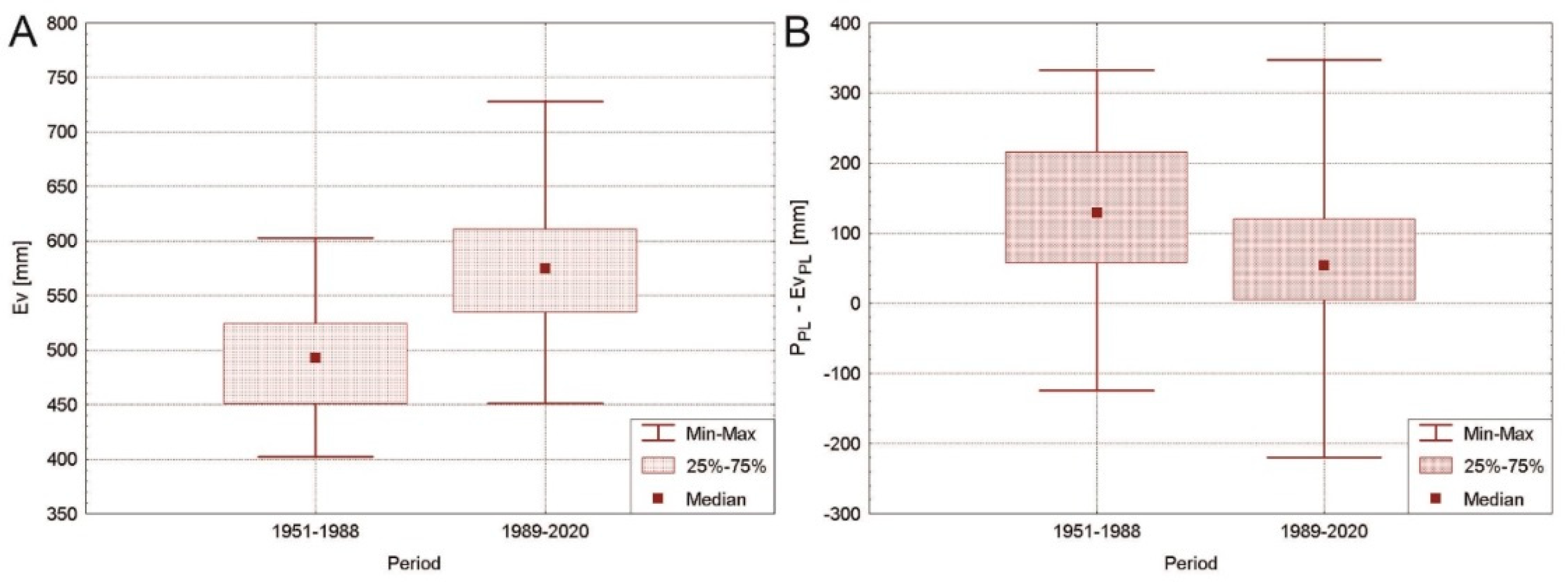
The annual area evaporation (EvPL) calculated with the use of method proposed by Ivanov in the two sub-periods show significant differences: In 1951–1988, it was an average of 493.4 mm, while in 1989–2020, this value increased to 579.1 mm. The variability ranges of the inter-annual evaporation also changed. In 1951–1988, the minimum EvPL reached 401.8, and the maximum 602.8 mm, while in 1989–2020, both extreme values increased: The minimum EvPL was 451.1 mm, and the maximum 728.0 mm. Therefore, in 1989–2020, the amount of water losses on evaporation increased very strongly in Poland compared to 1951–1988, and the variability of the evaporation values calculated for each of these sub-periods also created two separate populations (Figure 6A).
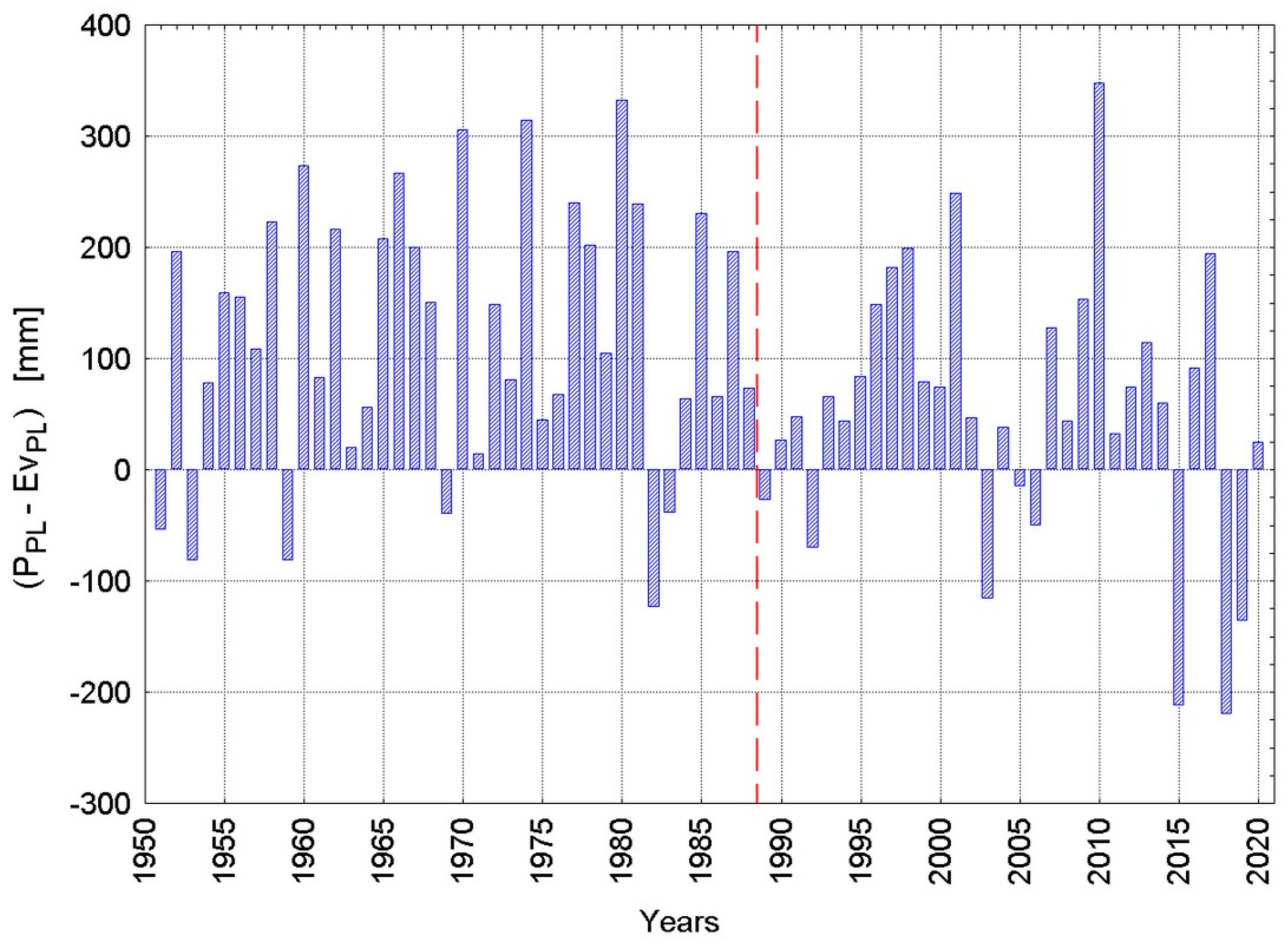
The strong and highly significant increase in field evaporation (EvPL) in 1989–2020, in the face of significant, but practically non-directional changes in annual precipitation totals in the same period, raises the question about the value of the simplified annual water balance (the simplified water balance is considered as the difference between the annual precipitation and the annual evaporation (PPL–EvPL). It is “simplified” in the sense that the non-quantifiable retention is not included) in Poland. The calculated difference between the annual area precipitation totals and the annual area evaporation (PPL–EvPL) shows that in years with a reduced precipitation this balance reached slightly positive values (<100 mm), while in some other years even negative values (Figure 7). While the difference in the number of years with the negative water balance in both sub-periods is not significant (6 and 8 years, respectively), the fundamental change occurs in the distribution of the number of years with specific ranges of the water balance. In the first sub-period (1951–1988) there were 12 years, in which the excess of precipitation over the evaporation per year exceeded 200 mm, while in the second sub-period (1989–2020) there were only 2 years (Figure 5). Moreover, there are clear differences between these sub-periods in terms of the number of years, in which the simplified positive water balance was between 0 and 100 m (11 and 15 years, respectively).
These and other, not discussed here, differences in the distribution of difference between the annual area precipitation and the annual area evaporation (Figure 6A) result in statistically significant differences between the water balance in the two sub-periods (Figure 6B). The balance changed toward a decrease in its positive values in the sub-period following the climate change (in 1951–1988: Lower quartile 56.6 mm, upper quartile 215.8 mm, in 1989–2020: Lower quartile 24.5 mm, upper quartile 114.6 mm), and a strong increase in its amplitude, mainly due to the deepening of the minimum.
This allows us to conclude that along with the climate change that occurred in 1987–1989, despite the lack of statistically significant changes in the course of annual precipitation totals, a statistically significant change in the simplified water balance also took place. The reason for these changes is the strong increase in 1988 in evaporation losses.
5. Number of Days with Low Flows (NDLF) on Polish Rivers
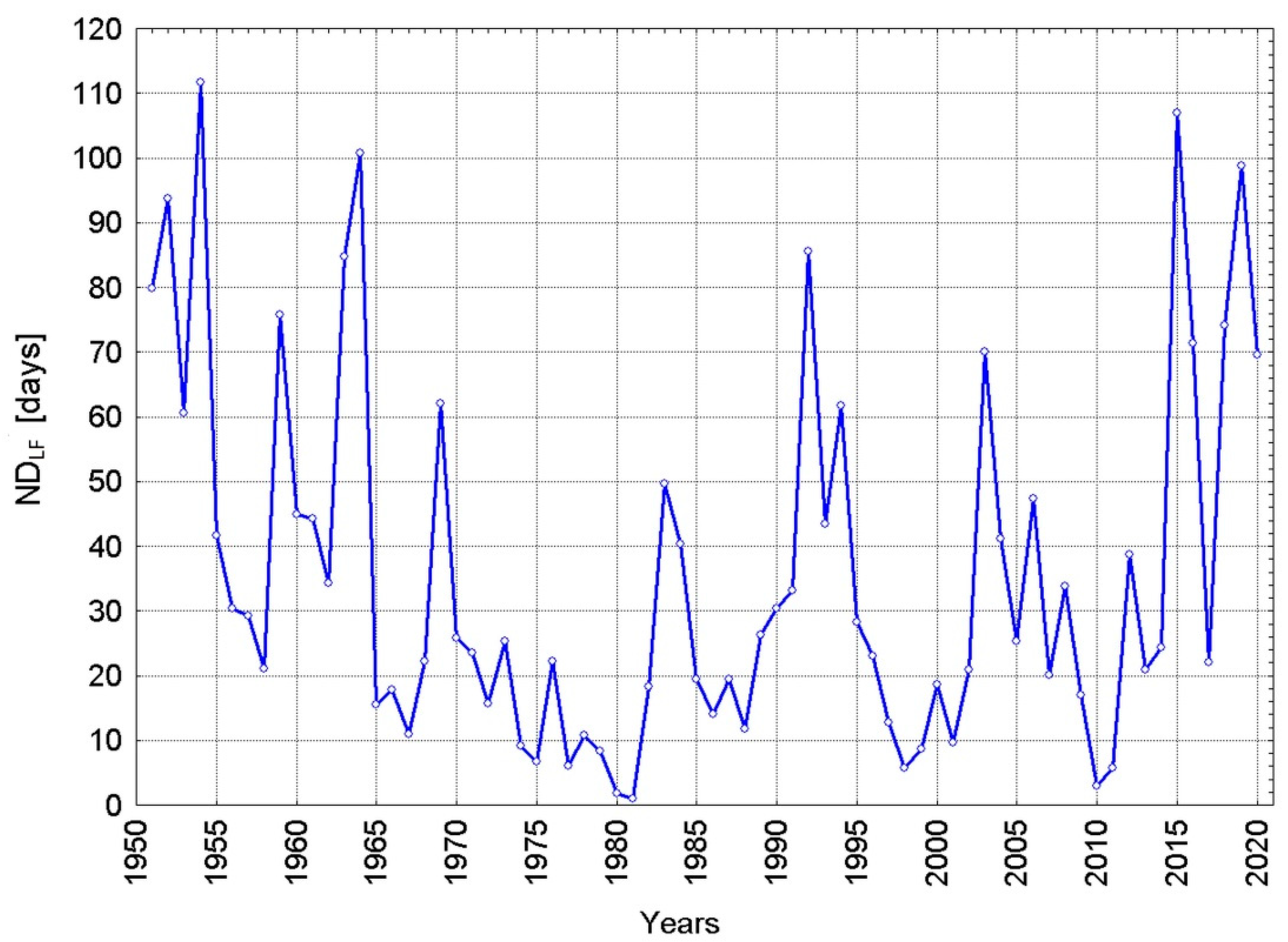
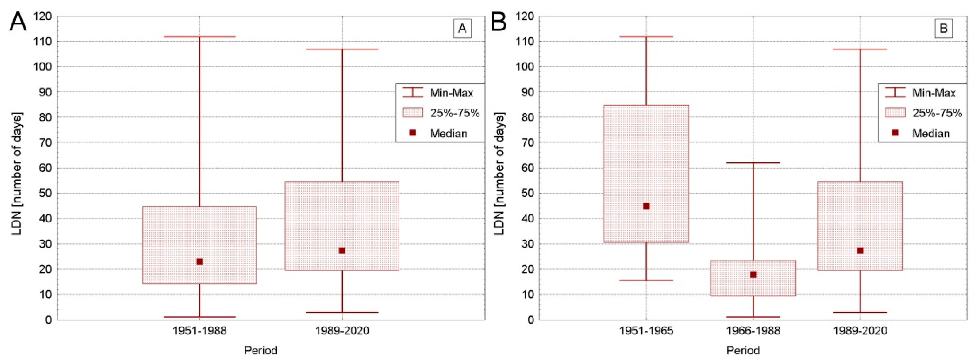
The variability of the annual mean area number of days with low flows in Poland (NDLF) in the multi-annual period 1951–2020 is significant and ranges from one (minimum) to 112 days (maximum), with an average of 35.8 days (standard deviation: σ = 28.5) and a median of 25.3 days. The distribution of NDLF is different from normal, the time series is dominated by years, in which NDLF is within the range of 1–20 days (24 cases) and 21–40 days (22 cases), which in total accounts for ~65.7% of the analyzed 70 years. Only three cases (~4.3%) are in the highest range of distribution (>100 days). The course of area number of days with low flows in the multi-annual period 1951–2020 is shown in Figure 8.
In the course of NDLF, there are usually short periods (from one to several years) in which the number of days with low flows are greater than the average, separated by periods of various lengths, in which the NDLF per year is lower than the average. There was an increased frequency of higher NDLF values at the beginning and end of the analyzed data series. There is a weak (−0.11 (±0.17) and insignificant (p = 0.501) negative trend in the NDLF series.
However, the separation of the NDLF series into two parts, corresponding to the sub-period before climate change and the increased water balance (1951–1988) and the sub-period after climate change and the reduced water balance (Figure 9A), reveals some differences in the distribution of the NDLF values in these sub-periods, and also a slight increase in the NDLF range between the lower and upper quartiles; however, these differences are negligible. Testing of differences between the mean NDLF in both sub-periods indicate that these differences are statistically insignificant. This is surprising, since if the NDLF series is divided in accordance with the time intervals between the circulation epochs (Figure 9B), then both the differences in the distributions and the tests of differences between the mean NDLF prove that there is a statistically significant differentiation in the respective circulation epochs.
Therefore, the result of this part of the analysis is at least ambiguous. On the one hand, it shows that the number of days with low flows clearly differs from the change in the circulation epoch E + C into epoch E, in which the differences between the climatic elements influencing the water balance between these epochs are mostly insignificant. On the other hand, it proves that the strong climate change, leading to a clear change in the water balance, is not significantly reflected in the changes in the average area of the number of days with low flows.
The results obtained require further clarification. In order to get in more detail into the structure of NDLF variance and to explain the connections between NDLF at individual water gauges, the set of the NDLF time series was analyzed with the help of the principal component analysis.
5.1. Results of the Principal Component Analysis
The conducted analysis allowed for the detection of 20 principal components with factor values greater than 1.0, i.e., statistically significant, according to the Kaiser criterion. The scree test indicated that the first four main components [43] were relevant for the analysis, explaining 62.79% of the total variance of the set of analyzed variables (Table 1).
The time series of the factor values of each principal component created eigenvectors, which were then analyzed in terms of their physical meaning. The analysis shows that the first eigenvector (1 EV) is a series of standardized anomalies (deviations from the average of 140 water gauges) in NDLF per year. It explains less than half of the total variance of the set, i.e., 41.4% of the total variance included in the time series of NDLF recorded at 140 water gauges. The physical sense of the second eigenvector (2 EV) is the difference in the response of a certain part of the catchment to changes in water feeding in relation to 1 EV. As it can be concluded from the analysis of the distribution of points on the common areas of individual factor loads, the third and fourth eigenvectors (and the remaining ones, up to 10, not discussed in this paper) present the characteristics of regional differentiation of individual catchment groups, which are the cause of more or less distinct differences in relation to the area average.
The analysis of the eigenvector relationships between five area climatic elements (precipitation—PPL, temperature—TPL, relative humidity—fPL, general cloudiness—NPL, sunshine duration—SDPL) and the annual area evaporation (EvPL) and two large-scale climate indicators, i.e., the winter (DJFM) Hurrell NAO index (PC-based) and the DG3L index, that inform about the intensity of thermohaline circulation in the North Atlantic, allowed for the clarification of a number of issues related to the shaping of the variance structure of NDLF. The results of this analysis are presented in Table 2.
Both the first and second eigenvector with the same strength are positively related to the annual evaporation. The greater it is, the greater the likelihood of low flow. The first eigenvector (1 EV) is negatively related to the annual precipitation totals, general cloudiness, and relative humidity, while positively to sunshine duration. The greater the values of precipitation, cloudiness, and relative humidity, the lower the likelihood of low flows, the greater the sunshine duration, the greater the losses on evaporation, and the greater the likelihood of low flow. It should be noted that 1 EV is not significantly related to temperature. Among the large-scale climate indicators, 1 EV is significantly related only to the DG3L index, which reflects the impact of changes in the thermal state of the North Atlantic on the climate of Poland, but it is not significantly related to the winter NAO index.
The second eigenvector (2 EV) shows almost no relationship with the annual precipitation and general cloudiness. It is strongly and positively related to air temperature and, stronger than 1 EV, to sunshine duration, while weaker to relative humidity. It is highly significantly related to the winter NAO index, which by regulating the duration of snow cover [44,45,46], with a negative sign, has a strong impact on river flows in some parts of Poland [47,48,49,50,51,52], and with a positive sign on the size of winter field evaporation [42,53]. The 2 EV is slightly less than 1 EV related to the DG3L index, which in Poland regulates, among others, the frequency of droughts and, to a lesser extent, the long-term variability of annual river flows [54,55]. Therefore, the variability of 2 EV does not involve the main factor on the “revenue” side of the water balance, i.e., precipitation, but only the factors determining the size of the balance losses.
This allows us to conclude that the variability of 1 and 2 EV is strongly, albeit in different ways, related to the variability of climatic conditions, including variability of the large-scale circulation conditions, and these factors jointly control their variability.
The last eigenvector showing the influence of large-scale circulation indices is 3 EV, which shows the relationship with NAO. In the case of subsequent eigenvectors—4 EV and following—the large-scale influences become negligible, and the relationships with the elements of area climate usually lose their significance, as well.
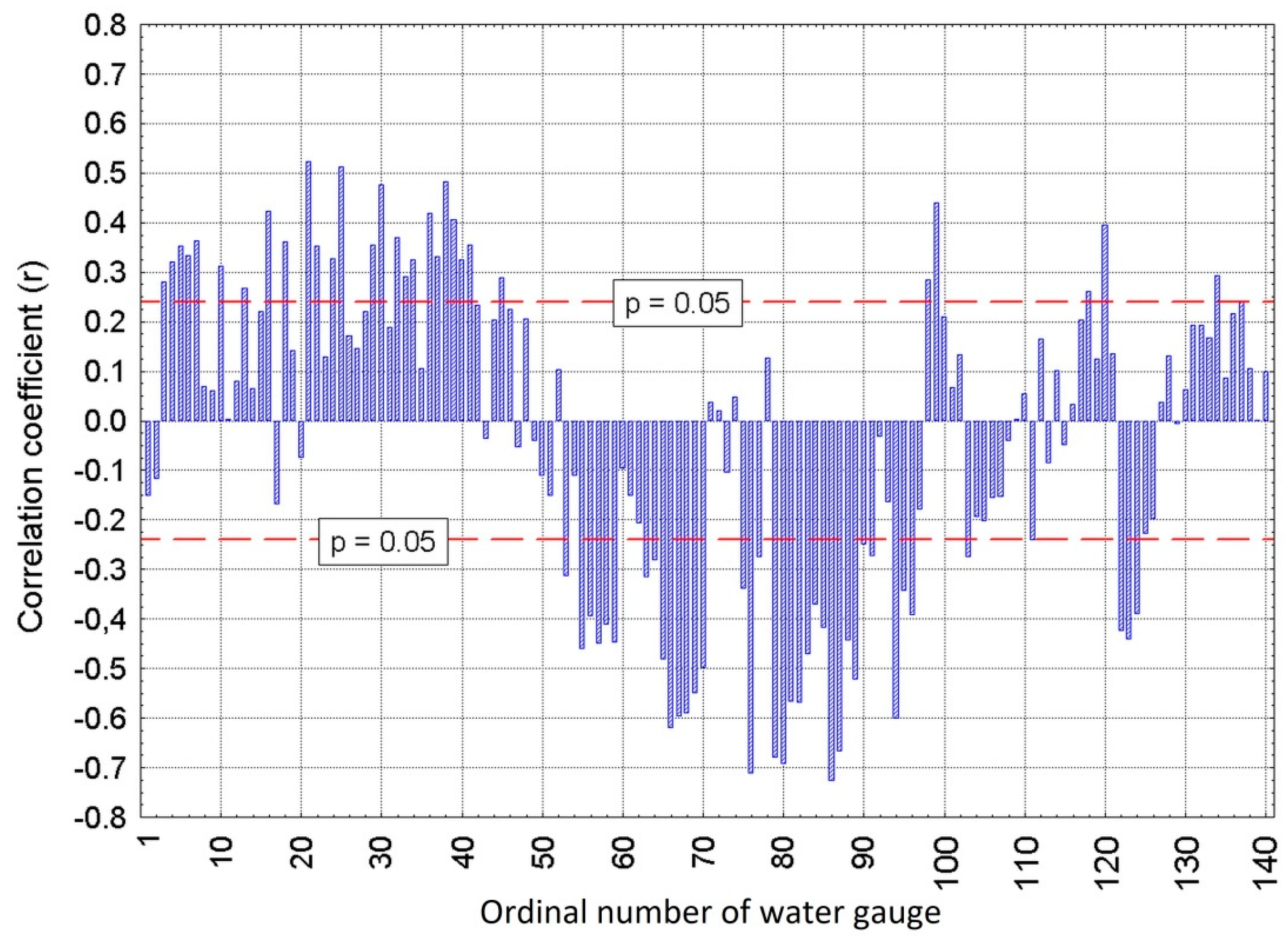
While the first eigenvector is positively correlated with all 140 series of NDLF recorded at individual water gauges (although not significantly in every case), the second and subsequent eigenvectors change their signs in correlation with the individual series of specific groups of water gauges and/or individual water gauges. As the sequence number of the eigenvector increases, the degree of fragmentation of the plot increases, dividing it into sections with positive and negative values of the correlation coefficient (Figure 10). As the water gauges identifiers (ordinal numbers) are arranged geographically according to the location of the catchment area, it clearly indicates the increasing regional and local factors in shaping the diversity of the whole set in relation to the mean, along with the increase in the eigenvector sequence number and its decrease in its importance in explaining the total variance of the set.
To date, it can be assumed that the effect of the not considered factor of the regional differentiation, proves that the statistical analysis of the NDLF relationship with climatic elements, treated as uniform on the country (Poland) scale, does not detect statistically significant changes in NDLF that occur along with the change in climatic conditions (see Figure 9A and Figure 9B). This requires further analysis of the spatial distribution of changes in NDLF at individual water gauges, considered in a function of time.
5.2. Spatial Analysis of the Relationship between the Number of Days with Low Flows (NDLF) and Changes in Climatic Conditions
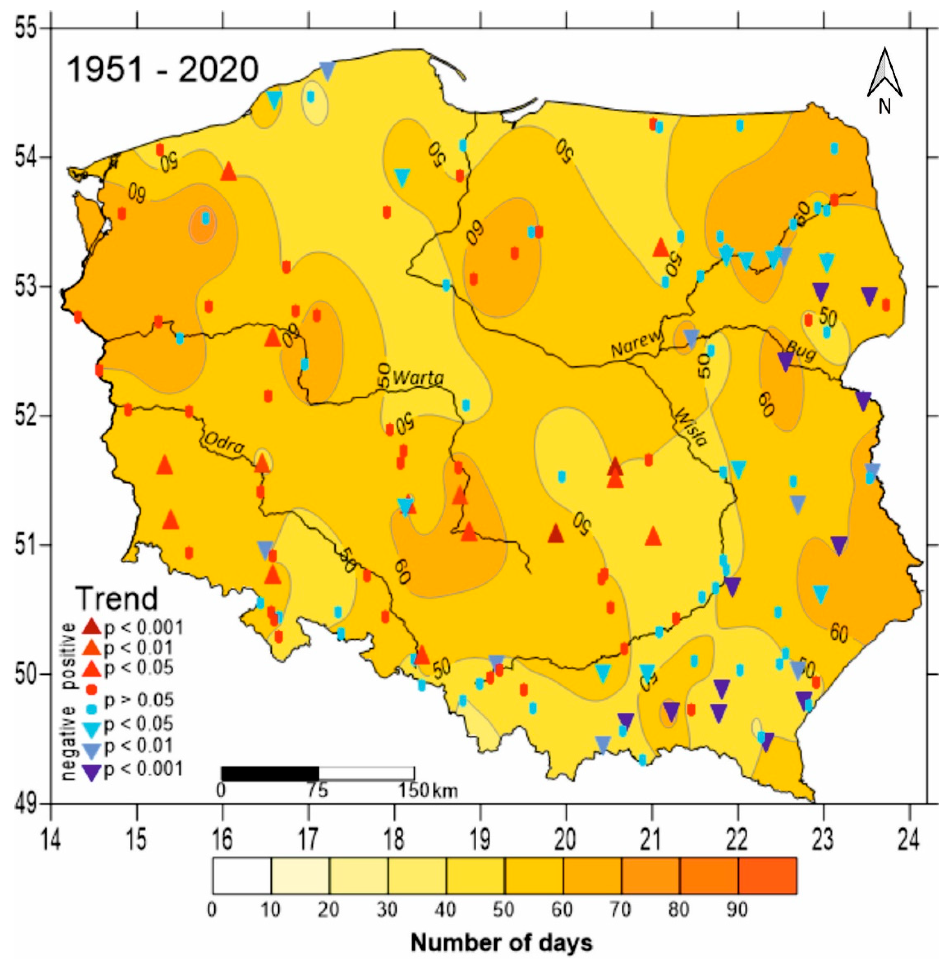
The spatial analysis of the relationship was carried out with the help of the cartographic method. For this purpose, the time series of NDLF from all 140 water gauges with their strictly defined geographical location was investigated. The spatial distribution of the areas through which the flowing rivers have a certain average NDLF per year in Poland in the multi-annual period 1951–2020 is presented in Figure 11.
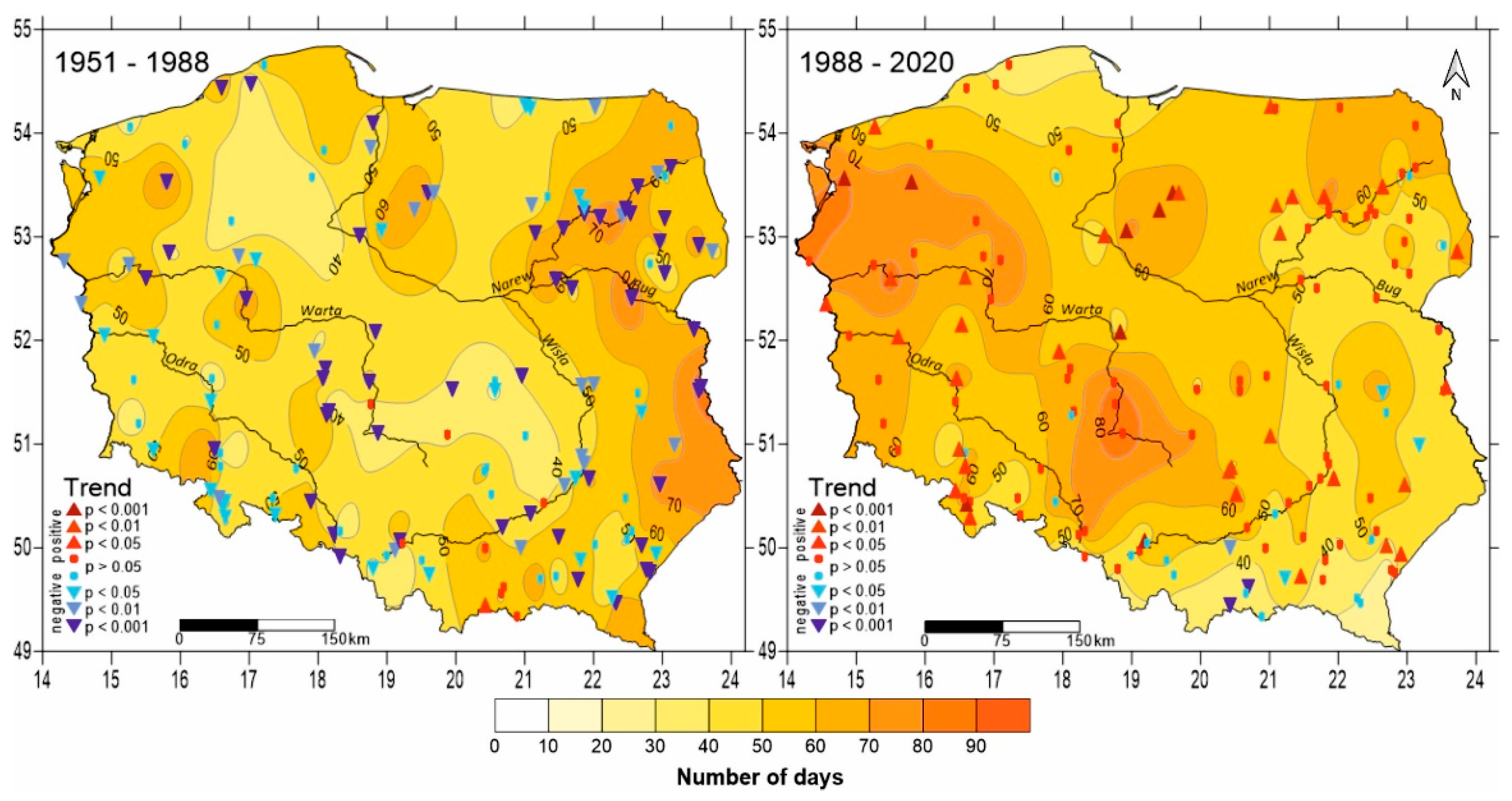
The spatial distribution of NDLF shows quite significant differentiation, creating bands of increasing and decreasing values with the NW–SE course. The increasing number of NDLF is reflected in a kind of “centers” (>60 days a year) marking the axes of these bands. The first band extends from the area of Western Pomerania, through Greater Poland, the Kraków-Częstochowa Upland, to the upper reaches of the Vistula River. The second one stretches from the southern end of the Kashubian Lake District (Kociewie), through the Chełmno and Dobrzyń Land to the eastern part of the Lublin Upland. The third band can be distinguished in the eastern part of the Masurian Lake District and the Suwałki Lake District, and is most likely a part of a longer zone, the continuation of which is located beyond the country borders. The studied trends of changes in NDLF in 1951–2020 (Figure 11) show, despite their mosaic distribution, mostly downward tendencies in the north-eastern and eastern part of Poland, and mostly upward tendencies in its western and south-western parts. The spatial distribution of NDLF obtained for the respective sub-periods—before the climate change (1951–1988) and after it (1988–2020)—proves that in the whole analyzed multi-annual period 1951–2020 they form two different patterns (Figure 12). There was a clear change in the spatial distribution of the areas of increased frequency of NDLF between these sub-periods.
In 1951–1988, the areas with the highest NDLF included rivers located in the eastern part of Poland: From the eastern part of the Masurian Lake District to the southern edge of the Lublin region. In that area, the average NDLF per year exceeded 50 days, and in its relatively large parts, it exceeded 70 days. At the same time, in the western and south-western parts of Poland, there were only single rivers, on which NDLF exceeded 50 days per year, with the maximum >60 days on the Drawa River and the middle Warta River. In the rest of the country, the average NDLF was within the range of 40–50 days per year, while in quite large areas (e.g., central Pomerania, the zone from the upper Warta to the Vistula in the Nida-Połaniec estuary) it was less than 40 days. In this period, negative trends in Poland dominated, most of which were statistically highly significant.
Along with the climate change an abrupt change in the spatial distribution of days with low flows in Poland can be concluded. In 1988–2020, areas with the maximum NDLF were located in western and south-western Poland (Figure 11); in the lower reaches of the Odra River and in the upper reaches of the Warta River, the average NDLF exceeded 80 days per year. On almost all rivers of Central and Eastern Poland, NDLF was greater than 50 days per year. In that period, positive trends in NDLF prevailed, with positive trends of the highest significance (p < 0.001) on rivers located in Western Pomerania, in the upper reaches of the Warta River and on the Drwęca River in the Vistula River basin. Negative trends in NDLF in more continuous areas were detected only on the Carpathian tributaries of the upper Vistula River basin and on the middle and lower Wieprz River in the Lublin region.
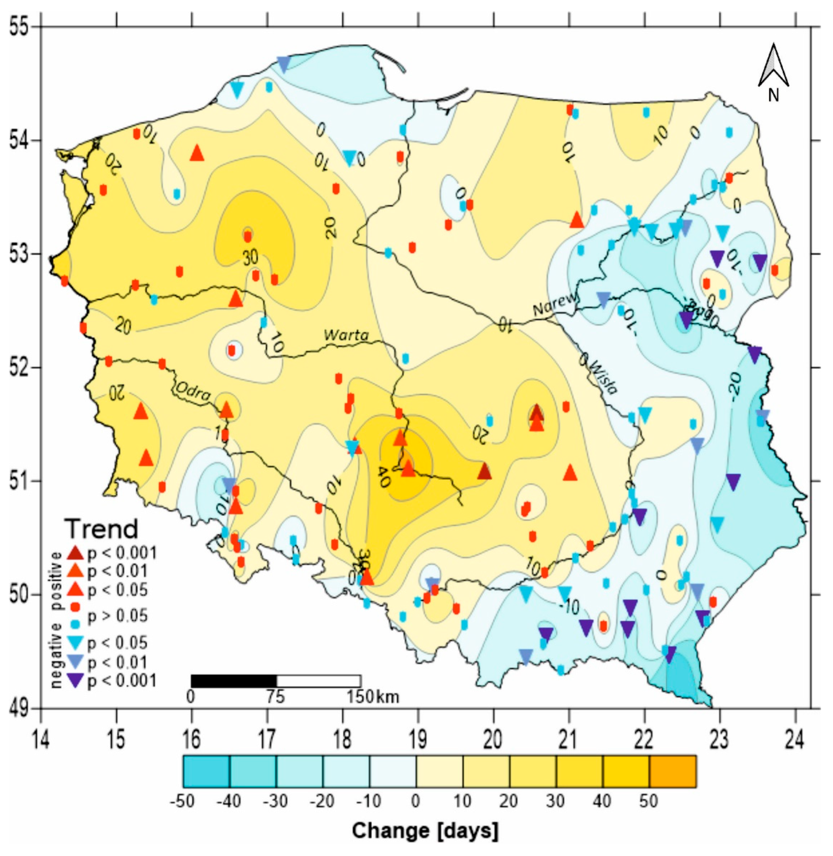
The calculated difference between the average NDLF per year between the sub-period after climate change (1988–2020) and the sub-period before it (1951–1988) (Figure 13) showed that NDLF increased in approximately 2/3 of the area of Poland. The strongest increase took place on the upper Noteć and Warta rivers, where the average NDLF increased by over 30 days.
Continuous areas, in which NDLF decreased, include rivers located in the eastern part of the Vistula River basin, from the Narew River in the northeast to the Raba River, which is a Carpathian tributary of the upper Vistula.
Generally, the analysis of the spatial distribution of NDLF clearly shows that along with the climate change and the change in the water balance in Poland, abrupt changes occurred both in the number of days with low flows and in the spatial distribution of their occurrence (Figure 12 and Figure 13).
6. Discussion
Comparing the results of the cartographic and statistical analyses allows for explaining the reasons why the statistical analysis did not detect statistically significant changes in NDLF in Poland. This analysis was based on a series of averaged values of NDLF for all 140 water gauges. In a situation where during the period of increasing evaporation and decreasing water balance (1988–2020), the changes were multi-directional—in a part of the analyzed area NDLF was increasing and in another part decreasing. With area averaging, opposing trends were mutually compensated and the obtained value of the area average could not properly characterize the spatially diversified course of the studied process.
The main results of the conducted analyses indicate that the observed climate change consisted of a sudden increase in sunshine duration and air temperature, a decrease in relative humidity, leading to an equally strong increase in field evaporation (Figure 7A). In the conditions of significant variability of the annual precipitation totals, this resulted in negative changes in the water balance (Figure 6 and Figure 7B). This, in turn, caused a change in the structure of river flow in Poland (Figure 12 and Figure 13). Along with the decrease in the water balance, NDLF (below Q10) increased in most areas of Poland. Determining the significance level of this increase requires more detailed research, and for this purpose a comparison of differences between the means seems to be more appropriate than the analysis of linear trends.
The greatest increase in NDLF in 1988–2020 was concluded on rivers in western and south-western Poland, while in the same sub-period the number of these days in eastern Poland decreased compared to the preceding sub-period (1951–1988).
The reason for the change in the values of climatic elements that led to climate change was the change in macro-circulation conditions—the transition from the circulation epoch E + C into epoch E, and then from the circulation epoch E into epoch W. Along with the transition from the circulation epoch E into epoch W, not only the values of climatic elements changed, but also the weather structure over Poland was modified. The structure of weather over a given area is determined by the frequency of occurrence of upper ridges and upper troughs (500 hPa) above it [56,57]. To the east of the axis of the upper ridge in the lower troposphere (850–1000 hPa) low-mobility anti-cyclones are formed, and on the border of the eastern part of the upper trough and the western part of the upper ridge cyclones are formed, which then travel toward the top of the wave and then, entering the cool air of the upper trough, they fill up. The anti-cyclonal weather is associated with the occurrence of anti-cyclones over a given area. This is the intra-mass weather characterized by increased sunshine duration and air temperature, reduced cloudiness, and decreased precipitation. The occurrence of the cyclonic system (low) is related to the occurrence of a group of cyclonic weather over a given area. In addition to the intra-mass weather is the frontal weather, characterized by high cloudiness, long-term precipitation, high humidity, very limited sunshine duration, and lower air temperature in the warm half-year.
The Wangengejm-Girs macro-types are nothing but long waves in the mid-troposphere. The macro-type W is characterized by a long wavelength (wavenumber 4), with the upper ridge “stretched” from the eastern North Atlantic to Central Europe, the axis of which is most often located over Western Europe (~5° W–5° E). The macro-type E represents a large-amplitude wave with an upper trough over the eastern North Atlantic and Western Europe and an upper ridge, the axis of which is located over the central part of European Russia (~35°–45° E). When this macro-type occurs, the border between the upper trough and the upper ridge is most often situated between 10° and 20° E [27,37], i.e., above Poland. This factor explains the changes in the spatial distribution of NDLF observed at the same time over Poland (Figure 12 and Figure 13). In 1951–1988, due to the stronger or weaker dominance of the frequency of macro-type E, the eastern part of Poland was more often under the influence of the western edge of the anti-cyclones (highs) from Russia than its western part. Therefore, the frequency of occurrence of water shortages, and thus the occurrence of low flows, was greater over eastern than western Poland, which was located in the zone of an increased frequency of cyclonic weather.
With the transition into the circulation epoch W, there was a significant increase in the frequency of occurrence of the upper ridge axis over Western Europe (~5° W–5° E). Therefore, Poland was more frequently situated on the eastern extremities of the anti-cyclones located above western Europe or the eastern periphery of the vast ridge of the Azores High. The increase in the frequency of the anti-cyclonal weather in this situation was significantly more pronounced over the western than eastern Poland, becoming the cause of a significant increase in the part of “losses” of the water balance and the frequency of low flows in the western part of Poland.
Herein, the expressed assessments of the role of the macro-type W in shaping NDLF—and more generally—the relationship between the reduced runoff of Polish rivers and the increase in the frequency of macro-type W, is contradictory to the opinion expressed by [58], who based on the data from 1901–1965, found that the flows of Polish rivers increased with the increase in the frequency of macro-type W according to the Wangengejm-Girs classification, and the change in the frequency of the macro-type was conditioned by changes in the solar cycles (the Wolf numbers). Studies on the frequency of macro-types of the mid-tropospheric circulation did not confirm (e.g., [27]) the relationship between changes in the frequency of macro-types and changes in the number of sunspots, or more generally—the relationship between changes in the circulation epochs and the 11–13-year cycle of the solar changes. The quality of the initial data (on the frequency of macro-types) and the method of their integration carried out by [58], which were the means calculated for each of the solar cycles, is questionable. Recent studies (e.g., [54,55] as well as this research) have proved that with the increase in the frequency of macro-type W, the flows of Polish rivers do not increase, but decrease.
7. Conclusions
In this study, the daily discharges observed at 140 river gauges on 83 rivers and the series of annual air temperature (T), annual precipitation totals (P), annual values of general cloudiness (N, 1/8), and annual values of relative humidity (f, %) were analyzed. The values of the above-mentioned climatic elements constituted the area averages of 28 stations relatively evenly distributed in Poland. The datasets were used to determine the change in climatic conditions and the duration and trend of changes in the number of days with low flows in the multi-annual period 1951–2020 and in two sub-periods: Before climate change (1951–1988) and after it (1988–2020).
The following conclusions can be drawn based on the results obtained:
- (1)
- In 1987–1989, there was an abrupt change in climatic conditions in Poland.
- (2)
- Climate change in Poland was caused by macro-circulation conditions, controlled by changes in the intensity of thermohaline circulation in the North Atlantic (NA THC).
- (3)
- Climate change consisted of an abrupt increase in sunshine duration and air temperature, and a decrease in relative humidity after 1988. Along with the lack of changes in precipitation totals, characterized by a strong yearly variability, and an increase in field evaporation, it led to noticeable changes in the water balance.
- (4)
- In 1951–2020, the average number of NDFL days was from 30 to 70, with the dominance of upward trends on rivers in central and western Poland and negative trends on the southern and eastern tributaries of the Vistula River.
- (5)
- After climate change in 1989–2020 there was a significant increase in NDFL (even by 1 month) detected in about 2/3 of the area of Poland (in the central and western parts of the country).
- (6)
- With the change in the NA THC phase and the macro-circulation conditions, there was also a change in the spatial distribution of areas drained by rivers with increased NDFL. In 1951–1988, these included the eastern parts of Poland, while after the climate change (1989–2020)—its western and south-western parts.
Author Contributions
Conceptualization, D.W., A.A.M. and A.S.; methodology, D.W., A.A.M. and A.S.; software, D.W., A.A.M., L.S. and A.S.; validation, D.W., A.A.M. and A.S.; formal analysis, D.W., A.A.M. and A.S.; investigation and data curation, D.W., A.A.M. and A.S.; writing—original draft preparation, D.W., A.A.M., L.S. and A.S.; writing—review and editing, L.S.; visualization, D.W., A.A.M. and A.S.; supervision, D.W. and L.S. All authors have read and agreed to the published version of the manuscript.
Funding
The research was carried out under the internal research grant (internal faculty research grant) at the Faculty of Geographical and Geological Sciences of Adam Mickiewicz University in Poznań, Poland.
Institutional Review Board Statement
Not applicable.
Informed Consent Statement
Not applicable.
Data Availability Statement
The data presented in this study are available on request from the corresponding author.
Acknowledgments
We thank the editor and reviewers for their comments and suggestions, which have significantly helped us to improve the manuscript.
Conflicts of Interest
The authors declare no conflict of interest.
Appendix A

Table A1.
Basic data on the studied rivers.
| No. | River | Water Gauge | Longitude (°E) | Latitude (°N) | Catchment Area (km2) | Runoff Depth [mm] | River Regime * |
|---|---|---|---|---|---|---|---|
| 1 | Odra | Chałupki | 18.33 | 49.92 | 4666 | 282.4 | 4 |
| 2 | Odra | Racibórz-Miedonia | 18.23 | 50.12 | 6744 | 300.8 | 4 |
| 3 | Odra | Ścinawa | 16.44 | 51.41 | 29,584 | 188.9 | 4 |
| 4 | Odra | Cigacice | 15.61 | 52.03 | 40,106 | 170.6 | 2 |
| 5 | Odra | Połęcko | 14.89 | 52.05 | 47,370 | 167.1 | 2 |
| 6 | Odra | Słubice | 14.56 | 52.35 | 53,600 | 174.2 | 2 |
| 7 | Odra | Gozdowice | 14.32 | 52.76 | 109,729 | 146.9 | 2 |
| 8 | Sumina | Nędza | 18.31 | 50.16 | 94.4 | 191.3 | 4 |
| 9 | Biała | Dobra | 17.90 | 50.45 | 353 | 99.4 | 4 |
| 10 | Nysa Kłodzka | Bystrzyca Kłodzka | 16.65 | 50.29 | 260 | 466.7 | 4 |
| 11 | Nysa Kłodzka | Kłodzko | 16.66 | 50.44 | 1084 | 364.9 | 4 |
| 12 | Nysa Kłodzka | Nysa | 17.34 | 50.48 | 3276 | 278.6 | 4 |
| 13 | Nysa Kłodzka | Skorogoszcz | 17.67 | 50.76 | 4514 | 249.8 | 4 |
| 14 | Bystrzyca Dusznicka | Szalejów Dolny | 16.60 | 50.42 | 175 | 378.1 | 2 |
| 15 | Ścinawka | Tłumaczów | 16.44 | 50.55 | 256 | 279.8 | 2 |
| 16 | Ścinawka | Gorzuchów | 16.57 | 50.49 | 511 | 274.8 | 4 |
| 17 | Biała Głuchołaska | Głuchołazy | 17.38 | 50.32 | 283 | 542.0 | 4 |
| 18 | Bystrzyca | Krasków | 16.58 | 50.92 | 683 | 205.9 | 4 |
| 19 | Piława | Mościsko | 16.58 | 50.78 | 291 | 172.6 | 4 |
| 20 | Strzegomka | Łażany | 16.49 | 50.95 | 356 | 198.0 | 4 |
| 21 | Barycz | Osetno | 16.46 | 51.63 | 4579 | 101.6 | 3 |
| 22 | Bóbr | Żagań | 15.32 | 51.62 | 4254 | 275.8 | 4 |
| 23 | Kamienica | Barcinek | 15.60 | 50.94 | 97.2 | 389.7 | 2 |
| 24 | Kwisa | Nowogrodziec | 15.40 | 51.20 | 736 | 306.9 | 4 |
| 25 | Warta | Działoszyn | 18.87 | 51.11 | 4088 | 185.8 | 2 |
| 26 | Warta | Sieradz | 18.74 | 51.60 | 8140 | 171.3 | 2 |
| 27 | Warta | Poznań | 16.95 | 52.40 | 25,126 | 124.5 | 2 |
| 28 | Warta | Skwierzyna | 15.50 | 52.60 | 31,268 | 123.4 | 2 |
| 29 | Warta | Gorzów Wielkopolski | 15.25 | 52.73 | 52,186 | 124.4 | 2 |
| 30 | Oleśnica | Niechmirów | 18.76 | 51.39 | 592 | 126.7 | 3 |
| 31 | Ner | Dąbie | 18.82 | 52.08 | 1712 | 181.6 | 2 |
| 32 | Prosna | Mirków | 18.16 | 51.32 | 1255 | 126.0 | 2 |
| 33 | Prosna | Piwonice | 18.11 | 51.73 | 2938 | 119.2 | 2 |
| 34 | Prosna | Bogusław | 17.95 | 51.90 | 4304 | 114.3 | 2 |
| 35 | Niesób | Kuźnica Skakawska | 18.13 | 51.28 | 246 | 123.8 | 3 |
| 36 | Ołobok | Ołobok | 18.07 | 51.64 | 447 | 110.7 | 3 |
| 37 | Mogilnica | Konojad | 16.53 | 52.15 | 663 | 77.3 | 3 |
| 38 | Wełna | Pruśce | 17.10 | 52.77 | 1130 | 92.5 | 3 |
| 39 | Flinta | Ryczywół | 16.84 | 52.82 | 276 | 74.1 | 3 |
| 40 | Sama | Szamotuły | 16.58 | 52.61 | 395 | 83.4 | 3 |
| 41 | Noteć | Nowe Drezdenko | 15.84 | 52.85 | 15,970 | 143.2 | 2 |
| 42 | Gwda | Piła | 16.74 | 53.15 | 4704 | 180.0 | 1 |
| 43 | Drawa | Drawsko Pomorskie | 15.81 | 53.53 | 609 | 209.2 | 2 |
| 44 | Ina | Goleniów | 14.83 | 53.56 | 2163 | 185.5 | 2 |
| 45 | Rega | Trzebiatów | 15.26 | 54.06 | 2628 | 239.4 | 2 |
| 46 | Parsęta | Tychówko | 16.07 | 53.90 | 896 | 289.1 | 2 |
| 47 | Wieprza | Stary Kraków | 16.61 | 54.44 | 1519 | 327.0 | 1 |
| 48 | Słupia | Słupsk | 17.03 | 54.47 | 1450 | 338.5 | 1 |
| 49 | Łupawa | Smołdzino | 17.21 | 54.66 | 805 | 325.7 | 1 |
| 50 | Wisła | Skoczów | 18.79 | 49.80 | 297 | 641.0 | 4 |
| 51 | Wisła | Goczałkowice | 18.99 | 49.93 | 738 | 381.0 | 5 |
| 52 | Wisła | Jawiszowice | 19.12 | 49.97 | 971 | 426.1 | 5 |
| 53 | Wisła | Bieruń Nowy | 19.19 | 50.06 | 1748 | 381.8 | 4 |
| 54 | Wisła | Jagodniki | 20.68 | 50.20 | 12,058 | 334.4 | 4 |
| 55 | Wisła | Szczucin | 21.08 | 50.33 | 23,901 | 307.4 | 4 |
| 56 | Wisła | Sandomierz | 21.75 | 50.67 | 31,846 | 284.8 | 4 |
| 57 | Wisła | Zawichost | 21.86 | 50.81 | 50,732 | 261.9 | 4 |
| 58 | Wisła | Annopol | 21.83 | 50.89 | 51,518 | 261.8 | 4 |
| 59 | Wisła | Dęblin | 21.83 | 51.56 | 68,234 | 227.9 | 4 |
| 60 | Wisła | Toruń | 18.61 | 53.01 | 181,033 | 167.5 | 2 |
| 61 | Wisła | Tczew | 18.80 | 54.10 | 194,376 | 167.3 | 2 |
| 62 | Soła | Oświęcim | 19.22 | 50.04 | 1386 | 473.1 | 4 |
| 63 | Skawa | Sucha Beskidzka | 19.61 | 49.74 | 468 | 507.9 | 4 |
| 64 | Skawa | Wadowice | 19.51 | 49.88 | 836 | 465.0 | 4 |
| 65 | Raba | Proszówki | 20.43 | 50.00 | 1470 | 356.6 | 4 |
| 66 | Dunajec | Krościenko | 20.43 | 49.44 | 1580 | 634.9 | 5 |
| 67 | Dunajec | Nowy Sącz | 20.69 | 49.63 | 4341 | 472.8 | 4 |
| 68 | Poprad | Muszyna | 20.89 | 49.34 | 1514 | 365.9 | 4 |
| 69 | Poprad | Stary Sącz | 20.66 | 49.57 | 2071 | 380.5 | 4 |
| 70 | Biała | Koszyce Wielkie | 20.95 | 50.00 | 957 | 290.5 | 4 |
| 71 | Nida | Brzegi | 20.41 | 50.74 | 2259 | 177.1 | 2 |
| 72 | Nida | Pińczów | 20.52 | 50.51 | 3352 | 168.2 | 2 |
| 73 | Czarna Nida | Tokarnia | 20.45 | 50.77 | 1216 | 171.4 | 2 |
| 74 | Czarna | Połaniec | 21.28 | 50.43 | 1354 | 149.2 | 3 |
| 75 | Wisłoka | Żółków | 21.46 | 49.73 | 581 | 384.7 | 4 |
| 76 | Ropa | Klęczany | 21.22 | 49.70 | 483 | 406.9 | 4 |
| 77 | Brzeźnica | Brzeźnica | 21.49 | 50.11 | 484 | 212.5 | 4 |
| 78 | Koprzywianka | Koprzywnica | 21.57 | 50.60 | 502 | 127.1 | 3 |
| 79 | San | Lesko | 22.32 | 49.47 | 1614 | 555.0 | 4 |
| 80 | San | Przemyśl | 22.77 | 49.78 | 3686 | 444.9 | 4 |
| 81 | San | Jarosław | 22.70 | 50.02 | 7041 | 312.7 | 4 |
| 82 | San | Radomyśl | 21.93 | 50.67 | 16,824 | 241.6 | 4 |
| 83 | Osława | Zagórz | 22.27 | 49.51 | 505 | 509.0 | 4 |
| 84 | Wiar | Krówniki | 22.82 | 49.77 | 789 | 252.7 | 4 |
| 85 | Wisznia | Nienowice | 22.92 | 49.94 | 1185 | 178.6 | 4 |
| 86 | Wisłok | Krosno | 21.77 | 49.69 | 596 | 327.8 | 4 |
| 87 | Wisłok | Żarnowa | 21.82 | 49.88 | 1427 | 287.3 | 4 |
| 88 | Wisłok | Rzeszów | 22.02 | 50.04 | 2086 | 263.1 | 4 |
| 89 | Wisłok | Tryńcza | 22.55 | 50.16 | 3516 | 227.7 | 4 |
| 90 | Mleczka | Gorliczyna | 22.49 | 50.08 | 529 | 173.2 | 4 |
| 91 | Tanew | Harasiuki | 22.47 | 50.48 | 2034 | 189.7 | 2 |
| 92 | Kamienna | Wąchock | 21.02 | 51.08 | 476 | 192.7 | 2 |
| 93 | Wieprz | Zwierzyniec | 22.97 | 50.61 | 405 | 160.1 | 1 |
| 94 | Wieprz | Krasnystaw | 23.18 | 50.99 | 3001 | 129.8 | 2 |
| 95 | Wieprz | Lubartów | 22.64 | 51.50 | 6364 | 111.7 | 2 |
| 96 | Wieprz | Kośmin | 22.00 | 51.57 | 10,231 | 113.2 | 2 |
| 97 | Bystrzyca | Sobianowice | 22.69 | 51.30 | 1265 | 125.6 | 2 |
| 98 | Pilica | Przedbórz | 19.88 | 51.09 | 2536 | 185.9 | 2 |
| 99 | Pilica | Nowe Miasto | 20.57 | 51.61 | 6717 | 166.9 | 2 |
| 100 | Pilica | Białobrzegi | 20.95 | 51.66 | 8664 | 160.4 | 2 |
| 101 | Wolbórka | Zawada | 19.94 | 51.53 | 616 | 137.5 | 2 |
| 102 | Drzewiczka | Odrzywół | 20.56 | 51.52 | 1004 | 166.9 | 2 |
| 103 | Narew | Narew | 23.52 | 52.92 | 1978 | 146.0 | 3 |
| 104 | Narew | Suraż | 22.96 | 52.95 | 3376 | 139.5 | 3 |
| 105 | Narew | Strękowa Góra | 22.54 | 53.22 | 7181 | 141.4 | 3 |
| 106 | Narew | Wizna | 22.41 | 53.20 | 14,308 | 148.4 | 3 |
| 107 | Narew | Piątnica-Łomża | 22.09 | 53.19 | 15,296 | 150.9 | 3 |
| 108 | Narew | Nowogród | 21.86 | 53.23 | 20,106 | 152.4 | 3 |
| 109 | Narew | Ostrołęka | 21.56 | 53.08 | 21,862 | 155.8 | 3 |
| 110 | Narewka | Narewka | 23.73 | 52.86 | 590 | 156.9 | 3 |
| 111 | Supraśl | Fasty | 23.03 | 53.18 | 1817 | 153.3 | 2 |
| 112 | Biebrza | Sztabin | 23.12 | 53.67 | 846 | 171.5 | 3 |
| 113 | Biebrza | Dębowo | 22.93 | 53.61 | 2322 | 167.3 | 3 |
| 114 | Biebrza | Osowiec | 22.64 | 53.48 | 4365 | 160.0 | 3 |
| 115 | Biebrza | Burzyn | 22.46 | 53.27 | 6900 | 158.0 | 3 |
| 116 | Brzozówka | Karpowicze | 23.04 | 53.59 | 650 | 154.1 | 3 |
| 117 | Pisa | Ptaki | 21.79 | 53.39 | 3562 | 181.6 | 1 |
| 118 | Pisa | Dobrylas | 21.87 | 53.28 | 4061 | 182.4 | 2 |
| 119 | Rozoga | Myszyniec | 21.34 | 53.39 | 231 | 155.2 | 2 |
| 120 | Omulew | Krukowo | 21.11 | 53.31 | 1265 | 170.0 | 2 |
| 121 | Orzyc | Krasnosielc | 21.15 | 53.04 | 1268 | 142.2 | 2 |
| 122 | Bug | Włodawa | 23.57 | 51.55 | 14,410 | 120.5 | 3 |
| 123 | Bug | Frankopol | 22.56 | 52.41 | 31,336 | 118.1 | 3 |
| 124 | Bug | Wyszków | 21.45 | 52.59 | 39,119 | 122.5 | 3 |
| 125 | Włodawka | Okuninka | 23.52 | 51.52 | 576 | 116.5 | 3 |
| 126 | Krzna | Malowa Góra | 23.47 | 52.10 | 3128 | 108.1 | 3 |
| 127 | Nurzec | Boćki | 23.04 | 52.65 | 556 | 134.0 | 3 |
| 128 | Nurzec | Brańsk | 22.82 | 52.74 | 1227 | 126.8 | 3 |
| 129 | Liwiec | Łochów | 21.68 | 52.51 | 2466 | 134.1 | 3 |
| 130 | Drwęca | Nowe Miasto Lubawskie | 19.59 | 53.42 | 2725 | 188.9 | 2 |
| 131 | Drwęca | Brodnica | 19.40 | 53.26 | 3526 | 192.5 | 2 |
| 132 | Drwęca | Elgiszewo | 18.93 | 53.06 | 4959 | 173.7 | 2 |
| 133 | Wel | Kuligi | 19.69 | 53.43 | 764 | 206.3 | 1 |
| 134 | Brda | Tuchola | 17.90 | 53.57 | 2462 | 248.6 | 1 |
| 135 | Wda | Czarna Woda | 18.09 | 53.84 | 940 | 210.7 | 1 |
| 136 | Wierzyca | Brody Pomorskie | 18.76 | 53.86 | 1544 | 175.0 | 2 |
| 137 | Łyna | Sępopol | 21.01 | 54.27 | 3647 | 211.7 | 2 |
| 138 | Guber | Prosna | 21.09 | 54.23 | 1568 | 171.6 | 2 |
| 139 | Gołdapa | Banie Mazurskie | 22.03 | 54.25 | 548 | 266.9 | 3 |
| 140 | Czarna Hańcza | Czerwony Folwark | 23.12 | 54.07 | 454 | 262.6 | 2 |
References
- Schmuck, A. Outline of Hydrometeorology; Wydawnictwo Naukowe PWN: Wrocław-Warsaw, Poland, 1960; pp. 1–108. (In Polish) [Google Scholar]
- Bac, S. Studies on evaporation of free water surface field, field evaporation and potential evapotranspiration. Zesz. Nauk. WSR We Wrocławiu 1968, 80, Melioracja 13, 7–68. (In Polish) [Google Scholar]
- Kędziora, A. Fundamentals of Agro-Meteorology; Państwowe Wydawnictwo Rolnicze i Leśne: Warsaw, Poland, 1999; pp. 1–364. (In Polish) [Google Scholar]
- Giuntoli, I.; Renard, B.; Vidal, J.-P.; Bard, A. Low flows in France and their relationship to large-scale climate indices. J. Hydrol. 2013, 482, 105–118. [Google Scholar] [CrossRef]
- Shorthouse, C.; Arnell, N. Spatial and temporal variability in European river flows and the North Atlantic Oscillation. In FRIEND 97-Regional Hydrology: Concepts and Models for Sustainable Water Resource Management; IAHS Publ: Wallingford, UK, 1997; Volume 246. [Google Scholar]
- Bouwer, L.M.; Vermaat, J.E.; Aerts, J.C.J.H. Regional sensitivities of mean and peak river discharge to climate variability in Europe. J. Geophys. Res. 2008, 113, D19103. [Google Scholar] [CrossRef]
- Wilby, R.; O’Hare, G.; Barnsley, N. The North Atlantic Oscillation and British Isles climate variability, 1865–1996. Weather 1997, 52, 266–276. [Google Scholar] [CrossRef]
- Kiely, G. Climate change in Ireland from precipitation and streamflow observations. Adv. Water Resour. 1999, 23, 141–151. [Google Scholar] [CrossRef]
- Kingston, D.G.; Hannah, D.M.; Lawler, D.M.; McGregor, G.R. Interactions between Large-Scale Climate and River Flow across the Northern North Atlantic Margin; IAHS-AISH Publ: Havana, Cuba, 2006; pp. 350–355. [Google Scholar]
- Wedgbrow, C.S.; Wilby, R.L.; Fox, H.R.; O’Hare, G. Prospects for seasonal forecasting of summer drought and low river flow anomalies in England and Wales. Int. J. Climatol. 2002, 22, 219–236. [Google Scholar] [CrossRef]
- Stefan, S.; Ghioca, M.; Rimbu, N.; Boroneant, C. Study of meteorological and hydrological drought in southern Romania from observational data. Int. J. Climatol. 2004, 24, 871–881. [Google Scholar] [CrossRef]
- Mager, P.; Kuźnicka, M.; Kępińska-Kasprzak, M.; Farat, R. Changes in the intensity and frequency of occurrence of droughts in Poland (1891–1995). Geogr. Pol. 2000, 73, 41–48. [Google Scholar]
- Łabędzki, L. Estimation of local drought frequency in central Poland using the standardized precipitation index SPI. Irrig. Drain. 2007, 56, 6777. [Google Scholar] [CrossRef]
- Tokarczyk, T. Widely applied indices for drought assessment and Polish application. In Infrastruktura i Ekologia Terenów Wiejskich; Stowarzyszenie Infrastruktura i Ekologia Terenów Wiejskich: Kraków, Poland, 2008; Volume 7, pp. 167–182. (In Polish) [Google Scholar]
- Tokarczyk, T. Low-Water Flows as an Indicator of Hydrological Drought; Instytut Meteorologii i Gospodarki Wodnej: Warsaw, Poland, 2010; pp. 1–164. (In Polish) [Google Scholar]
- Tokarczyk, T. Classification of low flow and hydrological drought for a river basin. Acta Geophys. 2013, 61, 404–421. [Google Scholar] [CrossRef]
- Szalińska, W. Combined analysis of precipitation and water deficit for drought hazard assessment. Hydrol. Sci. J. 2014, 59, 1675–1689. [Google Scholar] [CrossRef]
- Tomaszewski, E.; Kozek, M. Dynamics, Range, and Severity of Hydrological Drought in Poland. In Management of Water Resources in Poland; Zeleňáková, M., Kubiak-Wójcicka, K., Negm, A.M., Eds.; Springer Nature: Cham, Switzerland, 2021. [Google Scholar] [CrossRef]
- Tomaszewski, E.; Kubiak-Wójcicka, K. 2021: Low-Flows in Polish Rivers. In Management of Water Resources in Poland; Zeleňáková, M., Kubiak-Wójcicka, K., Negm, A.M., Eds.; Springer Nature: Cham, Switzerland, 2021. [Google Scholar] [CrossRef]
- Szwed, M.; Karg, G.; Pinskwar, I.; Radziejewski, M.; Graczyk, D.; Kędziora, A.; Kundzewicz, Z.W. Climate change and its effect on agriculture, water resources and human health sectors in Poland. Nat. Hazards Earth Syst. Sci. 2010, 10, 1725–1737. [Google Scholar] [CrossRef]
- Meresa, H.K.; Osuch, M.; Romanowicz, R. Hydro-Meteorological Drought Projections into the 21-st Century for Selected Polish Catchments. Water 2016, 8, 206. [Google Scholar] [CrossRef]
- Instytut Meteorologii i Gospodarki Wodnej–Państwowy Instytut Badawczy. Dane Publiczne. Available online: https://danepubliczne.imgw.pl (accessed on 20 May 2021). (In Polish).
- Bryś, K. Dynamics of Net Radiation Balance of Grass Surface and Bare Soil; Monografie CLXII, Wydawnictwo Uniwersytetu Przyrodniczego we Wrocławiu: Wrocław, Poland, 2013; pp. 1–288. (In Polish) [Google Scholar]
- Matuszko, D. Long-term variability in solar radiation in Krakow based on measurements of sunshine duration. Int. J. Climatol. 2014, 34, 228–234. [Google Scholar] [CrossRef]
- Matuszko, D.; Piotrowicz, K. Relationship between sunshine duration and air temperature on the basis of long-term climatological series in Krakow (1884–2016). Przegląd Geofiz. 2018, 63, 15–29. (In Polish) [Google Scholar]
- Podstawczyńska, A. The solar characteristics of climate of Łódź. Acta Univ. Lodz. Folia Geogr. Phys. 2007, 7, 1–220. (In Polish) [Google Scholar]
- Dimitriev, A.A.; Dubravin, V.F.; Belyazo, V.A. The Atmospheric Processes in the Northern Hemisphere (1891–2018), Their Classification and Use; SUPER Izdatielstvo: Sankt Petersburg, Russia, 2018; pp. 1–305. (In Russian) [Google Scholar]
- Kalnay, E.; Kanamitsu, M.; Kistler, R.; Collins, W.; Deaven, D.; Gandin, L.; Iredell, M.; Saha, S.; White, G.; Woollen, J.; et al. The NCEP/NCAR 40-Year Reanalysis Project. Bull. Am. Meteorol. Soc. 1996, 77, 437–471. [Google Scholar] [CrossRef]
- Okołowicz, W. General Climatology; Wydawnictwo Naukowe PWN: Warsaw, Poland, 1976; pp. 1–422. (In Polish) [Google Scholar]
- Kędziora, A. Water balance of Konin strip mine landscape in changing climatic conditions. Rocz. Glebozn. 2008, 59, 104–118. (In Polish) [Google Scholar]
- Radzka, E. Climatic water balance for the vegetation season (according to Ivanov’s equation) in Central-Eastern Poland. Woda-Środowisko-Obsz. Wiej. 2014, 14, 67–76. (In Polish) [Google Scholar]
- Okoniewska, M.; Szumińska, D. Changes in Potential Evaporation in the Years 1952–2018 in North-Western Poland in Termsof the Impact of Climatic Changes on Hydrological an Hydrochemical Condotions. Water 2020, 12, 877. [Google Scholar] [CrossRef]
- Yevjevich, V. An Objective Approach to Definitions and Investigations of Continental Hydrologic Droughts. Hydrology Papers; Colorado State University: Fort Collins, CO, USA, 1967; pp. 1–25. [Google Scholar]
- Ozga-Zielińska, M.; Brzeziński, J. Applied Hydrology; Wydawnictwo Naukowe PWN: Warsaw, Poland, 1994; pp. 1–323. (In Polish) [Google Scholar]
- Wangengejm, G.Y. Fundamentals of macrocirculation method for long-range weather forecasting for the Arctic. In Trudy; AANII: Leningrad, USSR, 1952; Volume 34, pp. 1–314. (In Russian) [Google Scholar]
- Girs, A.A. On the creation of a single classification of the northern hemisphere. Meteorol. I Gidrol. 1964, 4, 43–47. (In Russian) [Google Scholar]
- Girs, A.A. Long-Term Atmospheric Circulation Variations, and Long-Range Hydrometeorological Forecasts; Girometeoizdat: Leningrad, USSR, 1971; pp. 1–280. (In Russian) [Google Scholar]
- Savichev, A.I.; Mironicheva, N.P.; Cepelev, V.Y. Atmospheric circulation characteristics of the northern hemisphere of the Atlantic-Eurasian sector for last decades. Uchenye Zap. Ross. Gos. Gidrometeorol. Univ. 2015, 39, 120–131. (In Russian) [Google Scholar]
- Degirmendžić, J.; Kożuchowski, K. Circulation epochs based on the Vangengeim-Girs large scale patterns (1891–2010). Acta Univ. Lodz. Folia Geogr. Phys. 2018, 17, 7–13. [Google Scholar] [CrossRef]
- Degirmnedžić, J.; Kożuchowski, K. Variation of macro-circulation forms over the Atlantic-Eurasian temperate zone according to the Vangengeim-Girs classification. Int. J. Climatol. 2019, 39, 4938–4942. [Google Scholar] [CrossRef]
- Monin, A.S. An Introduction to the Theory of Climate; Gidrometoizdat: Leningrad, USSR, 1982; pp. 1–246. (In Russian) [Google Scholar]
- Marsz, A.A.; Styszyńska, A. The Influence of the Sign of NAO Phases during the Winter Period on the Water Balance and the Possibility of Drought Occurrence in the Warm Season in Poland. Ann. Univ. Mariae Curie-Skłodowska 2021, 76, 127–143. [Google Scholar] [CrossRef]
- Hill, T.; Lewicki, P. Statistics: Methods and Applications; StatSoft: Tulsa, OK, USA, 2007. [Google Scholar]
- Bednorz, E. Snow cover in eastern Europe in relation to temperature, precipitation and circulation. Int. J. Climatol. 2004, 24, 591–601. [Google Scholar] [CrossRef]
- Czarnecka, M. Frequency of occurrence and depth of snow cover in Poland. Acta Agrophys. 2012, 19, 501–514. (In Polish) [Google Scholar]
- Tomczyk, A.M. Impact of macro-scale circulation types on the occurrence of snow cover in Europe. Acta Geogr. Sil. 2014, 15, 65–69. (In Polish) [Google Scholar]
- Pociask-Karteczka, J. River Hydrology and the North Atlantic Oscillation: A General Review. AMBIO 2006, 35, 312–314. [Google Scholar] [CrossRef] [PubMed]
- Styszyńska, A.; Tamulewicz, J. Warta river discharges in Poznań and atmospheric circulation in the North Atlantic region. Quaest. Geogr. 2004, 23, 63–81. [Google Scholar]
- Wrzesiński, D. Changes of the hydrological regime of rivers of northern and central Europe in various circulation periods of the North Atlantic Oscillation. Quaest. Geogr. 2005, 24, 97–109. [Google Scholar]
- Wrzesiński, D. Typology of spatial patterns seasonality in European rivers flow regime. Quaest. Geogr. 2008, 27, 87–98. [Google Scholar]
- Wrzesiński, D. Regional differences in the influence of the North Atlantic Oscillation on seasonal river runoff in Poland. Quaest. Geogr. 2011, 30, 127–136. [Google Scholar] [CrossRef]
- Wrzesiński, D.; Paluszkiewicz, R. Spatial differences in the impact of the North Atlantic Oscillation on the flow of rivers in Europe. Hydrol. Res. 2011, 42, 30–39. [Google Scholar] [CrossRef]
- Marsz, A.A.; Styszyńska, A. Intensity of thermohaline Circulation in the North Atlantic and Droughts in Poland. Pr. I Studia Geogr. 2021, 66, 63–88. (In Polish) [Google Scholar] [CrossRef]
- Marsz, A.A.; Styszyńska, A.; Krawczyk, W.E. Long-term fluctuations of annual discharges of the main rivers in Poland and their association with the Northern Atlantic Thermohaline Circulation. Przegląd Geogr. 2016, 88, 295–316. (In Polish) [Google Scholar] [CrossRef]
- Wrzesiński, D.; Marsz, A.A.; Styszyńska, A.; Sobkowiak, L. Effect of the North Atlantic Thermohaline Circulation on Changes in Climatic Conditions and River Flow in Poland. Water 2019, 11, 1662. [Google Scholar] [CrossRef]
- Fortak, H. Meteorology; Deutsche Buch-Gemainschaft: Berlin, Germany; Darmstadt, Germany; Wien, Austria, 1971; pp. 1–287. (In German) [Google Scholar]
- Zvieriev, A.S. Synoptic Meteorology; Gidrometeoizdat: Leningrad, USSR, 1977; pp. 1–711. (In Russian) [Google Scholar]
- Stachý, J. Long-term forecast of the runoff of Polish rivers. In PIH-M Wiadomości Służby Hydrol. i Meteorol; Państwowy Instytut Hydrologiczno-Meteorologiczny: Warsaw, Poland, 1969; Volume 3, pp. 23–34. (In Polish) [Google Scholar]
- Wrzesiński, D. Use of Entropy in the Assessment of Uncertainty of River Runoff Regime in Poland. Acta Geophys. 2016, 64, 1825–1839. [Google Scholar] [CrossRef]
- Wrzesiński, D. Flow Regime Patterns and Their Changes. In Management of Water Resources in Poland; Zeleňáková, M., Kubiak-Wójcicka, K., Negm, A.M., Eds.; Springer Nature: Cham, Switzerland, 2021; pp. 163–180. [Google Scholar] [CrossRef]
Figure 1.
Position of the analyzed water gauges and meteorological stations in Poland.

Figure 2.
The course of the anomaly in the annual frequency of the mid-tropospheric circulation macro-types W, E, and C, according to the Wangengejm-Girs classification, in 1951–2020. Anomalies calculated based on averages from 1951–2000. Boundaries of the circulation epochs are marked with the vertical dashed lines.

Figure 3.
Courses of the annual area air temperature (TPL) (A) and sunshine duration (SDPL) (B) in Poland in 1951–2020. The year 1988, when the courses changed and a positive trend appeared, is marked with the vertical dashed line.
Figure 3.
Courses of the annual area air temperature (TPL) (A) and sunshine duration (SDPL) (B) in Poland in 1951–2020. The year 1988, when the courses changed and a positive trend appeared, is marked with the vertical dashed line.

Figure 4.
Ranges of variability of the annual area air temperature (TPL) (A) and sunshine duration (SDPL) (B) in Poland in sub-periods 1951–1988 and 1989–2020.
Figure 4.
Ranges of variability of the annual area air temperature (TPL) (A) and sunshine duration (SDPL) (B) in Poland in sub-periods 1951–1988 and 1989–2020.

Figure 5.
Course of the annual area precipitation (PPL) in Poland in 1951–2020.

Figure 6.
Ranges of variability of the annual area field evaporation (Ev) (A) and simplified water balance (B) in Poland in sub-periods 1951–1988 and 1989–2020.
Figure 6.
Ranges of variability of the annual area field evaporation (Ev) (A) and simplified water balance (B) in Poland in sub-periods 1951–1988 and 1989–2020.

Figure 7.
Values of the simplified annual area water balance (mm) in 1951–2020. The sub-periods 1951–1988 and 1989–2020 are separated with the vertical dashed line.
Figure 7.
Values of the simplified annual area water balance (mm) in 1951–2020. The sub-periods 1951–1988 and 1989–2020 are separated with the vertical dashed line.

Figure 8.
Course of the average number of days with low flows (NDLF) in Poland in 1951–2020.

Figure 9.
Ranges of variability of the average number of days with low flows (NDLF) in sub-periods before (1951–1988) and after climate change (1989–2020) (A) and in three sub-periods corresponding to different macro-circulation epochs (B).
Figure 9.
Ranges of variability of the average number of days with low flows (NDLF) in sub-periods before (1951–1988) and after climate change (1989–2020) (A) and in three sub-periods corresponding to different macro-circulation epochs (B).

Figure 10.
Correlation coefficients (r) between 2 EV of the set of NDLF and NDLF per year at individual water gauges in Poland in 1951–2020. The lower boundary of statistical significance (p = 0.05) is marked with the dashed line.
Figure 10.
Correlation coefficients (r) between 2 EV of the set of NDLF and NDLF per year at individual water gauges in Poland in 1951–2020. The lower boundary of statistical significance (p = 0.05) is marked with the dashed line.

Figure 11.
Spatial distribution of NDLF and the trends of changes in 1951–2020 with their statistical significance (p).
Figure 11.
Spatial distribution of NDLF and the trends of changes in 1951–2020 with their statistical significance (p).

Figure 12.
Spatial distribution of NDLF and the trends of changes in 1951–1988 and 1988–2020. Explanations as in Figure 11.
Figure 12.
Spatial distribution of NDLF and the trends of changes in 1951–1988 and 1988–2020. Explanations as in Figure 11.

Figure 13.
Spatial distribution of changes in NDLF between 1988–2020 (after climate change) and 1951–1988 (before climate change in 1987–1989) and trends of changes in 1951–2020 with their statistical significance (p).
Figure 13.
Spatial distribution of changes in NDLF between 1988–2020 (after climate change) and 1951–1988 (before climate change in 1987–1989) and trends of changes in 1951–2020 with their statistical significance (p).

Table 1.
Results of the principal component analysis of the set of NDLF recorded at 140 water gauges on 83 rivers in Poland in 1951–2020.
Table 1.
Results of the principal component analysis of the set of NDLF recorded at 140 water gauges on 83 rivers in Poland in 1951–2020.
| Principal Component Number | Eigenvalue | % of Explained Variance | Cumulative Eigenvalue | Cumulative Explanation of Variance (%) |
|---|---|---|---|---|
| 1 | 58.019 | 41.442 | 58.019 | 41.442 |
| 2 | 14.277 | 10.198 | 72.296 | 51.640 |
| 3 | 10.182 | 7.273 | 82.478 | 58.913 |
| 4 | 5.428 | 3.877 | 87.907 | 62.790 |
Table 2.
Correlation coefficients between eigenvectors (EV) of NDLF and the area climatic elements (PPL, TPL, fPL, NPL, SDPL, EvPL), the winter NAO index (NAOw, PC-based) and the DG3L index characterizing the heat transport intensity to the north through the thermohaline circulation in the North Atlantic (1951–2020).
| Eigenvector | % of Explained Variance | PPL | TPL | fPL | NPL | SDPL * | EvPL | NAOW | DG3L |
|---|---|---|---|---|---|---|---|---|---|
| 1 EV | 41.442 | −0.48 0.000 | 0.21 0.084 | −0.57 0.000 | −0.39 0.001 | 0.35 0.004 | 0.51 0.000 | 0.16 0.191 | 0.45 0.000 |
| 2 EV | 10.198 | −0.02 0.852 | 0.56 0.000 | −0.46 0.000 | 0.01 0.971 | 0.45 0.000 | 0.51 0.000 | 0.40 0.001 | 0.40 0.001 |
| 3 EV | 7.273 | 0.05 0.664 | 0.15 0.212 | −0.09 0.439 | 0.13 0.274 | 0.06 0.641 | 0.11 0.362 | 0.34 0.004 | 0.21 0.084 |
| 4 EV | 3.877 | 0.05 0.657 | 0.16 0.197 | 0.24 0.047 | 0.03 0.808 | −0.17 0.162 | −0.26 0.030 | −0.15 0.205 | −0.03 0.823 |
Note: The r value is shown in the upper row of the cell, the p-value (statistical significance r) is shown in the lower row; p-values marked with 0.000 indicate p << 0.001; *—the correlation coefficients calculated from the series of only 68 pairs of values (1951–2018). Significant (p < 0.05) correlation coefficients are marked in bold.
Publisher’s Note: MDPI stays neutral with regard to jurisdictional claims in published maps and institutional affiliations. |
© 2022 by the authors. Licensee MDPI, Basel, Switzerland. This article is an open access article distributed under the terms and conditions of the Creative Commons Attribution (CC BY) license (https://creativecommons.org/licenses/by/4.0/).
Share and Cite
MDPI and ACS Style
Wrzesiński, D.; Marsz, A.A.; Sobkowiak, L.; Styszyńska, A. Response of Low Flows of Polish Rivers to Climate Change in 1987–1989. Water 2022, 14, 2780. https://doi.org/10.3390/w14182780
AMA Style
Wrzesiński D, Marsz AA, Sobkowiak L, Styszyńska A. Response of Low Flows of Polish Rivers to Climate Change in 1987–1989. Water. 2022; 14(18):2780. https://doi.org/10.3390/w14182780
Chicago/Turabian StyleWrzesiński, Dariusz, Andrzej A. Marsz, Leszek Sobkowiak, and Anna Styszyńska. 2022. "Response of Low Flows of Polish Rivers to Climate Change in 1987–1989" Water 14, no. 18: 2780. https://doi.org/10.3390/w14182780
Note that from the first issue of 2016, this journal uses article numbers instead of page numbers. See further details here.