
Estimation of Fractal Dimension of Suspended Sediments from Two Mexican Rivers
by
 and
and
Hilda Zepeda Mondragon
1, 
Juan Antonio Garcia Aragon
1,*,
Humberto Salinas Tapia
1,* and
Bommanna G. Krishnappan
2 1
Instituto Interamericano de Tecnologia y Ciencias del Agua, Universidad Autónoma Estado de Mexico, Toluca 50 200, Mexico
2
Krishnappan Environmental Consultancy, Burlington, ON L9C 2L3, Canada
*
Authors to whom correspondence should be addressed.
Water 2022, 14(18), 2774; https://doi.org/10.3390/w14182774
Submission received: 14 July 2022
/
Revised: 1 September 2022
/
Accepted: 2 September 2022
/
Published: 6 September 2022
(This article belongs to the Special Issue Cohesive Sediment Transport Processes)
Abstract
:Sampling programs for suspended sediment were carried out in the Usumacinta River and its tributary Grijalva River in Mexico during the years 2016 and 2017. Suspended sediment samples collected during these sampling programs were analyzed in the laboratory using a Rotating Annular Flume (RAF) fitted with a Particle Tracking Velocimetry (PTV) to obtain the 2D images of the suspended sediment particles as they were undergoing floc reconstruction, and subsequently using a glass settling column fitted with inline digital holography set up to obtain 3D holograms of the fully flocculated sediment particles. From these high-resolution hologram images, the fractal dimension of the flocculated sediment particles was obtained using the classical box-counting method and an improved Triangular box-counting method. The estimated fractal dimension of flocculated sediment, which is a measure of floc compactness and structure that control the settling velocity of flocculated sediment was used to validate two empirical models to estimate the fractal dimension in terms of the floc sizes of suspended sediments of these two rivers. It is shown in this study that the floc characteristic can be analyzed in laboratory experiments after floc reconstruction with the use of an RAF and it offers a viable alternative to the costly in-situ sampling that is often carried out in ocean research. The digital holography method employed in this research offers an efficient methodology to obtain the floc fractal dimension. Regarding the innovative aspects and new contribution to science, we can say that we have developed a laboratory protocol to test river waters to establish floc properties such as fractal dimensions of flocs in this research which will help to test river waters on a routine basis with manageable costs. We can also say that we have developed models to predict the relationship between floc fractal dimension and floc size, which did not exist before.
1. Introduction
Fine sediments in suspension, specifically those with a cohesive character collide and form flocs due to concentration, turbulence, shear velocity of the flow, and differential settling velocity. Flocs behave in a very different way than non-cohesive sediments [1,2]. Bouchez et al. [3] had shown that non-cohesive settling velocity models do not reproduce the suspended sediment concentration profiles measured in the Amazon River well. Jordan [4] and Scott and Stephens [5] had shown that the predicted Rouse number was not equal to the measured Rouse number in a series of vertical profiles of suspended sediment sampled in the Mississippi River. Similarly, Li et al. [6] had shown that the settling velocities, calculated with diameters obtained from a particle size analyzer do not reproduce observed settling velocities, indicating the existence of flocculation in the Three Gorges Reservoir in the Yangtze River. Measuring in-situ flocs characteristics like size, density, fractal dimension, and settling velocities in rivers is difficult with commonly used sediment sampling instruments in river engineering. During classical sampling used in rivers, the flocs are often breached, and their original characteristics cannot be easily obtained. Only sophisticated instruments mostly used in ocean research are able to obtain flocs characteristics. In this paper, a method to reproduce in-situ river flocs characteristics is presented. Suspended sediments were sampled in the largest river of México the Usumacinta and its tributary: the Grijalva. Samples were then analyzed in the laboratory after floc reconstruction using a Rotating Annular Flume (RAF) in long-duration experiments. Then their characteristics were measured in a glass settling column using Digital Holography for Particle Tracking Velocimetry (DHPTV).
It is shown in this paper the steps involved in floc reconstruction and the measurement of floc characteristics. Firstly, the mean hydrodynamic conditions of the rivers were reproduced using a Rotating Annular Flume (RAF) provided with glass walls. After long-duration experiments, allowing the occurrence of flocculation processes, the aggregates sizes were obtained. Then a 3D optical technique was implemented in a glass settling column because despite the progress in PIV and PTV techniques for fluid flow [7] and the success obtained characterizing rain drops [8,9] and flocs in aquaculture tanks [10], its limitation to 2D situations is a big problem. Digital Holography for Particle Tracking Velocimetry DHPTV [11] overcomes this drawback and yields the 3D characteristics of flocs.
The optical technique PTV used in the RAF consists of the use of a laser sheet illuminating a cross-section of the flume and digital cameras. After the RAF experiments, the aggregates formed were introduced in a glass settling column, and using an inline Holographic system, aggregates holograms were obtained using DHPTV. By means of hologram reconstruction, the form and size of particles were obtained. With the use of the box-counting method [12] and the Triangular Box Counting method (TBC) [13], the fractal dimension of the aggregates was obtained. The results show significant differences in the aggregates’ fractal dimension (thus aggregate compaction in both rivers). In this paper, it is shown that this corresponds to the different turbulence characteristics of the Usumacinta and the Grijalva rivers.
2. Materials and Methods
2.1. Sampling Campaign
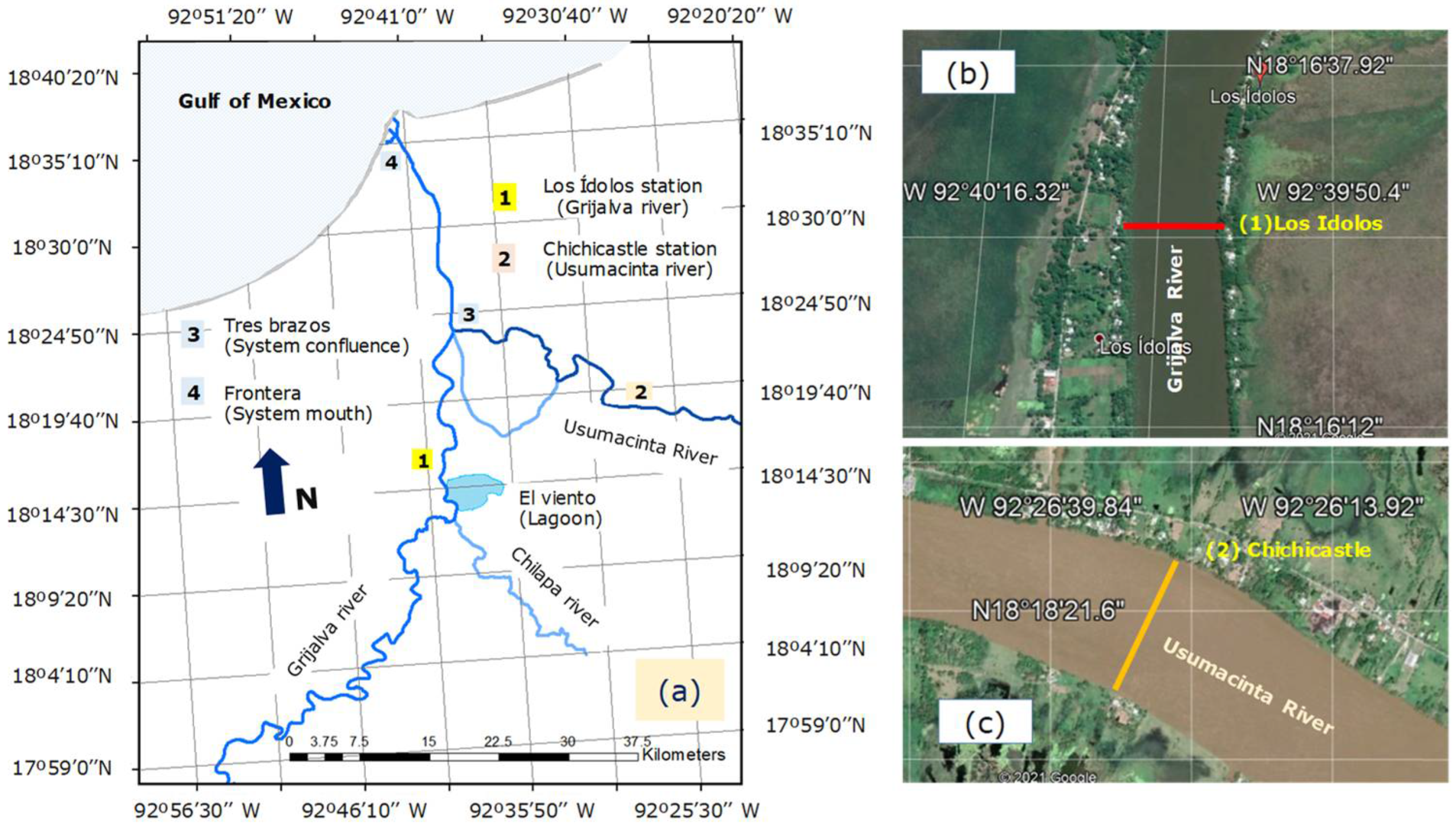
The sampling campaigns were conducted in the lower reaches of the Grijalva and Usumacinta rivers at Los Idolos over the Grijalva river and Chichicastle over the Usumacinta River; at coordinates 18°16.55′ N and 92°40.01′ E (Figure 1) and 18°18.48′ N and 92°26.67′ E (Figure 1). These sites are located 15 and 24 km before the confluence of both rivers, thus this study addressed the individual contributions of the Grijalva and Usumacinta main channels just before inflow to the Gulf of Mexico (Figure 1). The results are based on two sampling campaigns (each one took 3 days). One for the Usumacinta river in December 2016 and one for the Grijalva river in January 2017.
Concentration profiles were measured at 3 (Grijalva) and 4 (Usumacinta) columns distributed in the cross-section of the river (Figure 1b,c). At each column, between 5 and 8 (Grijalva) and 4 to 5 (Usumacinta) point samples at different depths were collected (by duplicate) using a Van Dorn bottle (volume: 2.2 L). A steel weight (2.5 kg) was attached to the sampler to improve alignment with the river streamlines. In addition, a composite water sample CWS (55 L in volume) was collected at the main channel area of each river, using samples from different depths (0.15 to 0.80 h, where h = local river depth). The point samples were used to determine the total suspended solids or simply local concentration (S) by gravimetric method, using fiberglass filters (4.7 cm in diameter, and 1.2 mm in particles retention limit), whereas CWS was used to investigate flocculation processes from experiments where PTV (particle tracking velocimetry) technique was applied (see next section). The Grijalva was sampled two times (D01 and N08), while the Usumacinta was sampled one time (D01) (N08: 10 October 2016 and D01: 12 January 2017).
Hydrodynamic parameters and turbulence properties in both rivers were obtained from ADCP (Acoustic Doppler Current Profiler, River Pro Teledyne instruments, Poway, CA, USA) data (velocities) recorded simultaneously during the sampling campaigns. In addition, we related the backscatter signals (BS) to the field concentrations (S) to calculate the instantaneous concentrations (s) from the instantaneous BS (by empirical fit). This allowed us to analyze data from three months of the 2016 high flow season: O10 (10 October 2016), N08, and D01. For each measurement, at least four transects were conducted across the river, using a boat to which the ADCP was attached. The ADCP used was a River Pro-Teledyne RD Instruments USA, operated in bottom track mode with a frequency and vertical resolution of 1200 kHz and 0.50 m, respectively. Hydraulic parameters derived from ADCP records are listed in Table 1.
2.2. Laboratory Analysis
The composite water samples were analyzed in the IITCA hydraulics laboratory using the rotating annular flume (RAF, manufactured at IITCA, Toluca, Mexico). Experiments in the RAF using samples from the Grijalva and Usumacinta rivers were performed at shear rates similar to those encountered in the field. For the Usumacinta an average value of u* = 0.07 m/s and for the Grijalva river an average value of u* = 0.04 m/s. This was possible using different rotation velocities of the base of the channel and the rotating cover that touches the water surface (Figure 2). However, results are only applicable for the high flow season.
The Rotating Annular Flume (RAF) is made of Plexiglass and has a 1.5 m diameter and a flume cross section of 15 cm × 15 cm (Figure 2). The cohesive sediments were analyzed during 2 h long experiments and images were taken each 15 min. The Particle Tracking Velocimetry (PTV), using the algorithm developed by [7] was applied. This implies two procedures; the first one improves image quality through spatial filtering, and the second procedure is detecting particles in each pulse. A double pulsed Nd-Yag laser (New wave Research, Fremont, CA, USA) of 50 mW was used and recorded with Lumenera CCD cameras (Teledyne Lumenera Ottawa, Canada).
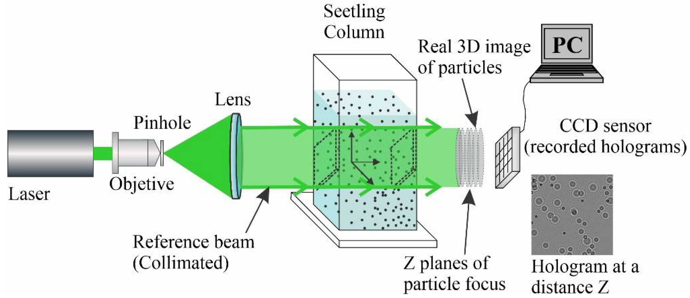
At the end of the experiments in the RAF, the aggregates are introduced in a settling column 1.0 m high and 3 cm × 7 cm cross-section, in order to obtain main flocs characteristics by means of an inline holographic system and DHPTV. In Figure 3, the main physical tools of an inline holographic system are shown. Comprising a Green light laser (B&W Tek Inc, Plainsboro Township, NJ, USA) of 532 nm of wave-length and 50 mW of power, an objective microscope 40×, a 10 μm pinhole in order to expand and filter the light shaft, a semispherical lens of 7 cm diameter and f = 75 mm, polarizing filters, digital camera CCD JAI CV-M2CL (JAI Ltd, Miyazaki, Japan) of 1600 × 1200 pixels spatial resolution and 7.4 µm per pixel and time resolution of 30 to 250 fps.
The inline holographic system sends a light shaft coherent and collimated, which goes through the fluid with the suspended particles and the light is dispersed forming the shaft named object which interferes with the original light shaft known as a reference in order to form a hologram that is captured by the CCD camera.
Once acquired and improved the holographic images were numerically reconstructed in order to obtain the 3D characteristics of the flocs. A computational algorithm was developed in MATLAB, using the convolution method [14]. To do so, it is required to know the parameters like camera pixels resolution, the pixel size in microns, and the wavelength of the laser. Using the reconstructed images, the PIV algorithm developed allowed us to determine flocs characteristics like size and position. Also, with the reconstructed images two algorithms for the box-counting method were also implemented, the classical BC according to [12] and the Triangular Box Counting method (TBC) [13] in order to obtain the fractal dimension of flocs.
The limitations of this holographic method are related to the number of particles analyzed per hologram, the method is focused on one particle and does not allow the presence of other particles. The size to be analyzed could go from 1 μm to 1.5 mm, not larger. To avoid measurement errors a calibration of the system and of the reconstruction methods was performed. In order to do so, polystyrene particles 50 μm in diameter were used, and the density parameters, lightning, and system collimation were adjusted. After applying reconstruction methods, the errors detected between 5 and 6.7% were considered acceptable.
2.3. Fractal Dimension Calculation by the Box Counting Method (BC-Method)
The fractal dimension (F) is obtained from the different gray levels of boxes in an image. Hence fractal dimension is calculated as the difference between the maximum gray level and the minimum according to the frame size of an image [12].
The following expression defines F
where represents the total number of boxes that cover an image and r is the box reduction factor.
This method counts the gray levels in the different frames of a holographic image. A level can be calculated using the reduced scale length of the image in relation to the maximum gray level, which can be represented by:
where is the gray level, L is the box length, G is the maximum level of gray intensity in an image and M is the image length. In order to obtain a reduction factor of 1/r, the length of the reduced scale can be obtained using the box length L related to the image length M. Thus
For an image of size M × M and assuming the box size L × L, thus all the image is covered by frames of size The fractal dimension F of an aggregate corresponds to the slope of a logarithmic graph of Nr vs. 1/r, where Nr is the number of frames with at least a gray level that covers the image for each r value.
2.4. Triangular Box Counting Method (TBC-Method)
This method improves the box-counting method and was proposed by Kaewaramsri and Woraratpanya [13]. The square boxes are divided into triangular boxes of the same size. The steps to follow are the following:
Divide M × M píxels images in square boxes of size, r from 2 to M/2.
Define box height h = r × G/M where G is the total number of gray levels. The box size is r × r × h.
The latter technique is applied to each box. Results are shown in Figure 4. There are two patterns, p1 and p2, p1 are the up and down right diagonals, and p2 are up and down left diagonals.
Obtain the box and each pattern so that l and k can be calculated by IMax/h and IMin/h, where IMax and IMin are the maximum and minimum values of intensity in each frame.
Obtain p1 averaging up and down right diagonals, and p2 averaging up and down left diagonals.
Obtain every nbox recount using
Use to calculate the total number of recount boxes Nr.
2.5. Models for Fractal Dimension Calculation
Two models were used to fit the data obtained by holography.
The first model was the fit proposed by García-Aragon et al. [15] and obtained experimentally with sediments coming from aquaculture tanks
where the constants a and n depend on the type of sediment, n represents the exponent of the Particle Reynolds number (Rep) when calculating the permeable drag coefficient (CDf) and a is a constant (CDf = a/Repn).
The second was obtained with the equation proposed by Lau and Krishnappan [16] for effective floc density in conjunction with the respective Kranenburg [2] equation, getting the following equation (see Garcia-Aragon et al. [16]):
where F is the fractal dimension, D is floc diameter, d is the primary particle diameter and constants b and c are empirical coefficients that depend on the type of sediment.
3. Results
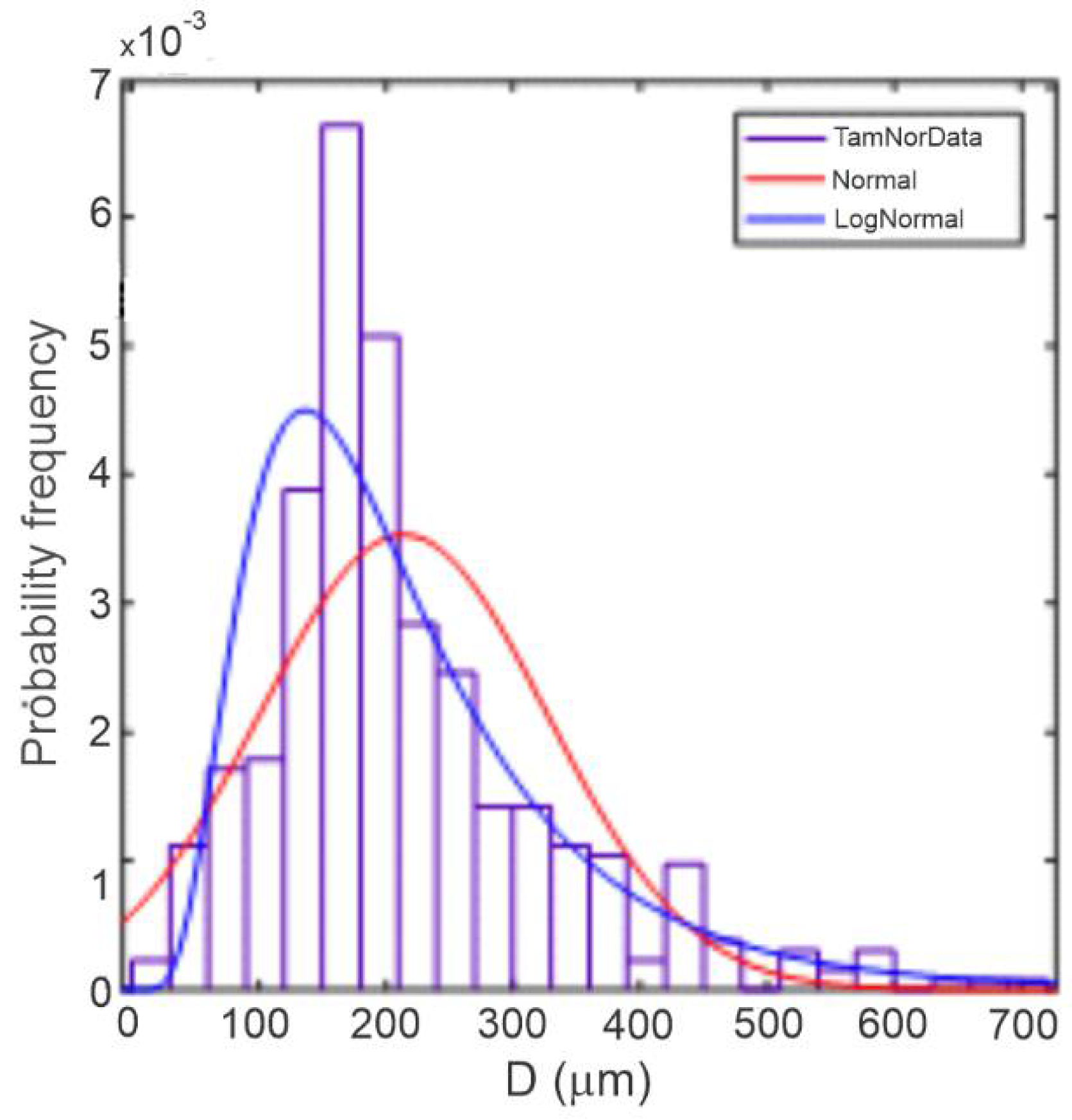
From the RAF experiments, the size of aggregates was obtained at different flocculation times. Then samples of particles for each flocculation time were selected and analyzed in a glass settling column with DHPTV. The average floc size was found to increase with time. For the Usumacinta river, the frequency of sizes is shown in Figure 5, after a flocculation time, t = 45 min.
For this elapsed time, the sample consisted of 657 particles with diameters ranging from 39.2 to 514.1 μm, with an average value of 197.4 μm using a lognormal fit.
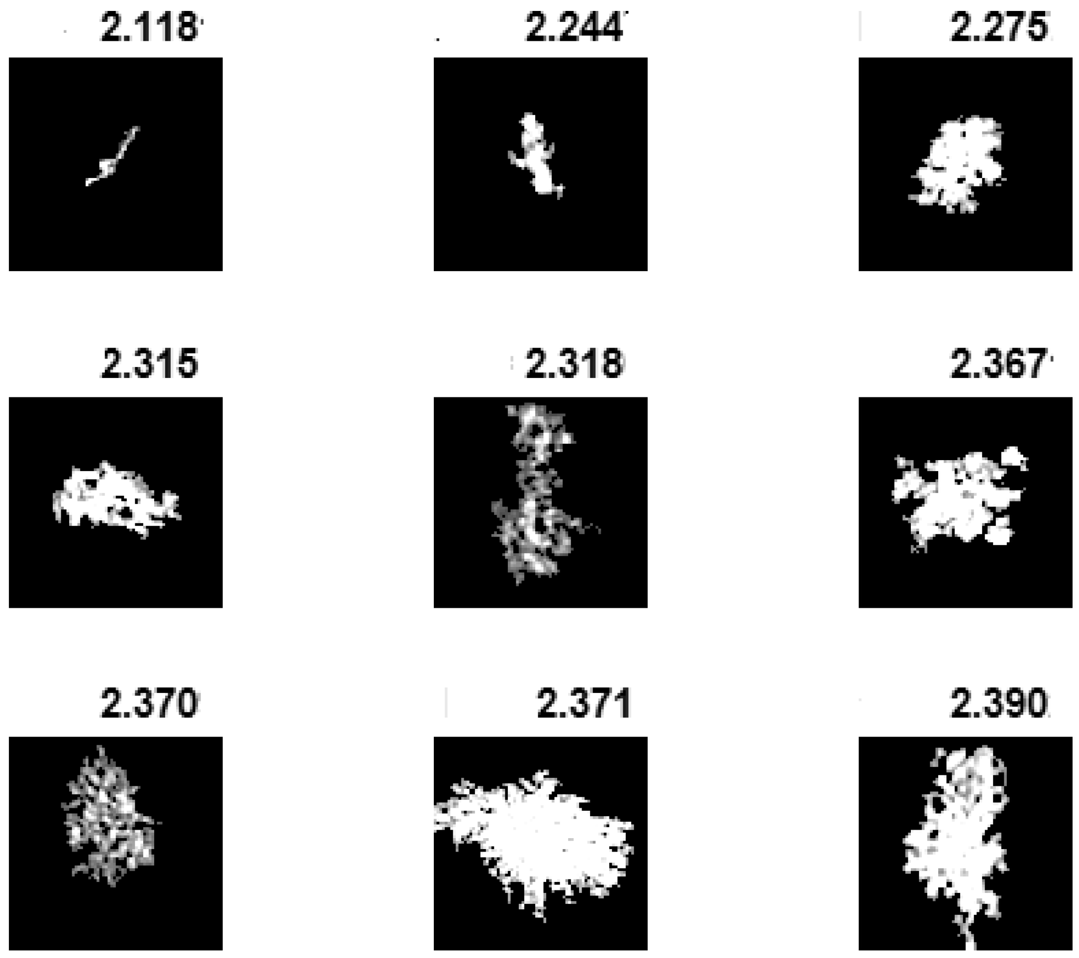
Figure 6 shows fractal dimensions calculated from hologram reconstruction for the Usumacinta River sediment for the flocculation time of 45 min.
Figure 7 shows that the floc diameters in the Grijalva river are larger (average value of 285 μm) than those of the Usumacinta (average value of 197 μm).
Figure 8 shows that during the first 45 min the floc diameter increases sharply then diminishes slowly and finally reaches an almost stable value.
The fractal dimension against the floc diameter was plotted and adjusted for each river (Usumacinta and Grijalva) at different flocculation times, with the models proposed in this research (Equations (5) and (6)).
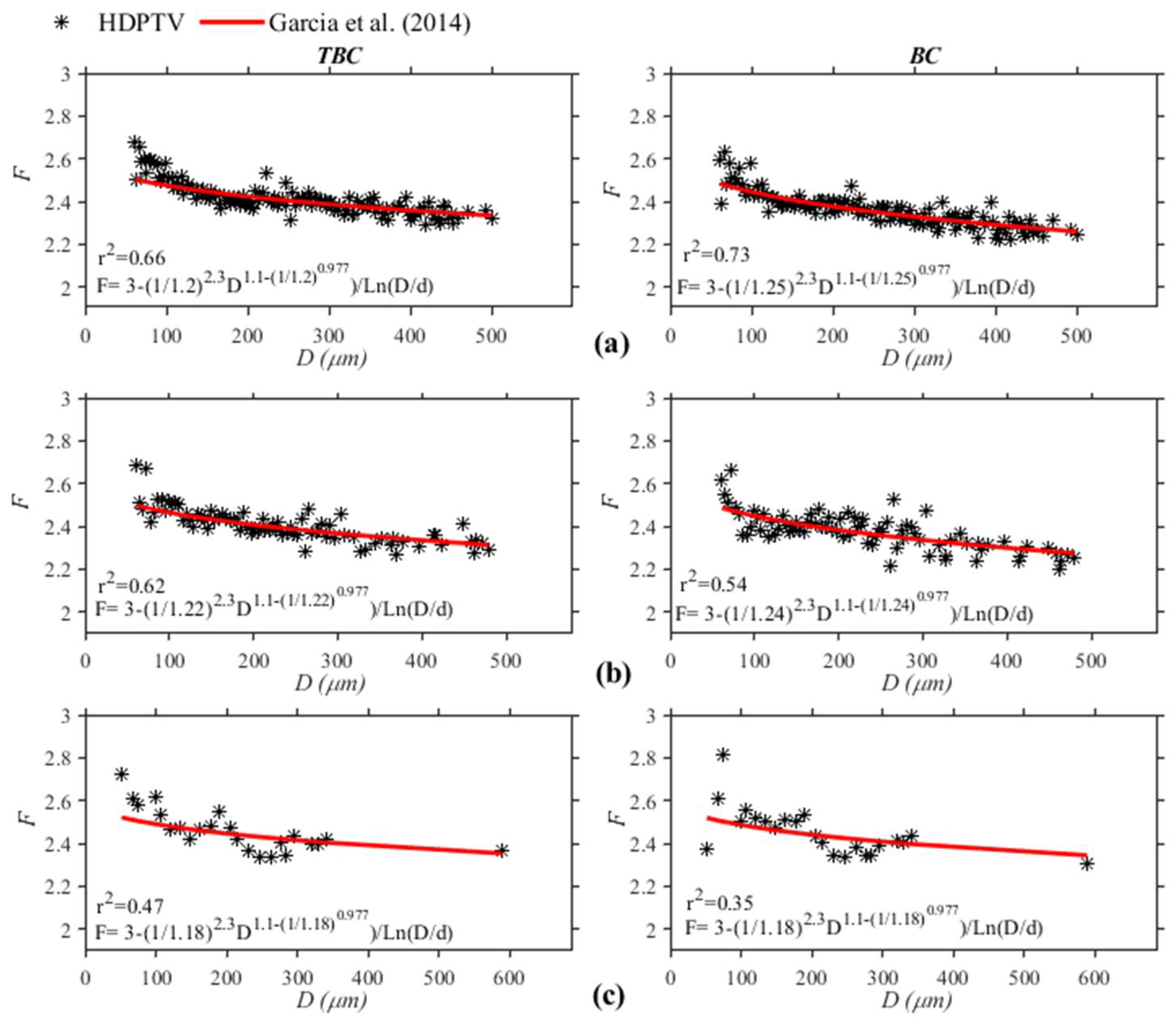
Figure 9 shows the best fit obtained with the model Equation (5). The value of the parameters obtained were; a value of n = 1.15 and a value of “a” varying between 1.18 and 1.22 for the different flocculation times analyzed. The triangular box-counting method (TBC) presented better determination coefficients than the classical box-counting method. The size of the primary particle diameter used for the Usumacinta River was 5 μm, which will be discussed later.
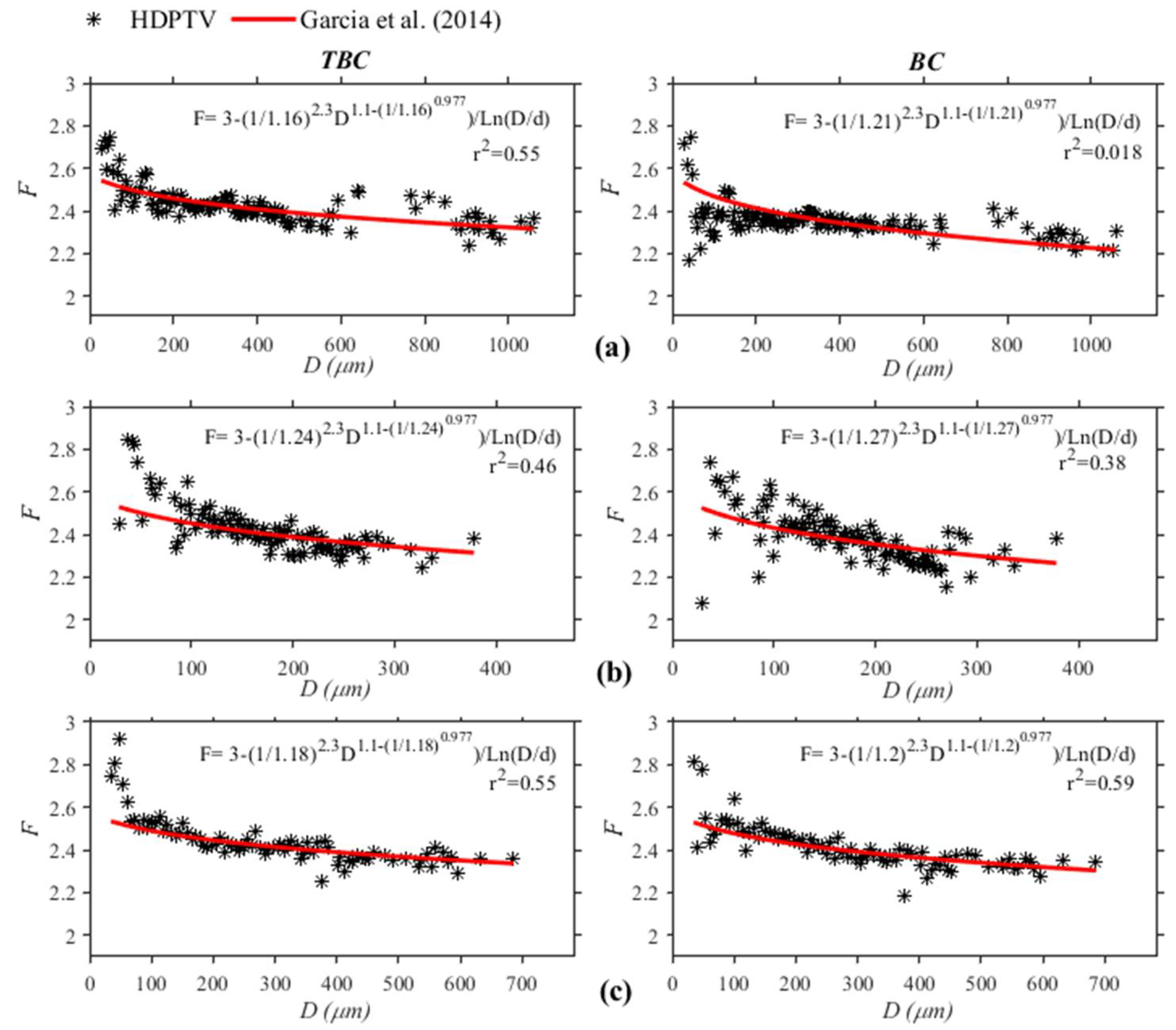
Figure 10 shows the best fit obtained with Equation (5). The value of the parameters obtained were a value of n = 1.15 and a value of “a” varying between 1.16 and 1.24 for the different flocculation times analyzed. The triangular box-counting method presents better determination coefficients than the classical box-counting method. The size of the primary particle diameter used for the Grijalva river was 10 μm, which will be discussed later. It is observed comparing Figure 7 and Figure 8, that for small aggregates diameter the F in the Grijalva tends to be larger than the corresponding one in the Usumacinta. This is not true for larger diameters, indicating larger flocculation in the Grijalva than in the Usumacinta. This can be related to the larger turbulence in the Usumacinta River, able to produce more breakage of aggregates.
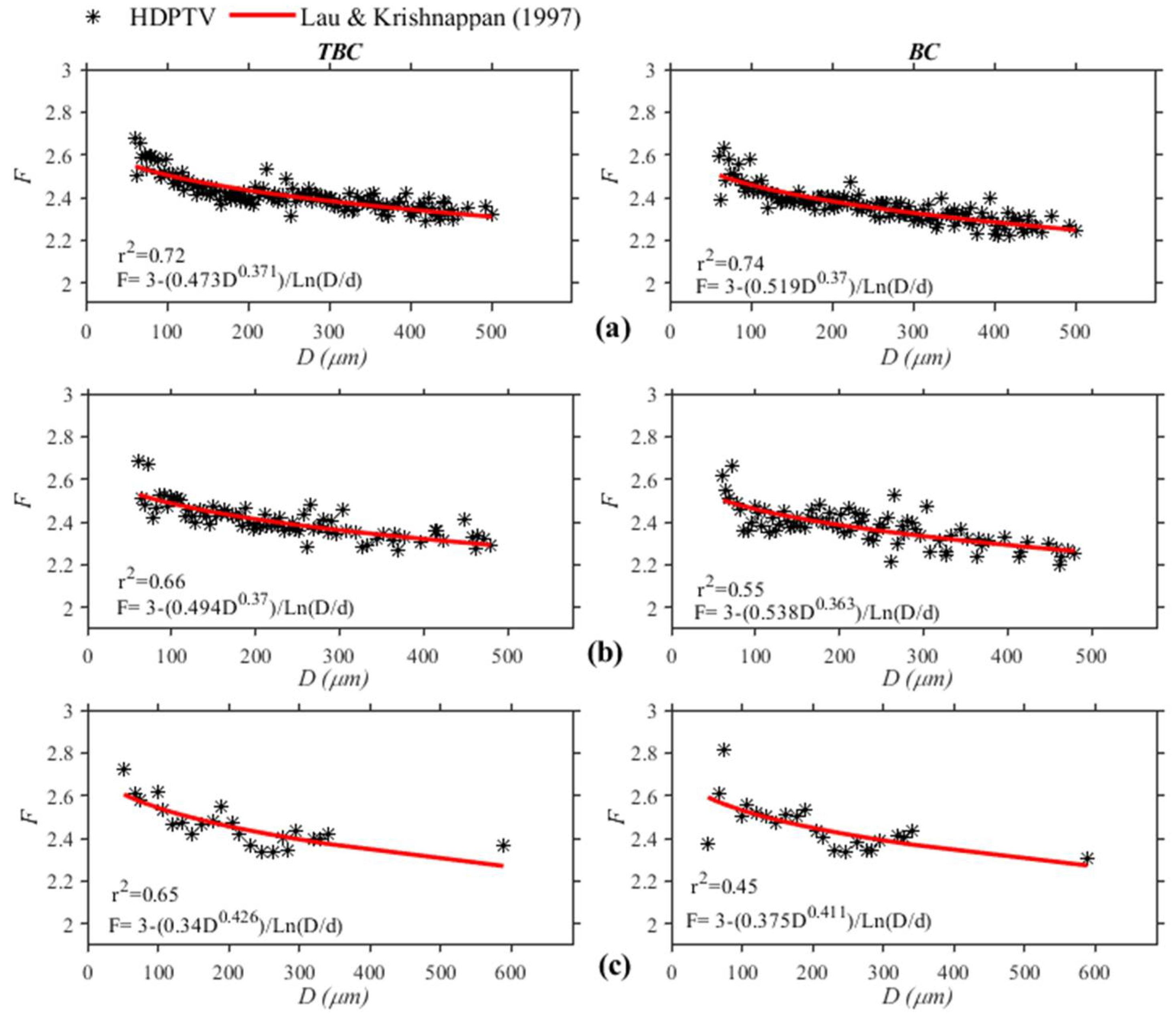
Figure 11 shows the best fit obtained with Equation (6), with b varying between 0.34 and 0.494 in the TBC method and c between 0.37 and 0.426. for the different flocculation times analyzed. The triangular box-counting method presents better determination coefficients than the classical box-counting method. The size of the primary particle diameter used for the Usumacinta River was 5 μm, which will be discussed later.
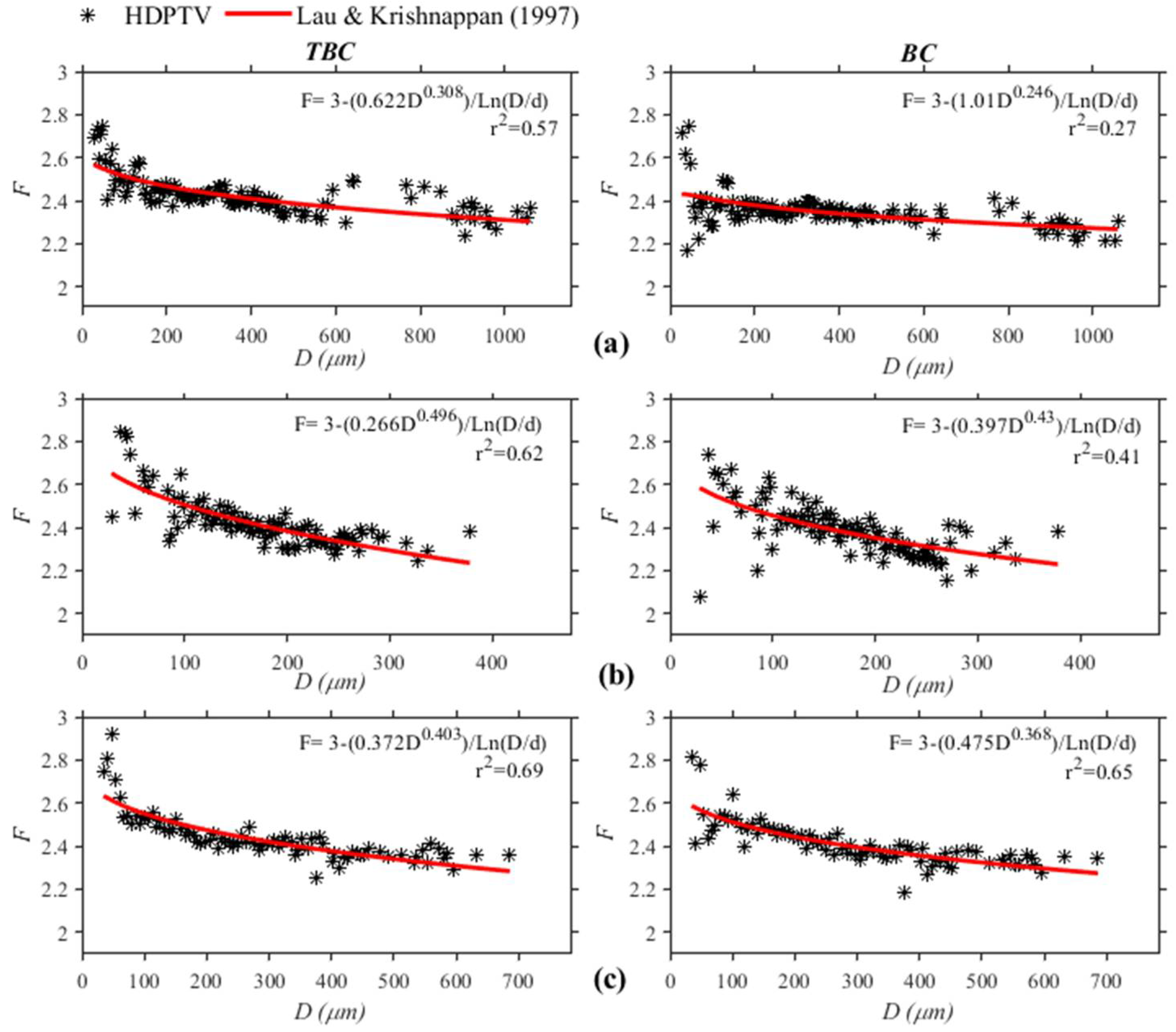
Figure 12 shows the best fit obtained with Equation (6), with b varying between 0.266 and 0.622 in the TBC method, and c between 0.308 and 0.496. for the different flocculation times analyzed. The triangular box-counting method presents better determination coefficients than the classical box-counting method. The size of the primary particle diameter used for the Grijalva river was 10 μm, which will be discussed later.
4. Discussion
The fractal dimension data for rivers are rather limited as much of the research in this area was carried out in the ocean and estuaries, using specialized in-situ optical instruments. The average size in the Grijalva river flocs is similar to the one found in the PO river delta which is 370 μm [17]. In this delta, large flocculation was shown to exist, and the shear velocity is low due to calmer hydrodynamic conditions. There is no data relating to the fractal dimension of PO river delta flocs, but they state that for a 200 μm floc size the average effective density is 100 kg/m3, which is similar to the one found in this study. Van der Lee [18] measured in situ floc size and settling velocity in the Dollard estuary, Holland using underwater video cameras-UVC. He found flocs size varying from 100 to 300 μm with densities varying from 1500 to 1100 kg/m3 for a concentration of 350 mg/L. Using Kranenburg [2] equation, one can show that the floc densities of Grijava River sediment and the Usumacinta River sediments are in the range of floc densities found in the Dollard estuary. Xia et al. [19] measured floc sizes and settling velocities in the Pearl River estuary, China using LISST and found very small flocs (size under 96 μm).
With respect to the primary particle diameter to be used in these models, a useful relationship has been presented by Maggi [20] after comparing flocs of different composition mineral, biomineral, and biological particles. He found that the primary particle diameter d is related to the floc density as d = −(2.76 × 10⁻⁹)ρf + 7.32 × 10⁻⁶. This relationship gives the primary particle diameter for the Usumacinta River as 4.2 μm and for the Grijalva river as 4.1 μm. The former is very similar to the one used in this research for the Usumacinta River and the latter is almost half the one used for the Grijalva river. Many et al. [21] measured floc size and settling velocity in the Rhone estuary using LISST and found that primary particle diameters varied from 1 to 12 μm. Their analysis was able to show that the fractal dimension varied from 2.0 to 2.5, which agrees with the values found in this research.
The models proposed in this research to calculate the fractal dimension have parameters that need some experimental work to be properly defined. For Equation (5) the parameter n could be maintained constant n = 1.15 in the data analyzed, it has been shown that this parameter has a small range of variation for different types of sediments from 1.1 to 1.25 [16]. The parameter “a” has shown variation from 1.16 to 1.24 and it depends on the type of sediment. An average value of 1.2 could be used with confidence for the Usumacinta River and 1.22 for the Grijalva river.
Concerning Equation (6), the parameters b and c measured for a number of rivers in Canada and the United Kingdom were summarized by Krishnappan [22]. The values corresponding to the Steepbank River in Alberta, Canada (b = 0.61 and c = 0.35) are within the range of values obtained in the present study (b varied from 0.266 to 0.622 and c varied from 0.308 to 0.496). Knowing the values of b and c, the settling velocity of the flocculated sediment can be calculated using a modified Stokes’ equation as given in Krishnappan [22]:
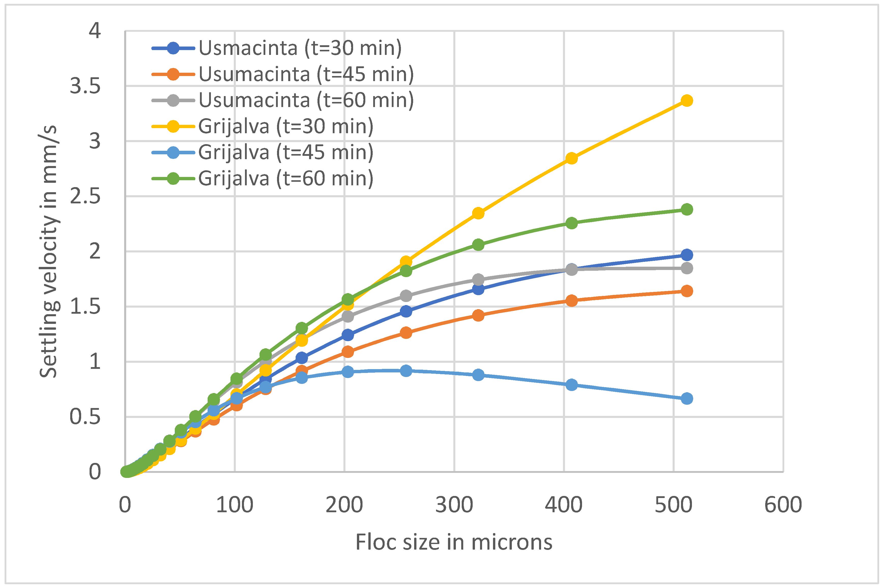
where is the settling velocity of the kth fraction of sediment and ν is the kinematic viscosity of water and g is the acceleration due to gravity. Applying Equation (7) to the flocs at various elapsed times, the settling velocity of sediments flocs from Usumacinta and Grijalva Rivers were calculated as shown in Figure 13.
From Figure 11, one can see that there is a greater variability of settling velocity for the Grijalva River sediment in comparison to the Usumacinta River sediment as these sediments were undergoing flocculation. For the Grijalva River sediment, the maximum set tling velocity varies from 0.67 to 3.4 mm/s, whereas for the Usumacinta River sediment the maximum velocity variations are comparatively smaller in the range of 1.97 to 1.64 mm/s. From the settling velocity distributions given in Figure 11, one can see that the Usumacinta River sediment behaves differently from the Grijalva River sediment during floc reconstruction because of the different hydrodynamic conditions and the properties of sediment-water mixtures between these two rivers. The differences in the settling velocities are also reflected in the fractal dimensions of the sediment flocs.
Recent research highlights the importance of organic matter on freshwater floc formation [23], until appropriate models will be developed to include this variable, suspended sediment samples and empirical models like the ones presented in this paper remain useful.
5. Conclusions
It can be concluded from the present study that floc characteristics can be analyzed in laboratory experiments after floc reconstruction by means of a Rotating Annular Flume (RAF). This can be an alternative approach to costly equipment involved in in-situ sampling of flocs that are often carried out in ocean research. In addition, the Digital Holography for Particle Tracking Velocimetry (DHPTV) is an efficient tool to obtain flocs fractal dimension. The present study has also shown that the models of Garcia-Aragon [15] and Lau and Krishnappan [16] can reliably predict the Fractal dimension of the flocculating sediment once the sizes of the sediment flocs are known in freshwater environments. It is known that optical equipment working with laser technology does not perform well in environments with high velocity like in rivers. Until such limitation is overcome, the use of laboratory tools able to reproduce the hydrodynamic of river environments could be safely used.
Author Contributions
H.Z.M. helped with methodology, validation, formal analysis, and investigation. J.A.G.A. helped with conceptualization, formal analysis, and writing-original draft preparation. H.S.T. helped with methodology, software elaboration, and formal analysis. B.G.K. helped with methodology, investigation, and writing-review. All authors have read and agreed to the published version of the manuscript.
Funding
The first author received a scholarship from CONACYT the Mexican government research funding agency Macsag1117.
Informed Consent Statement
Not applicable.
Data Availability Statement
Not applicable.
Conflicts of Interest
The authors declare no conflict of interest.
References
- Droppo, I.G. Rethinking what constitutes suspended sediment. Hydrol. Process. 2001, 14, 653–667. [Google Scholar] [CrossRef]
- Kranenburg, C. The fractal structure of cohesive sediment aggregates. Estuar. Coast. Shelf Sci. 1994, 39, 1665–1680. [Google Scholar] [CrossRef]
- Bouchez, J.; Metivier, F.; Lupker, M.; Maurice, L.; Perez, M.; Gaillardet, J.; France-Lanord, C. Prediction of depth-integrated fluxes of suspended sediment in the Amazon River: Particle aggregation as a complicating factor. Hydrol. Process. 2011, 25, 778–794. [Google Scholar] [CrossRef]
- Jordan, P.R. Fluvial Sediment of the Mississippi River at St. Louis, Missouri; USGS Water-Supply Paper 1802; United States Government Printing Office: Washington, DC, USA, 1965.
- Scott, C.H.; Stephens, H.D. Special Sediment Investigations: Mississippi River at St. Louis, Missouri; Water Supply Paper 1819; United States Government Printing Office: Washington, DC, USA, 1966. [CrossRef]
- Li, W.; Wang, J.; Yang, S.; Zhang, P. Determining the existence of the fine sediment flocculation in the Three Gorges Reservoir. J. Hydraul. Eng. 2015, 141, 5014008. [Google Scholar] [CrossRef]
- Salinas-Tapia, H.; Garcia-Aragon, J.A.G.; Hernandez, D.M.; Garcia, B.B. Particle Tracking Velocimetry (PTV) Algorithm for Non-uniform and Nonspherical Particles. In Proceedings of the Electronics, Robotics and Automotive Mechanics Conference (CERMA’06), Cuernavaca, México, 26–29 September 2006; Volume II. [Google Scholar]
- Salinas, T.H.; Robles, R.C.O.; Chávez, C.D.; Bautista, C.C.F. Caracterización geométrica y cinemática de un chorro pulverizado empleando la técnica óptica PTV. Tecnologia y Ciencias del Agua 2014, 5, 125–140. [Google Scholar]
- Félix-Félix, J.R.; Salinas-Tapia, H.; Bautista, C.; García-Aragón, J.; Burguete, J.; Playán, E. A modified particle tracking velocimetry technique to characterize sprinkler irrigation drops. Irrig. Sci. 2017, 35, 515–531. [Google Scholar] [CrossRef]
- López, R.B.; Salinas, T.H.; García, P.D.; Durán, G.D.; Gallego, A.I.; Fonseca, O.C.; Garcia, A.J.A.; Díaz, D.C. Performance study of annular settler with gratings in circular aquaculture tank using computational fluid dynamics. Aquac. Eng. 2021, 92, 102143. [Google Scholar] [CrossRef]
- Malek, M.; Allano, D.; Coëtmellec, S.; Lebrun, D.; Özkul, C. Digital in-line holography for three-dimensional-two-components particle tracking velocimetry. Meas. Sci. Technol. 2004, 15, 699–705. [Google Scholar] [CrossRef]
- Long, M.; Peng, F. A Box-counting Method with adaptable box height for measuring the fractal feature of images. Radio Eng. 2013, 22, 208–2013. [Google Scholar]
- Kaewaramsri, Y.; Woraratpanya, K. Improved Triangle Box-Counting Method for Fractal Dimension Estimation. In Recent Advances in Information and Communication Technology; Unger, H., Meesad, P., Boonkrong, S., Eds.; Advances in Intelligent Systems and Computing; Springer: Cham, Switzerland, 2015; Volume 361. [Google Scholar] [CrossRef]
- Coronel, A.W. Optomecatronics, Sistema Para Medir Velocidad en Flujo de Fluidos en 3D. Master’s Thesis, Centro de Investigaciones en Óptica, León, Guanajuato, México, 2011. [Google Scholar]
- Garcia-Aragon, J.A.; Salinas-Tapia, H.; Moreno-Vega, J.; Diaz-Palomarez, V.; Tejeda-Vega, S. A model for the settling velocity of flocs; Application to an aquaculture recirculation tank. Int. J. Comput. Methods Exp. Meas. 2014, 2, 313–322. [Google Scholar] [CrossRef] [Green Version]
- Lau, Y.L.; Krishnappan, B.G. Measurement of size distribution of settling flocs. In NWRI Publication No. 97-223; National Water Research Institute, Environment Canada: Burlington, ON, Canada, 1997. [Google Scholar]
- Fox, J.M.; Hill, P.S.; Milligan, T.G.; Boldrin, A. Flocculation and sedimentation n the Po River Delta. Mar. Geol. 2004, 203, 95–107. [Google Scholar] [CrossRef]
- Van der Lee, W.T.B. Temporal variation of floc size and settling velocity in the Dollard estuary. Cont. Shelf Res. 2000, 20, 1495–1511. [Google Scholar] [CrossRef]
- Xia, X.M.; Li, Y.; Yang, H.; Wu, C.Y.; Sing, T.H.; Pong, H.K. Observations on the size and settling velocity distributions of suspended sediment in the Pearl River Estuary, China. Cont. Shelf Res. 2004, 24, 1809–1826. [Google Scholar] [CrossRef]
- Maggi, F. The settling velocity of mineral, biomineral and biological particles and aggregates in water. J. Geophys. Res. 2013, 118, 22118–22132. [Google Scholar] [CrossRef]
- Many, G.; de Madron, X.D.; Verney, R.; Bourrin, F.; Renosh, P.R.; Jourdin, F.; Gangloff, A. Geometry, fractal dimension and settling velocity of flocs during flooding conditions in the Rhône ROFI. Estuar. Coast. Shelf Sci. 2019, 219, 1–13. [Google Scholar] [CrossRef]
- Krishnappan, B.G. Review of a semi-empirical modelling approach for cohesive sediment transport in river systems. Water 2022, 14, 256. [Google Scholar] [CrossRef]
- Walch, H.; von der Kammer, F.; Hofmann, T. Freshwater Suspended Particulate Matter–Key Components and Processes in Floc Formation and Dynamics. Water Res. 2022, 220, 118655. [Google Scholar] [CrossRef] [PubMed]
Figure 1.
Location of Chichicastle #2 (Usumacinta) and Los Idolos # 1 (Grijalva) sampling stations. (a) Overall location, (b) los idolos cross section, (c) Chichicastle cross section.
Figure 1.
Location of Chichicastle #2 (Usumacinta) and Los Idolos # 1 (Grijalva) sampling stations. (a) Overall location, (b) los idolos cross section, (c) Chichicastle cross section.

Figure 2.
Experimental setup for tests in Rotating Annular Flume (RAF).

Figure 3.
In-line Digital Holography set up.

Figure 4.
Division of frame image in two triangular frames with four patterns (a) up triangular (b) down triangular (c) left triangular (d) right triangular.
Figure 4.
Division of frame image in two triangular frames with four patterns (a) up triangular (b) down triangular (c) left triangular (d) right triangular.

Figure 5.
Frequency of diameters for the Usumacinta at t = 45 min after RAF experiments.

Figure 6.
Flocs fractal dimension obtained after 45 min in RAF for the Usumacinta River sediment.

Figure 7.
Frequency of diameters for the Grijalva at t = 60 min after RAF experiments.

Figure 8.
Time evolution of floc diameter in RAF experiments for the Grijalva river. Circles are experimental values and doted line the trend with time.
Figure 8.
Time evolution of floc diameter in RAF experiments for the Grijalva river. Circles are experimental values and doted line the trend with time.

Figure 9.
Best fit of the fractal dimension for the Usumacinta River with Garcia Aragon et al. [16] model at different flocculation times using TBC and BC methods; (a) 30 min, (b) 45 min, (c) 60 min.
Figure 9.
Best fit of the fractal dimension for the Usumacinta River with Garcia Aragon et al. [16] model at different flocculation times using TBC and BC methods; (a) 30 min, (b) 45 min, (c) 60 min.

Figure 10.
Best fit of the fractal dimension for the Grijalva River with Garcia Aragon et al. [16] model at different flocculation times using TBC and BC methods; (a) 30 min, (b) 45 min, (c) 60 min.
Figure 10.
Best fit of the fractal dimension for the Grijalva River with Garcia Aragon et al. [16] model at different flocculation times using TBC and BC methods; (a) 30 min, (b) 45 min, (c) 60 min.

Figure 11.
Best fit of the fractal dimension for the Usumacinta River with Lau and Krishnappan [15] model at different flocculation times using TBC and BC methods; (a) 30 min, (b) 45 min, (c) 60 min.
Figure 11.
Best fit of the fractal dimension for the Usumacinta River with Lau and Krishnappan [15] model at different flocculation times using TBC and BC methods; (a) 30 min, (b) 45 min, (c) 60 min.

Figure 12.
Best fit of the fractal dimension for the Grijalva River with Lau and Krishnappan [15] model at different flocculation times using TBC and BC methods; (a) 30 min, (b) 45 min, (c) 60 min.
Figure 12.
Best fit of the fractal dimension for the Grijalva River with Lau and Krishnappan [15] model at different flocculation times using TBC and BC methods; (a) 30 min, (b) 45 min, (c) 60 min.

Figure 13.
Settling velocity distributions for Usumacinta and Grijalva River sediments.


Table 1.
Main hydraulic parameters obtained with ADCP for the period October–December 2016.
| Hydraulic Parameters | Grijalva | Usumacinta |
|---|---|---|
| Flow rate (m3/s) | 1420–1055 | 2085–1755 |
| Top width (m) | 200–185 | No data |
| Mean velocity (m/s) | 0.71–0.54 | 0.79–0.7 |
| Maximum depth (m) | 13.2–12.2 | 9.9–9.1 |
Publisher’s Note: MDPI stays neutral with regard to jurisdictional claims in published maps and institutional affiliations. |
© 2022 by the authors. Licensee MDPI, Basel, Switzerland. This article is an open access article distributed under the terms and conditions of the Creative Commons Attribution (CC BY) license (https://creativecommons.org/licenses/by/4.0/).
Share and Cite
MDPI and ACS Style
Zepeda Mondragon, H.; Garcia Aragon, J.A.; Salinas Tapia, H.; Krishnappan, B.G. Estimation of Fractal Dimension of Suspended Sediments from Two Mexican Rivers. Water 2022, 14, 2774. https://doi.org/10.3390/w14182774
AMA Style
Zepeda Mondragon H, Garcia Aragon JA, Salinas Tapia H, Krishnappan BG. Estimation of Fractal Dimension of Suspended Sediments from Two Mexican Rivers. Water. 2022; 14(18):2774. https://doi.org/10.3390/w14182774
Chicago/Turabian StyleZepeda Mondragon, Hilda, Juan Antonio Garcia Aragon, Humberto Salinas Tapia, and Bommanna G. Krishnappan. 2022. "Estimation of Fractal Dimension of Suspended Sediments from Two Mexican Rivers" Water 14, no. 18: 2774. https://doi.org/10.3390/w14182774
Note that from the first issue of 2016, this journal uses article numbers instead of page numbers. See further details here.