Mathematical Model for the Movement of Two-Pipe Vehicles in a Straight Pipe Section

Abstract

In the design process for a two-pipe vehicles transportation system, some simple mathematical models are required to quickly calculate the main characteristics of the system. For this purpose, an easy-to-handle mathematical model for the concentric annular gap flow is proposed, and the velocity expression for the concentric annular gap flow is solved using cylindrical coordinates. According to the force characteristics of the two-pipe vehicles, a mathematical model of the two-pipe vehicle motion is established, and the motion and force balance equations of the two-pipe vehicles are deduced. The experimental results are in good agreement with the model results. The factors affecting the two-pipe vehicles movement speed are analyzed, and the standard regression coefficient method in multiple regression analysis is used to determine the influence degree of each factor on the movement speed of the two-pipe vehicles. The research presented in this paper not only enriches the annular gap flow theory, but also provides a theoretical reference for the development of the two-pipe vehicles transportation technology and provides technical support for the realization of relevant industrial applications.

1. Introduction

With the rapid development of the social economy and technology, the speed of material exchange between regions is constantly increasing, and the weight of material transportation is also increasing. Such continuous development of material exchange also creates new requirements for material conveying methods [1,2]; however, due to the problems related to high resource consumption, high transportation cost, and high consumption of human resources, traditional material transportation methods can no longer meet the currently advocated green, environmentally friendly, and efficient development concepts [3,4]. Therefore, there is an urgent need for new transportation methods to address the above problems. Along these lines, a new technology of hydraulic transportation using a capsule pipeline has been proposed. This technology mainly stores the materials in a closed container, avoiding contact between the materials and the transportation medium, and can directly transport various materials, such as gases, liquids, and solids [5,6]. Therefore, it is of great practical significance to study capsule pipeline hydraulic transportation technology [7].

In 1960, the Alberta Research Center in Canada first proposed the concept of capsule pipeline hydraulic transportation technology [8]. In the early stages, the model test and theoretical analysis was mainly used to study the velocity of the capsule and the change of the pressure in the pipeline [9,10,11,12]. With the rapid development of computer technology, more and more scholars have used numerical simulation methods to study capsule pipeline hydraulic transportation technology. The research in this period also mainly focused on the force characteristics, flow field distribution, and vorticity change regarding the capsule during movement [13,14,15,16]. In 1991, the Capsule Pipeline Research Center was established at the University of Missouri, Columbia, and the center has gradually commercialized capsule pipeline hydraulic transportation technology. As this technology is more commonly used in commercial production, many scholars have extended their research direction to drag reduction and delivery system optimization during capsule movement [17,18,19,20,21]. The existing research on this technology has achieved many results; however, the defects and deficiencies of this transportation technology have been gradually exposed. For example, the capsule cannot be kept in a suspended state at all times during movement, and collision and friction will occur between the capsule and the wall of the pipeline, greatly reducing the service life of the pipeline and increasing the energy consumption. Furthermore, it is not conducive to the transportation of fragile materials [22]. Therefore, in order to address the above problems, the tube-contained raw materials pipeline hydraulic transportation technology has been proposed [23].

The tube-contained raw materials pipeline hydraulic transportation technology mainly involves adding supports to both ends of the capsule, such that the capsule is always in a concentric state with the pipeline during the movement process, which avoids collisions between the capsule and the pipeline [24]. Current research on this technology mainly focuses on the motion and hydraulic characteristics of a single pipe vehicle [25,26,27,28,29]; however, with the continuous increase in transportation volumes, the load capacity of a single pipe vehicle can no longer meet the current development requirements and, therefore, it is necessary to study the transportation of pipeline trains [30,31].

As the smallest conveying unit in the pipeline train, two-pipe vehicles have been relatively less researched to date [32,33]. In two-pipe vehicles transportation systems, the transportation speed of the two-pipe vehicles is an important reference index in the design of the system. It not only determines the energy loss of the technology during the transportation process, but also directly affects the transportation efficiency. Therefore, it is necessary to study the transportation speed of two-pipe vehicles [34,35]. However, the commonly used model experiments can only study the moving speed of a limited number of types of pipe vehicle, and the obtained test results have certain limitations regarding the application of this technology. Therefore, establishing a reasonable mathematical model of two-pipe vehicles remains a key problem in popularizing the technology.

In this paper, according to concentric annular gap flow theory and the force characteristics of two-pipe vehicles, a mathematical model for the stable movement of the two-pipe vehicles in a straight pipeline is constructed, and the accuracy of the mathematical model is verified through a model experiment. The mathematical model includes various influencing factors that affect the movement speed of the two-pipe vehicles, providing a theoretical basis for subsequent analysis of the relationship between each factor and the two-pipe vehicles movement speed. This mathematical model can quickly determine the transportation speed of the two-pipe vehicles, providing technical guidance for the construction of two-pipe vehicles transportation systems, as well as a theoretical basis for obtaining the optimal transportation speed of two-pipe vehicles.

2. Establishment of Mathematical Models

2.1. Mathematical Model of Concentric Annular Gap Flow

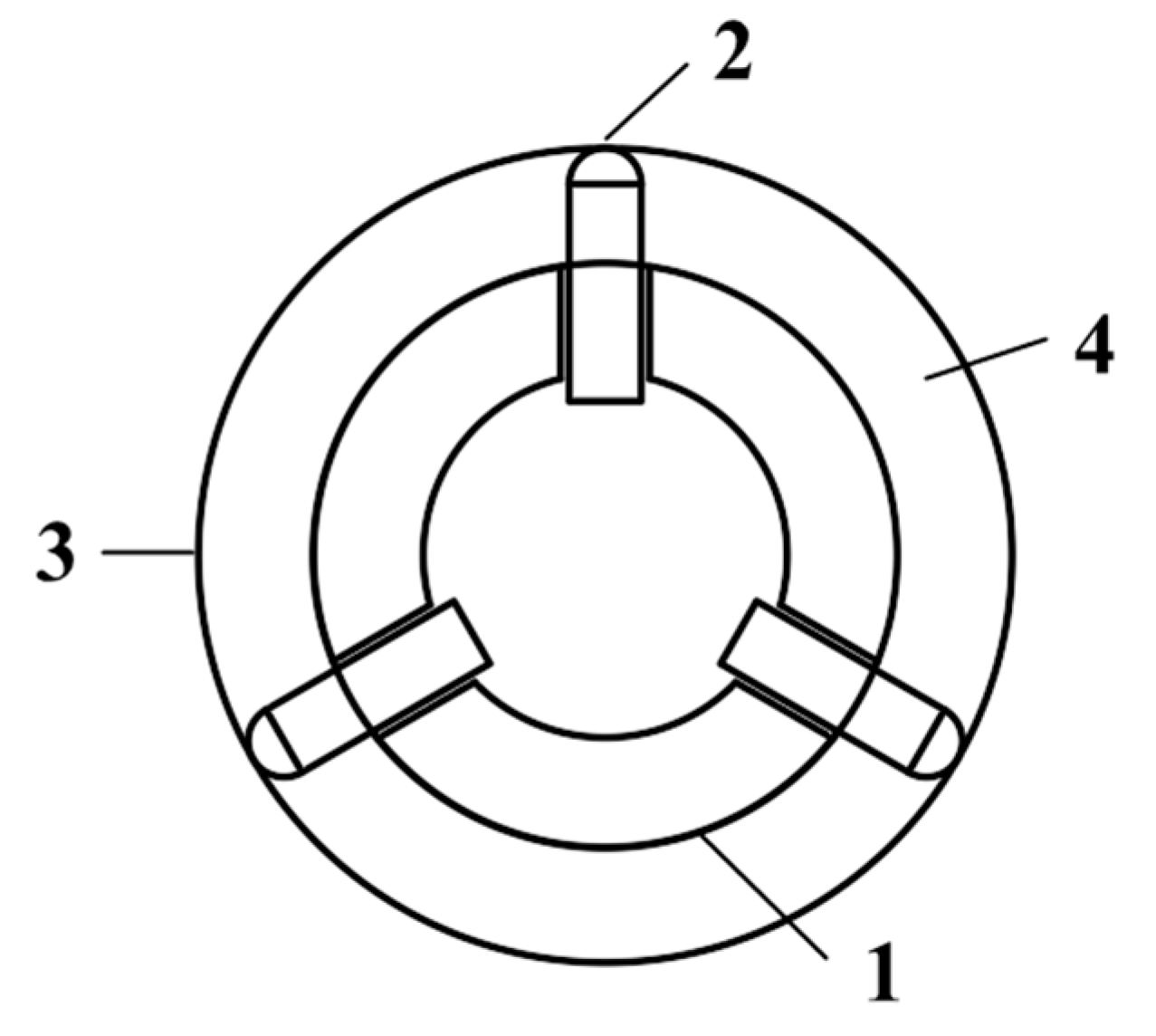
As the two-pipe vehicles and the pipeline are in a concentric state, a concentric annular gap is formed between the wall surface of the two-pipe vehicles and the pipe wall, as shown in Figure 1. The water flow in the concentric annular gap not only affects the movement speed of the two-pipe vehicles, but also affects the energy loss. Therefore, it is necessary to understand the flow velocity variation in the concentric annular gap.

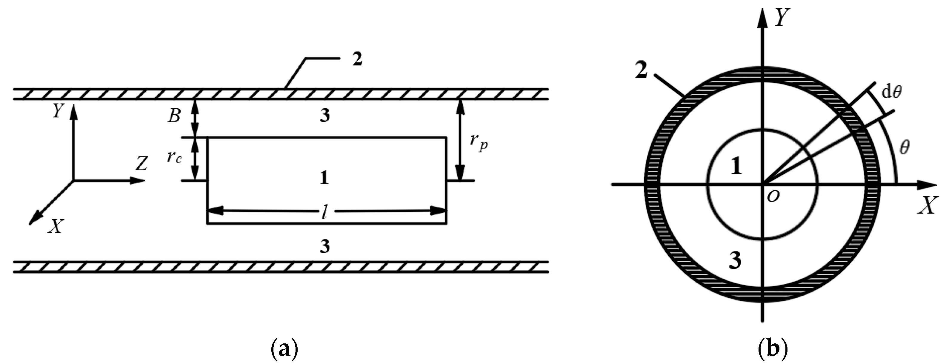
Assuming that the water flow in the annular gap is a constant flow, and ignoring the influence of the end of the pipe vehicle on the water flow in the annular gap, a three-dimensional rectangular coordinate system can be established, as shown in Figure 2.

The Navier–Stokes (N-S) equation is suitable for solving the concentric annular gap flow velocity expression. The component expressions of the N-S equation in the three-dimensional rectangular coordinate system are as follows:

$$\begin{array}{l}{F}_x-\frac{1}{\rho }\frac{\partial p}{\partial x}+\nu (\frac{{\partial }^2{u}_x}{\partial x^2}+\frac{{\partial }^2{u}_x}{\partial y^2}+\frac{{\partial }^2{u}_x}{\partial z^2})=\frac{\partial u_x}{\partial t}+(u_x\frac{\partial u_x}{\partial x}+u_y\frac{\partial u_x}{\partial y}+u_z\frac{\partial u_x}{\partial z})\\ F_y-\frac{1}{\rho }\frac{\partial p}{\partial y}+\nu (\frac{{\partial }^2{u}_y}{\partial x^2}+\frac{{\partial }^2{u}_y}{\partial y^2}+\frac{{\partial }^2{u}_y}{\partial z^2})=\frac{\partial u_y}{\partial t}+(u_x\frac{\partial u_y}{\partial x}+u_y\frac{\partial u_y}{\partial y}+u_z\frac{\partial u_y}{\partial z})\\ F_z-\frac{1}{\rho }\frac{\partial p}{\partial z}+\nu (\frac{{\partial }^2{u}_z}{\partial x^2}+\frac{{\partial }^2{u}_z}{\partial y^2}+\frac{{\partial }^2{u}_z}{\partial z^2})=\frac{\partial u_z}{\partial t}+(u_x\frac{\partial u_z}{\partial x}+u_y\frac{\partial u_z}{\partial y}+u_z\frac{\partial u_z}{\partial z})\end{array}\}$$

(1)

where F_x, F_y, F_z are the mass forces along the X, Y, and Z axes, respectively; p is the dynamic water pressure; u_x, u_y, and u_z are the fractional velocities of the annular gap flow along the X, Y, and Z axes, respectively; ν is the kinematic viscosity coefficient; and ρ is the liquid density.

For a concentric annular gap flow, it is more convenient to take the cylindrical coordinate system of the N-S equation for calculation. Equation (1), reframed in the cylindrical coordinate system, is as follows:

$$\begin{array}{l}{F}_r-\frac{1}{\rho }\frac{\partial p}{\partial r}+\nu (\frac{{\partial }^2{u}_r}{\partial r^2}+\frac{1}{r}\frac{\partial u_r}{\partial r}-\frac{u_r}{r^2}-\frac{2}{r^2}\frac{\partial u_{\theta }}{\partial \theta }+\frac{1}{r^2}\frac{{\partial }^2{u}_r}{\partial {\theta }^2}+\frac{{\partial }^2{u}_r}{\partial z^2})\\ =\frac{\partial u_r}{\partial t}+u_r\frac{\partial u_r}{\partial r}-\frac{u_{\theta }^2}{r}+\frac{u_{\theta }}{r}\frac{\partial u_r}{\partial \theta }+u_z\frac{\partial u_r}{\partial z}\\ F_{\theta }-\frac{1}{\rho r}\frac{\partial p}{\partial r}+\nu (\frac{{\partial }^2{u}_{\theta }}{\partial r^2}+\frac{1}{r}\frac{\partial u_{\theta }}{\partial r}-\frac{u_{\theta }}{r^2}+\frac{2}{r^2}\frac{\partial u_r}{\partial \theta }+\frac{1}{r^2}\frac{{\partial }^2{u}_{\theta }}{\partial {\theta }^2}+\frac{{\partial }^2{u}_{\theta }}{\partial z^2})\\ =\frac{\partial u_{\theta }}{\partial t}+u_r\frac{\partial u_{\theta }}{\partial r}-\frac{u_{\theta }{u}_r}{r}+\frac{u_{\theta }}{r}\frac{\partial u_{\theta }}{\partial \theta }+u_z\frac{\partial u_{\theta }}{\partial z}\\ F_z-\frac{1}{\rho }\frac{\partial p}{\partial z}+\nu (\frac{{\partial }^2{u}_z}{\partial r^2}+\frac{1}{r}\frac{\partial u_z}{\partial r}+\frac{1}{r^2}\frac{{\partial }^2{u}_z}{\partial {\theta }^2}+\frac{{\partial }^2{u}_z}{\partial z^2})=\frac{\partial u_z}{\partial t}+u_r\frac{\partial u_z}{\partial r}+\frac{u_{\theta }}{r}\frac{\partial u_z}{\partial \theta }+u_z\frac{\partial u_z}{\partial z}\end{array}\}$$

(2)

where F_r, F_θ, and F_z are the mass forces along the radius, the angle of θ, and the Z axis, respectively; u_r, u_θ, and u_z are the velocities along the radius, the angle of θ, and the Z axis, respectively; r = (x² + y²)^0.5; and θ = arctan(y/x).

In the concentric annular gap, the pressure dominates and the mass force can be ignored; that is, F_r = F_θ = F_z = 0. It can also be assumed that the concentric annular gap flow is a univariate flow; that is, u_r = u_θ = 0, u_z = u. Thus, Equation (2) can be simplified as follows:

$$\begin{array}{l}\frac{\partial p}{\partial r}=0\\ \frac{\partial p}{\partial \theta }=0\\ \frac{\partial p}{\partial z}=\eta (\frac{{\partial }^{2}u}{\partial r^2}+\frac{1}{r}\frac{\partial u}{\partial r}+\frac{1}{r^2}\frac{{\partial }^{2}u}{\partial {\theta }^2}+\frac{{\partial }^{2}u}{\partial z^2})\end{array}\}$$

(3)

According to Equation (3), p has nothing to do with r and θ, and is only a function of z, such that ∂p/∂z = dp/dz. Due to the symmetry of the flow on the circumference, u has nothing to do with θ, such that ∂²u/∂θ² = 0, and ∂²u/∂z² = 0 can be derived from the continuity equation. Thus, Equation (3) can be simplified to:

$$\frac{1}{\eta }\frac{\mathrm{d}p}{\mathrm{d}z}=\frac{{\partial }^{2}u}{\partial r^2}+\frac{1}{r}\frac{\partial u}{\partial r}$$

(4)

Equation (4) can be integrated as follows:

$$u=\frac{r^2}{4\eta }\frac{\mathrm{d}p}{\mathrm{d}z}+c_1\ln \mathrm{r}+c_2$$

(5)

As the two-pipe vehicles are in motion, the water flow near the body moves together with the pipe vehicle. Suppose that the moving speed of the pipe vehicle is u_c. When z = r_c, u = u_c, r = r_p, u = 0, then c₁ and c₂ can be obtained as follows:

$$\begin{array}{l}{c}_1=-\frac{u_c}{\ln r_p/r_c}-\frac{1}{4\eta }\cdot \frac{\mathrm{d}p}{\mathrm{d}z}\cdot \frac{r_p^2-r_c^2}{\ln r_p/r_c}\\ c_2=-\frac{r_p^2}{4\eta }\frac{\mathrm{d}p}{\mathrm{d}z}+\frac{u_c\ln r_p}{\ln r_p/r_c}+\frac{1}{4\eta }\cdot \frac{\mathrm{d}p}{\mathrm{d}z}\cdot \frac{r_p^2-r_c^2}{\ln r_p/r_c}\ln r_p\end{array}\}$$

(6)

The pressure gradient in the concentric annular gap obeys a linear change; that is, dp/dz = Δp/l. Then, substituting Equation (6) into Equation (5), we get:

$$u=-\frac{\Delta p}{4\eta l}{r}^2+(\frac{\Delta p}{4\eta l}\cdot \frac{r_p^2-r_c^2}{\ln r_p/r_c}-\frac{u_c}{\ln r_p/r_c})\ln r+\frac{\Delta p}{4\eta l}{r}_p^2-(\frac{\Delta p}{4\eta l}\cdot \frac{r_p^2-r_c^2}{\ln r_p/r_c}-\frac{u_c}{\ln r_p/r_c})\ln r_p{r}_c\le r\le r_p$$

(7)

Equation (7) can be simplified to:

$$u=-M{r}^2+N\ln r+M{r}_p^2-N\ln r_p$$

(8)

where M and N are calculated as follows:

$$M=\frac{\Delta p}{4\eta l}$$

(9)

$$N=\frac{\Delta p}{4\eta l}\cdot \frac{r_p^2-r_c^2}{\ln r_p/r_c}-\frac{u_c}{\ln r_p/r_c}$$

(10)

Equations (7) and (8) provide the flow velocity formula of the concentric annular gap flow when the two-pipe vehicles are moving. It can be seen from Equation (7) that when the pipe is full in the turbulent state (there is no vehicle in the pipe), different from the logarithmic distribution form, the flow velocity distribution in the concentric annular gap is parabolic. The pipeline radius r’ corresponding to the maximum flow velocity of the annular gap flow can also be calculated from Equation (7), as follows:

$$r^{\prime }=\sqrt{\frac{N}{2M}}=\sqrt{\frac{(r_p^2-r_c^2)}{2\ln (r_p/r_c)}-\frac{4\eta l{u}_c}{2\Delta p\ln (r_p/r_c)}}$$

(11)

It can be found that the maximum velocity value of the concentric annular gap flow of the pipe vehicle in the moving state is not in the middle position of the annular gap from Equation (11). The accuracy of this conclusion was verified by model experiments.

2.2. Mathematical Model of the Two-Pipe Vehicles

2.2.1. Force Analysis of the Two-Pipe Vehicles

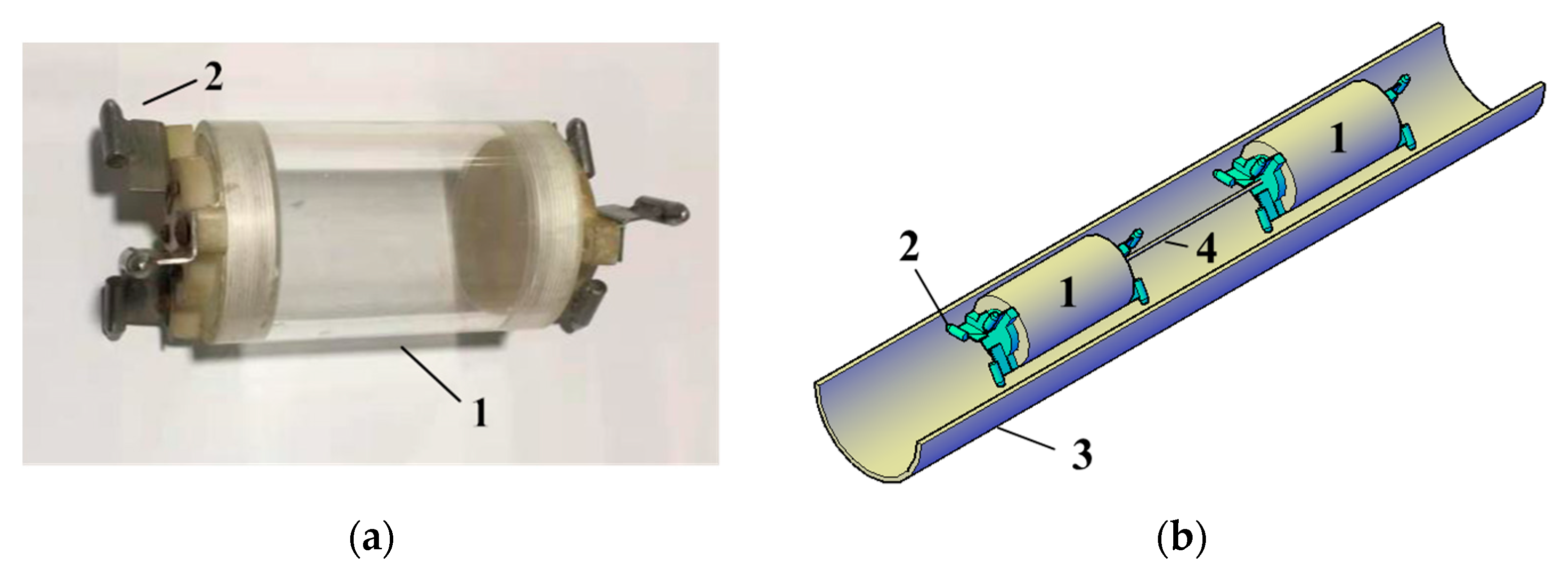
As the core component of this technology, in the simulation, the pipe vehicle is mainly composed of a barrel and some support bodies, as shown in Figure 3. The barrel is made of cylindrical plexiglass, and its interior is hollow to hold the conveyed material, thus avoiding contact between the conveyed material and the liquid in the pipe. There are supports on both ends of the barrel and three supports are arranged on each section, evenly distributed 120 degrees apart. The support body is connected to the inner wall of the pipe, such that the material barrel and the pipe are kept in a concentric state, the contact area between the material barrel and the pipe wall is reduced, and the friction between the vehicle and the pipe wall is reduced. In order to ensure that the spacing between the two pipe vehicles remains unchanged during operations, a connecting body is used to connect the vehicles. In this experiment, a spring with a wire diameter of 1 mm and an outer diameter of 5 mm was selected for the connection. The spring does not stretch or compress, has less impact on the flow field due to its spacing, and has a certain flexibility to ensure that the two-pipe vehicles can smoothly drive through curves (Figure 3).

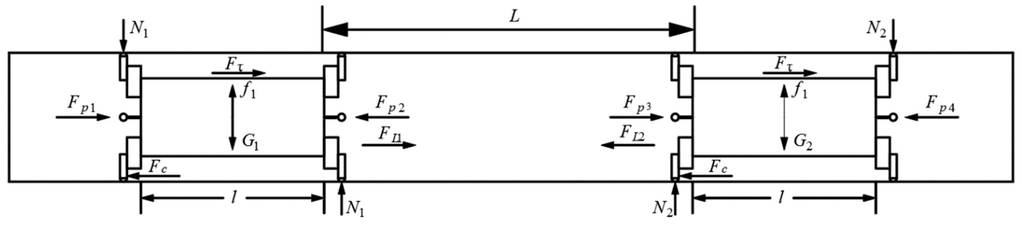
The moving speed of a two-pipe vehicles is closely related to its force. To establish the mathematical model for the movement of the two-pipe vehicles, it is necessary to first determine its force characteristics. Therefore, the force characteristics of the two-pipe vehicles during stable movement in the straight pipe section were analyzed. The force diagram for the two-pipe vehicles is shown in Figure 4.

It can be seen, from Figure 4, that a single pipe vehicle is mainly affected by seven forces. When the two-pipe vehicles are regarded as a whole, the spring force can be regarded as the internal force, such that that the two-pipe vehicles are mainly affected by six forces; namely, gravity (G), buoyancy (f), the force of the pipeline on the support body (N), the end pressure differential force (F_p), the friction force on the support body (F_f), and the shear force on the wall of the pipe vehicle (F_τ). These six forces can be divided into two directions: horizontal and vertical. Those in the vertical direction include G, f, and N. These three forces are body forces, which are mainly related to the volume of pipe vehicle and the density of conveyed materials. Those in the horizontal direction include F_p, F_f, and F_τ.

The total gravity of the two-pipe vehicles is the sum of the gravities for the rear and front vehicles, which can be expressed as follows:

$$G=G_1+G_2=2(m_w+m_c)g$$

(12)

where G₁ and G₂ represent the gravities of the rear and front vehicles, respectively; m_c is the weight of a single vehicle when it is empty; and m_w is the weight of the goods transported in a single vehicle.

As the volumes of the two pipe vehicles are exactly the same in the analysis process, the total buoyancy of the two vehicles is equal to twice the buoyancy of a single vehicle, which can be expressed as follows:

$$f=f_1+f_2=2\rho V_{c}g$$

(13)

where V_c is the volume of a single vehicle and ρ is the liquid density.

The support body of the vehicle is in contact with the wall surface. As the two-pipe vehicles move stably in the straight pipe section, the force in the vertical direction is balanced, and the supporting force N can be expressed as:

$$N=N_1+N_2=G-f$$

(14)

There is a pressure drop in the pipeline, which causes a pressure differential force on the front and rear surfaces of the pipe vehicle. This force is the main driving force for the movement of the two-pipe vehicles, which can be expressed as:

$$F_P=F_P{}_1-F_P{}_2+F_{P3}-F_{P4}=(\Delta p_1+\Delta p_2)A$$

(15)

where Δp₁ and Δp₂ denote the pressure differences between the front and rear of the two pipe vehicles, respectively, and A is the end face area of the pipe vehicle.

The support body is in contact with the wall surface of the pipeline, and a friction force will be generated during the movement of the two-pipe vehicles. The friction force calculation formula is as follows:

$$F_f=\mu N=\mu (G-f)$$

(16)

where µ is the friction coefficient.

There exists a relative motion between the water flow in the annular gap and the wall surface of the pipe vehicle, where the water flow in the annular gap will generate a shear force on the wall of the pipe vehicle. When the movement speed of the two-pipe vehicles is lower than the flow velocity of the annular gap, the shear force is the same as the movement direction of the two-pipe vehicles; that is, the shear force is the driving force. When the moving speed of the two-pipe vehicles is greater than the flow velocity of the annular gap, the shear force of the body wall is the resistance. The shear force on the wall of the pipe vehicle is as follows:

$$F_{\tau }=\frac{{\lambda }_1}{8}\rho {(v_a-v_c)}^2{A}^{\prime }$$

(17)

where λ₁ is the flow resistance coefficient, which is related to the fluid and the material of the pipe vehicle; v_a is the average velocity of the annular gap flow; v_c is the average movement speed of the two-pipe vehicles; and A’ is the sum of the side areas of the two pipe vehicles.

2.2.2. Mechanical Equilibrium Equation for Stable Movement of the Two-Pipe Vehicles

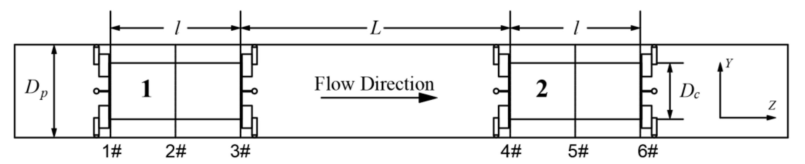
When the two-pipe vehicles move stably in a straight pipe section, it can be considered to be in a state of uniform linear motion. The space formed by the two-pipe vehicles and the pipe wall can be divided into three areas, as shown in Figure 5. Part I represents the two-pipe vehicles body area, part II represents the part of the water body area between the two pipe vehicles, and part III represents the annular gap area. When the pipe vehicle is moving at a constant speed in a straight pipeline, it can be considered that parts I and II have the same speed, such that parts I and II can be regarded as a whole.

When parts I and II are regarded as a whole, the force between these two parts can be regarded as an internal force. Parts I and II are mainly affected by four forces in the horizontal direction; namely, the pressure difference between upstream and downstream, the shear stress on the wall of the two-pipe vehicles, the friction between the two-pipe vehicles and the pipe wall, and the water flow shear stress at the interface of parts II and III. When the two-pipe vehicles are moving at a uniform speed, the force in the horizontal direction is balanced and the following relationship can be obtained, according to the force balance:

$$\frac{\Delta p\pi D_c^2}{4}+2{\tau }_1\pi D_{c}l+{\tau }_2\pi D_{c}L=F_f$$

(18)

where τ₁ is the wall shear stress of the pipe vehicle; τ₂ is the water flow shear stress at the interface of parts II and III; and Δp is the pressure difference between the upstream and downstream end faces of the pipe vehicle.

Part III is also affected by four forces in the horizontal direction; namely, the upstream and downstream pressure difference, the friction force between the pipe wall and the annular gap flow, the friction force between the two-pipe vehicles and the annular gap flow, and the water flow shear stress at the interface of parts II and III. When the two-pipe vehicles move at a uniform speed, the formula can be obtained according to the force balance, as follows:

$$\frac{\Delta p\pi (D_p^2-D_c^2)}{4}=2{\tau }_1\pi D_{c}l+{\tau }_2\pi D_{c}L+{\tau }_3\pi D_p(L+2l)$$

(19)

where τ₃ is the average shear stress at the pipe wall.

Simultaneously considering Equations (18) and (19) leads us to obtain the following equation:

$$\frac{D_c^2}{(D_p^2-D_c^2)}=\frac{F_f-2{\tau }_1\pi D_{c}l+{\tau }_2\pi D_{c}L}{2{\tau }_1\pi D_{c}l+{\tau }_2\pi D_{c}L+{\tau }_3\pi D_p(L+2l)}$$

(20)

which represents the mechanical balance equation for the stable movement of the two-pipe vehicles, providing a certain basis for the subsequent calculation of the two-pipe vehicles motion equation.

2.2.3. Motion Equation for Stable Movement of the Two-Pipe Vehicles

In Figure 5, parts I, II, and III can be regarded as a whole. According to the continuity equation, the quantity of water flowing into parts I, II, and III during the period Δt is equal to the quantity of water flowing out of these three parts, and the following relationship is obtained:

$$\rho \frac{\pi D_p^2}{4}\left(v_p-v_c\right)\Delta t=\rho \frac{\pi \left(D_p^2-D_c^2\right)}{4}\left(v_a-v_c\right)\Delta t$$

(21)

where ρ is the liquid density.

If k represents the ratio of the diameter of the pipe vehicle to the diameter of the pipe (i.e., k = D_c/D_p), then Equation (21) can be simplified to:

$$v_a=\frac{v_p-k^2{v}_c}{1-k^2}$$

(22)

τ₁ and τ₂ in Equation (18) can be expressed as follows:

$${\tau }_1=\frac{\rho {\lambda }_1(v_a-v_c{)}^2}{8}$$

(23)

$${\tau }_2=\frac{D_c}{D_p}{\tau }_3=\frac{\rho D_c{\lambda }_2{v}_a^2}{8D_p}$$

(24)

where λ₁ is the flow resistance coefficient, which is related to the fluid and the material of the pipe vehicle; and λ₂ is the friction coefficient of the pipe wall.

Substituting Equations (22)–(24) into Equation (18), we obtain the following formula:

$$\Delta P=\frac{4F_f}{\pi D_c^2}-\frac{v_p^2(2\rho {\lambda }_{1}l+\rho {\lambda }_{2}Lk)}{2k{(1-k^2)}^2{D}_p}+\frac{v_p{v}_c(2\rho {\lambda }_{1}l+\rho {\lambda }_{2}L{k}^3)}{k{(1-k^2)}^2{D}_p}-\frac{v_c^2(2\rho {\lambda }_{1}l+\rho {\lambda }_{2}L{k}^5)}{2k{(1-k^2)}^2{D}_p}$$

(25)

Let

$$E=\frac{2\rho {\lambda }_{1}l+\rho {\lambda }_{2}Lk}{2k(1-k^2{)}^2{D}_p},I=\frac{2\rho {\lambda }_{1}l+\rho {\lambda }_{2}L{k}^3}{k(1-k^2{)}^2{D}_p},J=\frac{2\rho {\lambda }_{1}l+\rho {\lambda }_{2}L{k}^5}{2k(1-k^2{)}^2{D}_p}$$

(26)

Therefore, Equation (25) can be simplified as:

$$\Delta P=\frac{4F_f}{\pi k^2{D}_p^2}-E{v}_p^2+I{v}_p{v}_c-J{v}_c^2$$

(27)

Similarly, Equation (19) can be simplified to the following form:

$$\begin{array}{c}\Delta P=\frac{v_p^2\left[2\rho k{\lambda }_{1}l+\rho {\lambda }_2(2l+L)+\rho {\lambda }_{2}L{k}^2\right]}{2(1-k^2{)}^3{D}_p}-\frac{v_p{v}_c\left[2\rho k{\lambda }_{1}l+\rho {\lambda }_2(2l+L)k^2+\rho {\lambda }_{2}L{k}^4\right]}{(1-k^2{)}^3{D}_p}\\ +\frac{v_c^2\left[2\rho k{\lambda }_{1}l+\rho {\lambda }_2(2l+L)k^4+\rho {\lambda }_{2}L{k}^6\right]}{2(1-k^2{)}^3{D}_p}\end{array}$$

(28)

Let

$$\begin{gathered} M=\frac{\left[2\rho k{\lambda }_{1}l+\rho {\lambda }_2(2l+L)+\rho {\lambda }_{2}L{k}^2\right]}{2(1-k^2{)}^3{D}_p},N=\frac{\left[2\rho k{\lambda }_{1}l+\rho {\lambda }_2(2l+L)k^2+\rho {\lambda }_{2}L{k}^4\right]}{(1-k^2{)}^3{D}_p}, \\ Q=\frac{\left[2\rho k{\lambda }_{1}l+\rho {\lambda }_2(2l+L)k^4+\rho {\lambda }_{2}L{k}^6\right]}{2(1-k^2{)}^3{D}_p} \end{gathered}$$

(29)

Therefore, Equation (28) can be simplified as:

$$\Delta P=M{v}_p^2-N{v}_p{v}_c+Q{v}_c^2$$

(30)

Simultaneously considering Equations (27) and (30), we obtain:

$$\frac{4F_f}{\pi k^2{D}_p^2}-E{v}_p^2+I{v}_p{v}_c-J{v}_c^2=M{v}_p^2-N{v}_p{v}_c+Q{v}_c^2$$

(31)

which can be simplified as follows:

$$\left(J+Q\right)v_c^2-\left(I+N\right)v_p{v}_c+\left(E+M\right)v_p^2=\frac{4F_f}{\pi k^2{D}_p^2}$$

(32)

Equation (32) is the motion equation for stable movement of the two-pipe vehicles. It can be seen that the speed of the two-pipe vehicles is related to the flow rate Q, the transport load of the two-pipe vehicles m, the spacing between the two pipe vehicles L, the diameter of the pipeline D_p, the diameter of the pipe vehicle D_c, and the vehicle length l. This formula reflects the relationship between various factors and the movement speed of the two-pipe vehicles, which can be used to qualitatively analyze the internal relationship between the movement speed of the two-pipe vehicles and each factor, providing a certain theoretical reference for optimizing the structure of two-pipe vehicles.

3. Experimental Methods

3.1. Experimental System and Procedures

The accuracy of the mathematical model was verified by designing relevant model experiments. The experimental system mainly included four parts: A power and adjustment device, a delivery and receiving device, an experimental instrument, and a conveying pipeline (see Figure 6).

(1)

The power device used in this experiment is a high-power centrifugal pump, and the adjustment device includes a control valve (gate valve) and an electromagnetic flowmeter.

(2)

The delivery device is made of trumpet-shaped stainless steel material, with a gate valve installed on the upper part, as shown in Figure 7a. The pipe vehicle starting device is installed 1.6 m downstream of the delivery device. When the pipe vehicle enters the pipeline, the starting device is in a closed state. When the pipe vehicle needs to be moved in the pipeline, the starting device is opened to release the pipe vehicle. The receiving device consists of three parts: A rectangular water tank, a baffle, and a plastic collection box, as shown in Figure 7b.

(3)

The experimental instrument mainly includes a two-pipe vehicles timing device and a flow field measurement device. The two-pipe vehicles timing device consists of an infrared probe and a display, as shown in Figure 8. Infrared probes are installed near the launching device and the outlet of the pipeline, respectively. When the two-pipe vehicles passes the first infrared probe, the timing starts, and the timing stops when it passes the second probe. According to the speed formula, the average movement speed of the two-pipe vehicles can be calculated. The flow field measurement device is a Laser Doppler Velocimeter (LDV). In order to reduce the refraction of the laser light by the pipe wall, a rectangular water jacket filled with water was added to the test pipe section.

(4)

The conveying pipe used in this test is composed of steel and plexiglass pipes. The lengths of the steel and plexiglass pipes are 8.6 m and 21.3 m, respectively, the thickness of the pipe wall is 5 mm, and the outer diameter of the pipe is 110 mm. The entire pipeline is formed by connecting multiple sections of plexiglass tubes through flanges, and a height-adjustable support body is installed at intervals below the plexiglass tubes in order to ensure that the plexiglass tubes are at the same level.

3.2. Section Selection and Measuring Point Arrangement

It was stipulated that the pipe vehicle that first comes into contact with the water flow along the direction of the water flow is the rear pipe vehicle, and the one that contacts the water flow last is the front pipe vehicle. In order to measure the three-dimensional flow velocity, a corresponding coordinate system was established in the pipeline: the water flow direction was the Z-axis, while the vertical gravity direction was the Y-axis. The corresponding X-axis was established according to the right-hand rule. Three cross-sections were arranged at the annular gap of each pipe vehicle body along the water flow direction, for a total of six sections. Then, three cross-sections were arranged at equal intervals along the length of each pipe vehicle body, for a total of six cross-sections, as shown in Figure 9.

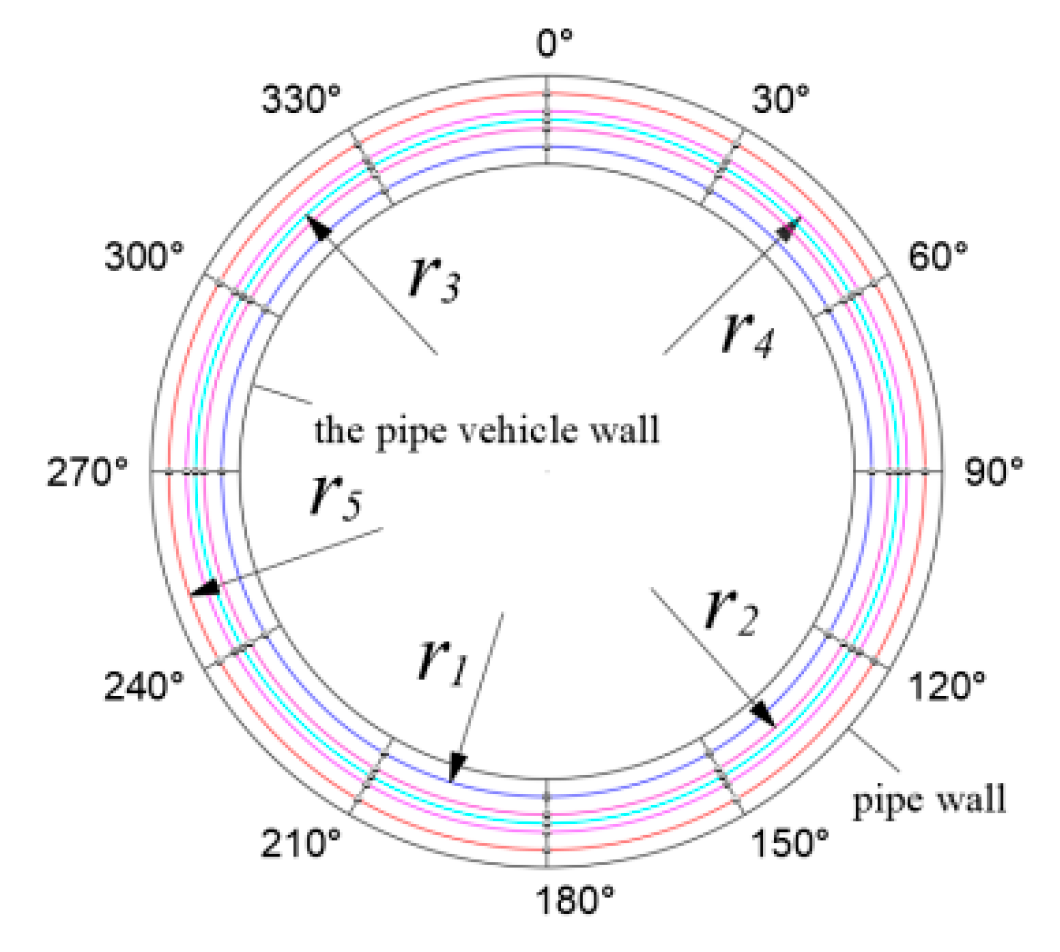
For the annular gap flow field, five measuring rings were arranged, where the measuring ring radii were r₁ = r_c + 1/5 B, r₂ = r_c + 2/5 B, r₃ = r_c + 1/2 B, r₄ = r_c + 3/5 B, and r₅ = r_c + 4/5 B (where B is the width of the annular gap). The intersection of the pipe radius and the measuring ring served as the layout measuring points, for a total of 60 measuring points, as shown in Figure 10.

3.3. Experiment Plan

From the previous analysis, it can be seen that the factors affecting the annular gap flow and the movement speed of the two-pipe vehicles mainly include the flow rate, the model of the two-pipe vehicles, the conveyed load, and the vehicle spacing. For the experiment, we adopted the principle of controlling a single variable, such that only one variable was changed in each experiment. In the experiments, the flow ratio Q was 30 m³/h, 40 m³/h, 50 m³/h, or 60 m³/h; the model dimensions of the pipe vehicle l × D_c were 150 mm × 60 mm, 150 mm × 70 mm, 150 mm × 80 mm, 100 mm × 60 mm, 100 mm × 70 mm, or 150 mm × 80 mm; the conveyed load m was 400 g, 600 g, 800 g, 1000 g, 1200 g, 1400 g, 1600 g, 1800 g, or 2000 g; and the vehicle spacing L was 7.5 cm, 15 cm, 30 cm, 45 cm, or 60 cm.

4. Results and Discussion

4.1. Mathematical Model Verification

In order to verify the accuracy of the mathematical model, taking the 2# and 5# sections as examples, the calculated and measured values of the annular gap velocity under different flow rates were compared, as shown in Figure 11.

Figure 11 shows a comparison of the calculated and measured values at the horizontal X-axis of each test section under different flow rates. It can be seen, from the figure, that the calculated and measured values under different flow rates presented a high degree of agreement, and the maximum relative error of the two calculated values did not exceed 4.58%, demonstrating the accuracy of the mathematical model. It can be seen, from the figure, that the change in flow rate did not have a significant impact on the velocity distribution of the annular gap flow. Different from the logarithmic distribution form when the pipe is full (no pipe vehicle) in the turbulent flow state, the flow velocity distribution in the concentric annular gap is seemingly parabolic. From the wall of the pipe vehicle to the wall of the pipeline, the flow velocity showed a trend of first increasing and then decreasing, and the maximum value of the flow velocity in the annular gap deviated from the middle position of the annular gap, consistent with the conclusion obtained from the previous model analysis. Different from the annular gap flow formed by the static pipe vehicle, the flow velocity was small near the vehicle body; this was because the movement of the two-pipe vehicles drove the water around the body to move together, such that the water flow near the wall surface of the pipe vehicle can obtain the same speed as the two-pipe vehicles. By comparing Figure 11a,b, it can be seen that the curve in Figure 11b changed relatively gentler; that is, the flow velocity fluctuation between the measuring points in the annular gap formed by the front pipe vehicle was smaller than that of the behind pipe vehicle, and the velocity gradient of the annular gap flow formed by the front pipe vehicle was smaller than that of the behind pipe vehicle.

Table 1. Comparison of calculated and measured values under different working conditions.

Q	l × Dc	L	m	Calculated Value	Measured Value	Relative Error
30	150 × 70	15	600	1.14	1.1	3.51
30	150 × 70	30	600	1.16	1.18	−2.01
30	150 × 70	15	1000	1.05	0.98	6.24
30	150 × 70	30	1000	1.06	1.02	3.82
30	100 × 60	15	600	1.11	1.05	5.03
30	100 × 60	45	600	1.13	1.15	−1.65
30	100 × 60	15	1000	1.01	0.96	5.29
30	100 × 60	45	1000	1.04	1.08	−4.12
50	150 × 70	15	600	1.83	1.78	2.52
50	150 × 70	45	600	1.87	1.92	−2.75
50	150 × 70	15	1000	1.67	1.68	−0.35
50	150 × 70	45	1000	1.71	1.74	−1.56
50	100 × 60	15	600	1.77	1.65	6.82
50	100 × 60	45	600	1.81	1.72	5.09
50	100 × 60	15	1000	1.62	1.51	6.99
50	100 × 60	45	1000	1.66	1.59	4.3

shows a comparison between the calculated and measured values of the two-pipe vehicles movement speeds under different working conditions.

It can be seen, from Table 1, that the maximum relative error between the calculated and measured values for the two-pipe vehicles movement speed was no more than 7%, thus verifying the accuracy of the mathematical model.

4.2. Analysis of Influencing Factors for Two-Pipe Vehicles Movement Speed

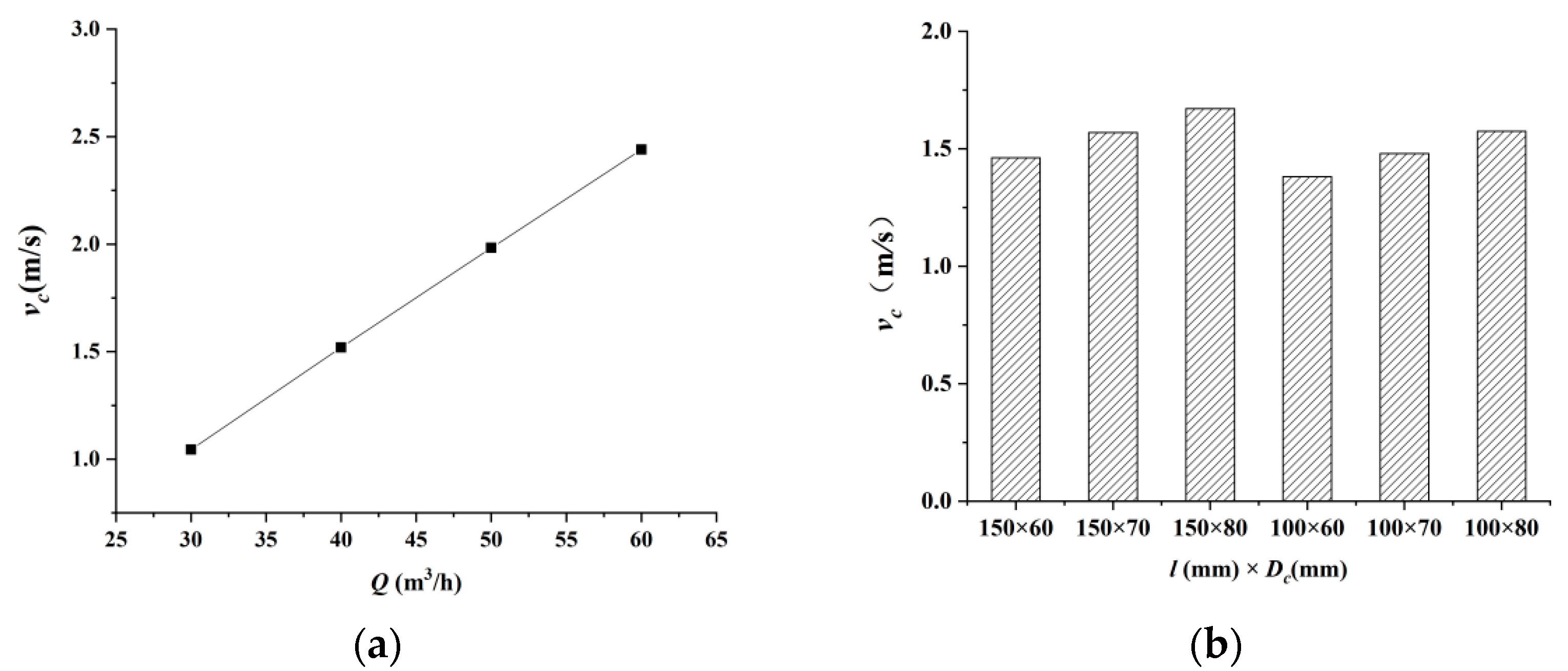
According to Equation (32), the main factors affecting the movement speed of the two-pipe vehicles are the flow rate, the vehicle model, the load, and the vehicle spacing. Therefore, the two-pipe vehicles movement speeds under different working conditions were studied respectively, as shown in Figure 12.

(1)

It can be seen, from Figure 12a, that when the other variables remained unchanged, the average movement speed of the two-pipe vehicles presented a linear relationship with the flow rate. This is mainly due to the pressure difference between the front and rear faces being the main driving force for the two-pipe vehicles. With the continuous increase in the flow rate, the differential pressure force gradually increases. Although the resistance of the pipe vehicle also gradually increases with an increase in the flow rate, the increase in the resistance with the flow rate is less than the increase in the pressure, causing the total power of the two-pipe vehicles to increase. Therefore, the movement speed of the two-pipe vehicles increases gradually with an increase in the flow rate.

(2)

It can be seen from Figure 12b that when the length of the vehicle l is held constant, the average movement speed of the two-pipe vehicles increases gradually with an increase in the diameter of the pipe vehicle D_c. This is mainly because, when the diameter D_c increases, the end face area, side wall area, and volume of the two-pipe vehicles increase accordingly. According to Equations (15)–(17), the pressure differential force and wall shear stress on the pipe vehicle gradually increase, while the frictional resistance decreases. The changes in differential pressure force, wall shear stress, and frictional resistance increase the driving force of the two-pipe vehicles, such that the movement speed of the two-pipe vehicles increases accordingly. When the diameter of the pipe vehicle is constant, the average movement speed of the two-pipe vehicles increases gradually with an increase in vehicle length. This is mainly because the longer the body length l, the larger the body side wall surface area and the body volume, such that the wall shear stress increases while the frictional resistance decreases and, so, the total driving force of the two-pipe vehicles increases. Therefore, the average movement speed of the two-pipe vehicles also increases. By comparing the experimental results, it can be seen that the average movement speed increment of the two-pipe vehicles caused by the change of diameter D_c is greater than that caused by the change in the vehicle length l.

(3)

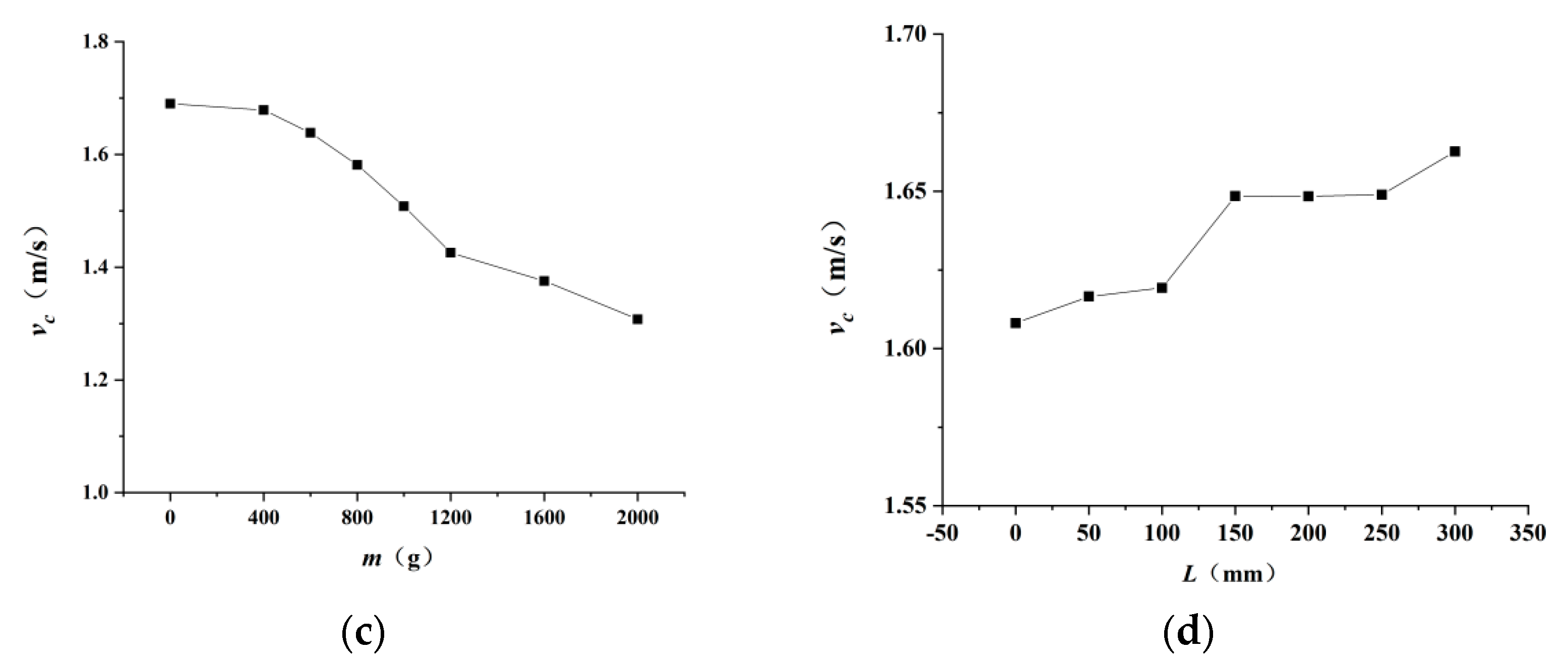
It can be seen from Figure 12c that with an increase in the conveyed load, the movement speed of the two-pipe vehicles shows a gradually decreasing trend. This is mainly due to the fact that when the model of the pipe vehicle is kept constant, the buoyancy of the two-pipe vehicles does not change; however, when the load increases, the support force of the pipe vehicle increases, and the frictional resistance increases accordingly. Therefore, the movement speed of the two-pipe vehicles is reduced.

(4)

It can be seen from Figure 12d that, with an increase in the vehicle spacing, the average movement speed of the two-pipe vehicles presents a gradually increasing trend. When the vehicle spacing is relatively small, the two-pipe vehicles can be regarded as a whole, and the pressure drop along the direction of the two-pipe vehicles is small; that is, the pressure difference between the front and rear surfaces of the two-pipe vehicles is small. With an increase in the vehicle spacing, the pressure difference between the front and rear surfaces of the pipe vehicle gradually increases and, thus, the movement speed of the two-pipe vehicles gradually increases. With a further increase in the distance between the vehicles, the influence between the two-pipe vehicles is almost negligible, and the movement speed of the two-pipe vehicles gradually changes to that of a single pipe vehicle moving in the pipeline. When the vehicle spacing reaches 300 mm, the movement of the two-pipe vehicles can basically be regarded as the movement of a single pipe vehicle. As the water flow goes through the flow process of “full pipe–annular gap–vehicle spacing–annular gap–full pipe”, when the two-pipe vehicles move in the pipeline, the energy loss is larger than that of a single pipe vehicle and the kinetic energy obtained by the two-pipe vehicles is smaller than that of a single pipe vehicle, such that the movement speed of the two-pipe vehicles is lower than that of a single pipe vehicle under the same working conditions. It can also be seen from the figure that when the spacing is between 50 mm and 150 mm, the growth rate of the average movement speed of the two-pipe vehicles is larger; that is, the slope of the curve is larger. When the spacing ratio is between 150 mm and 250 mm, the average movement speed of the two-pipe vehicles changes little with an increase in the spacing. When the spacing is greater than 250 mm, the growth rate of the average movement speed of the two-pipe vehicles becomes larger again.

It can be seen, from the above analysis, that the movement speed of the two-pipe vehicles is affected by many factors; however, the experimental results cannot comprehensively reflect the degree of influence of these factors on the movement speed. Therefore, the standard regression coefficient method in multiple regression analysis was used in order to analyze the influence degree of each factor on the speed of the two-pipe vehicles.

When dealing with the practical problems of multiple regression, the standard regression coefficient method is a method for testing the significance of the regression coefficients in multiple regression analysis. This method can eliminate the influence of the unit of the independent variable, and provides a simple and intuitive method to judge the influence degrees of multiple factors. The theory underlying this method is as follows:

Suppose a random variable Y is jointly influenced by m independent variables x₁, x₂, …, x_m, and we have a test sample size of n. Note that x_ik represents the value of the independent variable x_i in the kth trial, and Y_k represents the result of the random variable Y in the kth trial. If there exists a linear relationship between Y and x_i, the regression equation can be written as:

$$Y=a+b_1{X}_1+b_2{X}_2+\cdots +b_m{X}_m$$

(33)

The regression coefficients b_i in Equation (33) are obtained using the following equations:

$$\{\begin{array}{l}{L}_{11}{b}_1+L_{12}{b}_2+\cdots +L_{1m}{b}_m=L_{10}\\ L_{21}{b}_1+L_{22}{b}_2+\cdots +L_{2m}{b}_m=L_{20}\\ \cdots \cdots \cdots \\ L_{m1}{b}_1+L_{m2}{b}_2+\cdots +L_{mm}{b}_m=L_{m0}\end{array}$$

(34)

where

$$\begin{gathered} L_{ij}={\displaystyle \sum _{k=1}^n\left(X_{ik}-{\overline{X}}_i\right)}\left(X_{jk}-{\overline{X}}_j\right),L_{i0}={\displaystyle \sum _{k=1}^n\left(X_{ik}-{\overline{X}}_i\right)}\left(Y_k-\overline{Y}\right),L_{00}={\displaystyle \sum _{k=1}^n{\left(Y_k-\overline{Y}\right)}^2}, \\ {\overline{X}}_i=\frac{1}{n}{\displaystyle \sum _{k=1}^n{X}_{ik}},i=1,2,\cdots ,m,\overline{Y}=\frac{1}{n}{\displaystyle \sum _{k=1}^n{Y}_k} \end{gathered}$$

(35)

In order to eliminate the influence of the unit of the independent variable on the test process, we use the relationship between the standard regression coefficient b_i’ of Y to x_i and the regression coefficient b_i of Y to x_i:

$$b_i^{\prime }=b_i\sqrt{\frac{L_{ii}}{L_{00}}}$$

(36)

After calculation in Equation (36), the standard regression coefficients b_i’ has nothing to do with the units of Y and x_i, such that they can be directly compared. The larger the value of |b_i’|, the greater the effect of x_i on Y.

According to the above mathematical model, we have:

$$\{\begin{array}{c}Y=\left[v\right]\\ X=\left[D_c,l,Q,m,L\right]\end{array}$$

(37)

where D_c is 60 mm, 70 mm, or 80 mm; the pipe vehicle length l is 100 mm or 150 mm; the flow rate Q is 30 m³/h, 40 m³/h, or 50 m³/h; the conveyed load m is 400 g, 600 g, or 800 g; and the vehicle spacing L is 50 mm, 100 mm, or 150 mm. The five variables are orthogonally considered in pairs, such that the number of experiments was 162. The average movement speed of the two-pipe vehicles was obtained, according to the experimental data. Substituting the data into the corresponding equations, we obtain:

$$b_1^{\prime }=0.302\hspace{1em}{b}_2^{\prime }=0.115\hspace{1em}{b}_3^{\prime }=0.935\hspace{1em}{b}_4^{\prime }=-0.00938\hspace{1em}{b}_5^{\prime }=-7.85\times {10}^{-6}$$

(38)

According to Equation (38), we have:

$$\left|b_3^{\prime }\right|>\left|b_1^{\prime }\right|>\left|b_2^{\prime }\right|>\left|b_4^{\prime }\right|>\left|b_5^{\prime }\right|$$

(39)

Through the standard regression coefficient method, it can be seen that the influence of the flow rate Q on the movement speed of the two-pipe vehicles was the highest, followed by the diameter of the pipe vehicle D_c, the length of the pipe vehicle l, the conveyed load m, and the vehicle spacing L, in decreasing order. Therefore, in the process of transportation, it is necessary to comprehensively consider various factors to carry out reasonable matching such that the two-pipe vehicles can obtain a higher transportation movement speed.

4.3. Research Implications and Limitations

A large part of the energy loss in a two-pipe vehicles transportation system arises from the friction between the vehicle and the annular gap flow. To solve this problem, it is first necessary to understand the distribution of the annular gap flow. Therefore, in this paper, the flow velocity expression for the annular gap flow was obtained by solving the mathematical model, and its accuracy was verified through experimental tests, which can provide a theoretical reference for subsequent research on energy loss. The two-pipe vehicles motion equation obtained in this paper includes various factors affecting the movement speed, and the system designer can quickly assess the movement speed of a given two-pipe vehicles. The analysis results regarding the influence degree of each factor on the two-pipe vehicles movement speed also provide a theoretical reference for obtaining a better movement speed in the design process, as well as laying a foundation for future research on the transportation efficiency of two-pipe vehicles.

In the process of solving the annular gap flow model, the disturbance effects of the support body and the end on the annular gap flow were ignored. Therefore, whether the formula can be applied to the inlet and outlet sections of the annular gap near the support body requires further research. The mathematical model in this paper only considered the migration situation of a two-pipe vehicles in a straight pipe section; however, in practical applications, the change of terrain often leads to pipeline inclination or other problems, and whether the mathematical model is applicable in these cases still needs further research.

5. Conclusions

The mathematical model constructed in this paper includes various factors that affect the movement speed of two-pipe vehicles, and can be used to quickly calculate their movement speed. The calculated values obtained with the mathematical model were in good agreement with the experimental values. The results indicated that the concentric annular gap flow is distributed in the form of an accumulative parabola, and the maximum velocity of the flow deviated from the center of the annular gap. The movement speed of the two-pipe vehicles increased linearly with the flow Q but presented a negative linear relationship with the load m. With a gradual increase in the diameter D_c and length l of the pipe vehicle, the movement speed of the two-pipe vehicles increased gradually. With increasing spacing L, the movement speed of the two-pipe vehicles gradually increased, moving closer to that of a single vehicle. The standard regression coefficient method in the multiple regression analysis was used to analyze the influencing factors, and it was found that the flow rate Q had the strongest influence on the movement speed to the two-pipe vehicles, followed by the diameter D_c, vehicle length l, load m, and vehicle spacing L, in decreasing order.

The research results of this paper not only enrich the theory of annular gap flow at a moving boundary, but also provide a basis for further exploring the interactions between two-pipe vehicles and annular gap flows. The constructed mathematical model provides a theoretical reference for the construction and optimization of related transportation systems, as well as a theoretical basis for the realization of pipe trains in industrial applications in the near future.

References

- Mahdi, V.; Amit, K. Pipeline hydraulic transport of biomass materials: A review of experimental programs, empirical correlations, and economic assessments. Biomass Bioenergy 2015, 81, 70–82. [Google Scholar]
- Xu, H.L.; Chen, W.; Hu, W.G. Hydraulic transport flow law of natural gas hydrate pipeline under marine dynamic environment. Eng. Appl. Comp. Fluid 2020, 14, 507–521. [Google Scholar] [CrossRef]
- Vladimir, A.S. Natural Gas Pipeline Transportation as the Thermodynamic Process. J. Appl. Math. 2021, 9, 211–215. [Google Scholar]
- Umar, H.A.; Abdul Khanan, M.F.; Ogbonnaya, C.; Shiru, M.S.; Ahmad, A.; Baba, A.I. Environmental and socioeconomic impacts of pipeline transport interdiction in Niger Delta, Nigeria. Heliyon 2021, 7, e06999. [Google Scholar] [CrossRef] [PubMed]
- Hodgson, G.W.; Charles, M.E. The pipeline flow of capsules. Can. J. Chem. Eng. 1963, 42, 43–45. [Google Scholar]
- Kruyer, J.; Redberger, P.G.; Ellis, H.S. The pipeline flow of capsules. Fluid Mech. 1967, 30, 513–531. [Google Scholar] [CrossRef]
- Ismail, T.; Ulusarslan, D. Mathematical expression of pressure gradient in the flow of spherical capsule less dense than water. Int. J. Multiphas. Flow 2007, 33, 658–674. [Google Scholar]
- Brown, R.A.S. Capsule pipeline research at the Alberta Research Council. Pipeline 1987, 6, 75–82. [Google Scholar]
- Charles, M.E. Theoretical analysis of the concentric flow of cylindrical forms. Can. J. Chem. Eng. 1963, 41, 46–51. [Google Scholar]
- Ellis, H.S. An experimental investigation of the transport by water of single cylindrical and spherical capsules with density equal to that of the water. Can. J. Chem. Eng. 1964, 42, 69–76. [Google Scholar] [CrossRef]
- Kroonenberg, V.D. A Mathematical Model for Concentric Horizontal Capsule Transport. Can. J. Chem. Eng. 1978, 56, 538–543. [Google Scholar] [CrossRef]
- Latto, B.; Chow, K.W. Hydrodynamic transport of cylindrical capsules in a vertical pipeline. Can. J. Chem. Eng. 1982, 60, 713–722. [Google Scholar] [CrossRef]
- Quadrio, M.; Luchini, P. Direct numerical simulation of the turbulent flow in a pipe with annular cross section. Eur. J. Mech. 2002, 21, 413–427. [Google Scholar] [CrossRef]
- Mohamed, F.; Khalil, S.Z.; Kassab, I.G. Turbulent flow around single concentric long capsule in a pipe. Appl. Math. Model. 2009, 34, 2000–2017. [Google Scholar]
- Taimoor, A.; Mishra, R. Computational fluid dynamics based optimal design of hydraulic capsule pipelines transporting cylindrical capsules. Powder Technol. 2016, 295, 180–201. [Google Scholar]
- Lenau, C.W. Unsteady Flow in Hydraulic Capsule Pipeline. J. Eng. Mech. 1996, 122, 1168–1173. [Google Scholar] [CrossRef]
- Vlasak, P. An experimental investigation of capsules of anomalous shape conveyed by liquid in a pipe. Powder Technol. 1999, 104, 207–213. [Google Scholar] [CrossRef]
- Khalil, M.F.; Hammoud, A.H. Experimental investigation of hydraulic capsule pipeline with drag reducing surfactant. In Proceedings of the 8th International Congress of Fluid Dynamics and Propulsion, Sharm El-Sheikh, Sinai, Egypt, 14–17 December 2006. [Google Scholar]
- Huang, X.; Liu, H.; Thomas, R.M. Polymer drag reduction in hydraulic capsule pipeline. AIChE J. 1997, 43, 1117–1121. [Google Scholar] [CrossRef]
- Taimoor, A.; Abdualmagid, A.; Rakesh, M. Effect of capsule shape on hydrodynamic characteristics and optimal design of hydraulic capsule pipelines. J. Petrol. Sci. Eng. 2018, 161, 390–408. [Google Scholar]
- Swamee, P.K. Design of sediment transporting pipeline. J. Hydraul. Eng. 1995, 121, 72–76. [Google Scholar] [CrossRef]
- Li, Y.Y.; Sun, Y.H. Mathematical Model of the Piped Vehicle Motion in Piped Hydraulic Transportation of Tube-Contained Raw Material. Math. Probl. Eng. 2019, 2019, 3930691. [Google Scholar] [CrossRef]
- Zhang, X.L.; Sun, X.H.; Li, Y.Y. 3-D numerical investigation of the wall-bounded concentric annulus flow around a cylindrical body with a special array of cylinders. J. Hydrodyn. 2015, 27, 120–130. [Google Scholar] [CrossRef]
- Xiao, N.Y.; Ma, J.J.; Li, Y.Y. Wall Stresses in Cylinder of Stationary Piped Carriage Using COMSOL Multiphysics. Water 2019, 11, 1910. [Google Scholar]
- Xiao, N.Y.; Ma, J.J. The Wall Stress of the Capsule Surface in the Straight Pipe. Water 2020, 12, 242. [Google Scholar]
- Jia, X.M.; Sun, X.H.; Song, J.R. Effect of Concentric Annular Gap Flow on Wall Shear Stress of Stationary Cylinder Pipe Vehicle under Different Reynolds Numbers. Math. Probl. Eng. 2020, 2020, 1253652. [Google Scholar] [CrossRef]
- Zhang, C.J.; Sun, X.H.; Li, Y.Y. Effects of Guide Vane Placement Angle on Hydraulic Characteristics of Flow Field and Optimal Design of Hydraulic Capsule Pipelines. Water 2018, 10, 1378. [Google Scholar] [CrossRef]
- Wang, J.; Sun, X.H.; Li, Y.Y. Analysis of Pressure Characteristics of Tube-Contained Raw Material Pipeline Hydraulic Transportation under Different Discharges. In Proceedings of the International Conference on Electrical, Mechanical and Industrial Engineering (ICEMIE), Phuket, Thailand, 24–25 April 2016; pp. 44–46. [Google Scholar]
- Zhang, C.J.; Sun, X.H.; Li, Y.Y. Hydraulic Characteristics of Transporting a Piped Carriage in a Horizontal Pipe Based on the Bidirectional Fluid-Structure Interaction. Math. Probl. Eng. 2018, 2018, 8317843. [Google Scholar] [CrossRef]
- Ulusarslan, D.; Ismail, T. An experimental investigation of the capsule velocity, concentration rate and the spacing between the capsules for spherical capsule train flow in a horizontal circular pipe. Powder Technol. 2005, 159, 27–34. [Google Scholar] [CrossRef]
- Ulusarslan, D.; Ismail, T. An experimental determination of pressure drops in the flow of low density spherical capsule train inside horizontal pipes. Exp Therm Fluid Sci. 2005, 30, 233–241. [Google Scholar] [CrossRef]
- Alam, M.M. Lift Forces Induced by the Phase Lag between the Vortex Sheddings from Two Tandem Bluff. Bodies. J. Fluid Struct. 2016, 65, 217–237. [Google Scholar] [CrossRef]
- Carmo, B.S.; Meneghini, J.R. Numerical investigation of the flow around two circular cylinders in tandem. J. Fluids Struct. 2006, 22, 979–988. [Google Scholar] [CrossRef]
- Taimoor, A.; Mishra, R. Optimal design of hydraulic capsule pipeline transporting spherical capsules. Can. J. Chem. Eng. 2016, 94, 966–979. [Google Scholar]
- Taimoor, A.; Mishra, R. Development of a design methodology for hydraulic pipelines carrying rectangular capsules. Int. J. Press. Ves. Pip. 2016, 146, 111–128. [Google Scholar]
Figure 1.
Pipe side view. Note: 1. pipe vehicle; 2. Support body; 3. Pipeline; and 4. Concentric annular gap.
Figure 2.
Three-dimensional rectangular coordinate system: (a) Sectional view; and (b) Side view. Note: 1. Pipe vehicle; 2. Pipe wall; 3. Concentric annular gap; l represents the length of the pipe vehicle, rp represents the pipe radius, rc represents the pipe vehicle radius, and B represents the width of the annular gap.
Figure 3.
Structure diagram of the two-pipe vehicles: (a) A single vehicle; and (b) Two-pipe vehicle. Note: 1. Barrel; 2. Support body; 3. Pipeline; 4. Linker.
Figure 4.
Force diagram of a two-pipe vehicles. Note: G1, G2 are gravity; f1, f2 are buoyancy; N1, N2 are the force of the pipeline on the support body; Fp1, Fp2, Fp3, Fp4 are the end pressure differential force; Ff1, Ff2 are the friction force on the support body; Fτ1, Fτ2 are shear force on the wall of the pipe vehicle; FL1, FL2 are the spring force.
Figure 5.
Schematic diagram of area division. Note: Dc is the diameter of the vehicle, Dp is the diameter of the pipe, va is the velocity of the annular gap flow, vc is the movement speed of the two-pipe vehicles, and vp is the water flow velocity in the pipe.
Figure 6.
Experimental system. Note: 1. Centrifugal pump. 2. Regulating valve. 3. Electromagnetic flowmeter. 4. Feeding device. 5. Brake device. 6. Infrared probe. 7. timer. 8. Pressure sensors. 9. Rectangular water jacket. 10. Laser Doppler velocimeter. 11. Laser probe. 12. Computer. 13. Water tank.
Figure 7.
Delivery and receiving devices: (a) Delivery device; and (b) receiving device.
Figure 8.
Timing device for the two-pipe vehicles.
Figure 9.
Layout of the measuring cross-sections. Note: 1. Rear pipe vehicle; 2. Front pipe vehicle.
Figure 10.
Schematic of measuring point layout.
Figure 11.
Comparison of calculated and measured values: (a) 2# cross-section; and (b) 5# cross-section.
Figure 12.
Two-pipe vehicles movement speed under different working conditions: (a) Under different flow rates; (b) under different vehicle models; (c) under different loads; and (d) under different vehicle spacings.