Long-Term Trend and Inter-Annual Variation of Ocean Heat Content in the Bohai, Yellow, and East China Seas

Abstract

The long-term trend and interannual variation of ocean heat content (OHC) in the Bohai Sea, Yellow Sea, and East China Sea (BYECS) were examined using 27 years (1993–2019) of daily reanalysis data from the Japan Coastal Ocean Predictability Experiment 2 (JCOPE2M). The annual mean OHC was 4.25 × 10²¹ J, with a linear warming rate of 0.13 W m⁻² with a confidence level of 95%. The spatial distributions for the annual and linear trends of OHC in the BYECS were inhomogeneous, and a considerable quantity of heat was stored on the outer shelf. The warming rate was considerably elevated in the areas northeast of Taiwan and southwest of Kyushu, showing a rate greater than that of the Pacific and global oceans by a factor of 4–5. Heat budget analysis indicated that the Taiwan Strait (TAS) is the dominant source of heat for the BYECS. The mechanisms of the OHC interannual variation in the outer and inner shelves varied. On the outer shelf, the OHC interannual variation was dependent on the Kuroshio onshore intrusion, while on the inner shelf, the OHC interannual variation was related to the variation in air-sea heat flux. The rapid warming in the outer shelf corresponded to the increasing trends of heat transport across northeast Taiwan and southwest Kyushu, which were dominated by the temporal variation of current velocity.

1. Introduction

As a heat reservoir, the global ocean accumulates excess heat as a result of greenhouse gas emissions from anthropogenic activities [1]. The global ocean heat content (OHC) indicates mean warming at a rate of 0.35 W m⁻² from 1955 to 2019. This rate is averaged over the global oceanic surface, and the mean rate since 1990 has increased to approximately 0.61 W m⁻² [1,2,3]. Despite the rapid warming of the global ocean surface, the OHC warming rate has never been observed to be spatially uniform. The western boundary current regions have been reported to have a particularly elevated warming rate [4,5,6]. Specifically, marginal seas, which are highly sensitive to climate change, show a much greater warming rate than open oceans [7,8]. The Sea of Japan, a marginal sea in the northwest Pacific Ocean, for example, was observed to have a mean OHC warming rate that was two times that of the Pacific Ocean from 1976 to 2007 [5].

The Eastern China Seas, which include the East China Sea (ECS), the Yellow Sea, and the Bohai Sea, also marginal seas located in the northwest Pacific Ocean are bound by the 200 m isobaths (BYECS, Figure 1). The ECS has also been observed to have a warming trend during the last century [9,10]. Long-term sea surface temperature (SST) data have been widely used to examine the rapid ECS warming [11,12,13]. The mechanism responsible for the SST rise in the ECS was examined using both observational and reanalysis data. The warming SST has been demonstrated to be controlled by an increase in ocean advection and local atmospheric forcing [10,13,14,15].

Compared to SST data, OHC data indicate a larger signal-to-noise ratio and are less influenced by natural variability [16]. OHC is more suitable for investigating the temporal variation of ocean warming over the water column than SST [1,17]. However, few studies have focused on OHC on the BYECS shelf [18]. To analyze the OHC budget and the cause for its variation, a combined assessment of the heat transport from both the lateral boundaries and the air-sea heat fluxes were required.

The change of OHC in the BYECS is determined by heat transport through the lateral boundaries and air-sea heat flux [19,20]. As for the lateral boundaries, the BYECS exchanges heat with the surrounding seas principally through the shelf-break section (SBS, usually defined by the 200 m isobaths), Taiwan Strait (TAS), and Tsushima Strait (TUS). Along the SBS, water exchange between the Kuroshio and shelf was responsible for a substantial portion of the heat transport. The Kuroshio Current enters the ECS from the East Taiwan Channel (Figure 1) and intrudes onto the ECS shelf, mainly in the northeast of Taiwan and southwest of Kyushu [21,22]. Warm water from the South China Sea is also transported into the ECS through the TAS, and eventually, the Tsushima warm current envelops this external water and heat from the BYECS to the Sea of Japan through the TUS. The water exchange between the ECS and the surrounding seas through these three sections has been discussed [21,23,24], and some studies have evaluated heat transport [25,26]. Using a global ocean model, Liu et al. [25] reported that the time-averaged heat transport through the TAS, TUS, and SBS was 2 × 10¹⁴, 2.1 × 10¹⁴, and 0.5 × 10¹⁴ W, respectively. In addition, the heat transport into the ECS also showed interannual variations [27], which potentially regulated the interannual variation of OHC in the ECS.

To better understand warming in the ECS, the OHC, and BYECS shelf heat budgets were calculated using the Japan Coastal Ocean Predictability Experiment 2 (JCOPE2M) reanalysis data. The interannual variation and warming trend of the BYECS from 1993 to 2019 were discussed from the perspective of OHC.

2. Materials and Methods

2.1. JCOPE2M Reanalysis Data

In this study, daily hydrodynamic data were obtained from JCOPE2M, which is operated by the Japan Agency for Marine-Earth Science and Technology (JAMSTEC). This model, based on the Princeton Ocean Model with a generalized sigma coordinate (POMgcs) [28], is a three-dimensional, eddy-resolving, and data-assimilative ocean model. The model domain covers the Northwest Pacific (10.5–62° N, 108–180° E) with a horizontal resolution of 1/12° for meridional and zonal directions and a vertical resolution of 47 sigma layers, which could reproduce the Kuroshio, a strong western boundary current in the northwestern Pacific. The bottom topography is from 1/12° global height data, referred to as GETECH DTM5, with an additional boundary condition for which the minimum and maximum depths are 10 m and 6500 m, respectively. Notably, the 1/12° bottom topography data used by Uehara et al. [29] are embedded in the Eastern China Seas.

The JCOPE2M model was driven by the atmospheric forcing of wind stresses, heat, and salt fluxes at the sea surface. The wind stress and heat flux fields were calculated from 6-hourly National Centers for Environmental Prediction/National Center for Atmospheric Research (NCEP/NCAR) reanalysis data using bulk formulas [30,31]. The merged satellite and in-situ global daily SST (MGDSST) data were employed for surface heat flux correction. The salinity at the surface was restored to the monthly mean climatology data on a 30-day timescale after importing precipitation and evaporation data from the NCEP/NCAR reanalysis data. Using the one-way nesting method [32], the lateral boundary condition of this model was determined by an outer model, which has a 1/4° horizontal resolution and 21 sigma levels in the vertical direction. It encompasses almost the entire North Pacific Ocean (30° S–62° N, 100° E–90° W). Sea surface temperature data from remote sensing and temperature/salinity profiles from in situ observations were assimilated into the JCOPE2M model through the multi-scale three-dimensional variational scheme method. This method promises effective simulation of ocean conditions in the western North Pacific. Notably, there is no assimilation of in-situ profiles in the shelf region of the BYECS [33].

The JCOPE2M and its outer model were spun up for 5 and 15 years, respectively. Reanalysis calculations from November 1992 were performed for both models using data assimilation and external forcing. More details on the model parameters are described by Miyazawa et al. [33,34]. In this study, the daily mean water temperature, salinity, and two horizontal velocity components from 1993 to 2019 were provided for the following analysis.

2.2. Methods

2.2.1. Calculating the OHC

The OHC in the BYECS is vertically integrated from the sea surface to the sea bottom, as follows:

$$\mathrm{OHC}={{\displaystyle \int }}_{-H}^0{c}_p\rho \left(x,y,z\right)t\left(x,y,z\right)dz$$

(1)

where H is the maximum water depth at each grid point, cp = 3996 J kg⁻¹ °C⁻¹ is the specific heat capacity of seawater, and $\rho$ (kg m⁻³) and $t$ (°C) are the potential density and temperature of seawater, respectively. The terms x and y are the horizontal coordinates and z is the vertical coordinate. dz is the vertical interval of the grid points. After obtaining the OHC in each grid point, the total OHC (OHC_T) in the BYECS is then calculated by an area integral of OHC.

The change in the total OHC over the BYECS (OHC_T) is defined as the sum of the air-sea heat flux (Q_N) and heat transport through the lateral boundaries (Q_V):

$$\frac{\partial OH{C}_T}{\partial \mathrm{t}}=-Q_N+Q_V$$

(2)

2.2.2. Calculating the Heat Transport

Heat exchange in the BYECS with the surrounding seas mainly occurs through the SBS, TAS, and TUS (black lines in Figure 1). The inflow heat transport (IHT), outflow heat transport (OHT), and net heat transport (NHT) were calculated as follows:

$$\mathrm{IHT}=\iint c_p\rho \left(x,y,z\right)t\left(x,z\right)v_{+}\left(x,z\right)dxdz$$

(3)

$$\mathrm{OHT}=\iint c_p\rho \left(x,y,z\right)t\left(x,z\right)v_{-}\left(x,z\right)dxdz$$

(4)

$$\mathrm{NHT}=\iint c_p\rho \left(x,y,z\right)t\left(x,z\right)v\left(x,z\right)dxdz$$

(5)

where dx is the horizontal interval of the grid points, v is the monthly velocity component normal to the sections, v+ and v− denote the onshore and offshore directions, respectively.

2.2.3. Exacting the Interannual Signal

To characterize the interannual time series of OHC, the heat transport through the lateral boundaries, and the air-sea heat flux, the following steps were conducted on the original daily data: (1) the daily variables were averaged to obtain a monthly-mean time series; (2) the anomalies observed in these monthly mean data were obtained by subtracting the annual mean values; (3) the seasonal variations were removed from the monthly anomalies by subtracting the climatological monthly mean values; (4) the linear trend, as captured using least squares method, was removed from the monthly anomalies; and finally, (5) the intraseasonal variations were removed from the monthly perturbations by applying a 13-month running mean. The resultant single interannual variations for the original time series were utilized for subsequent analysis.

3. Results and Discussion

3.1. Model Validation

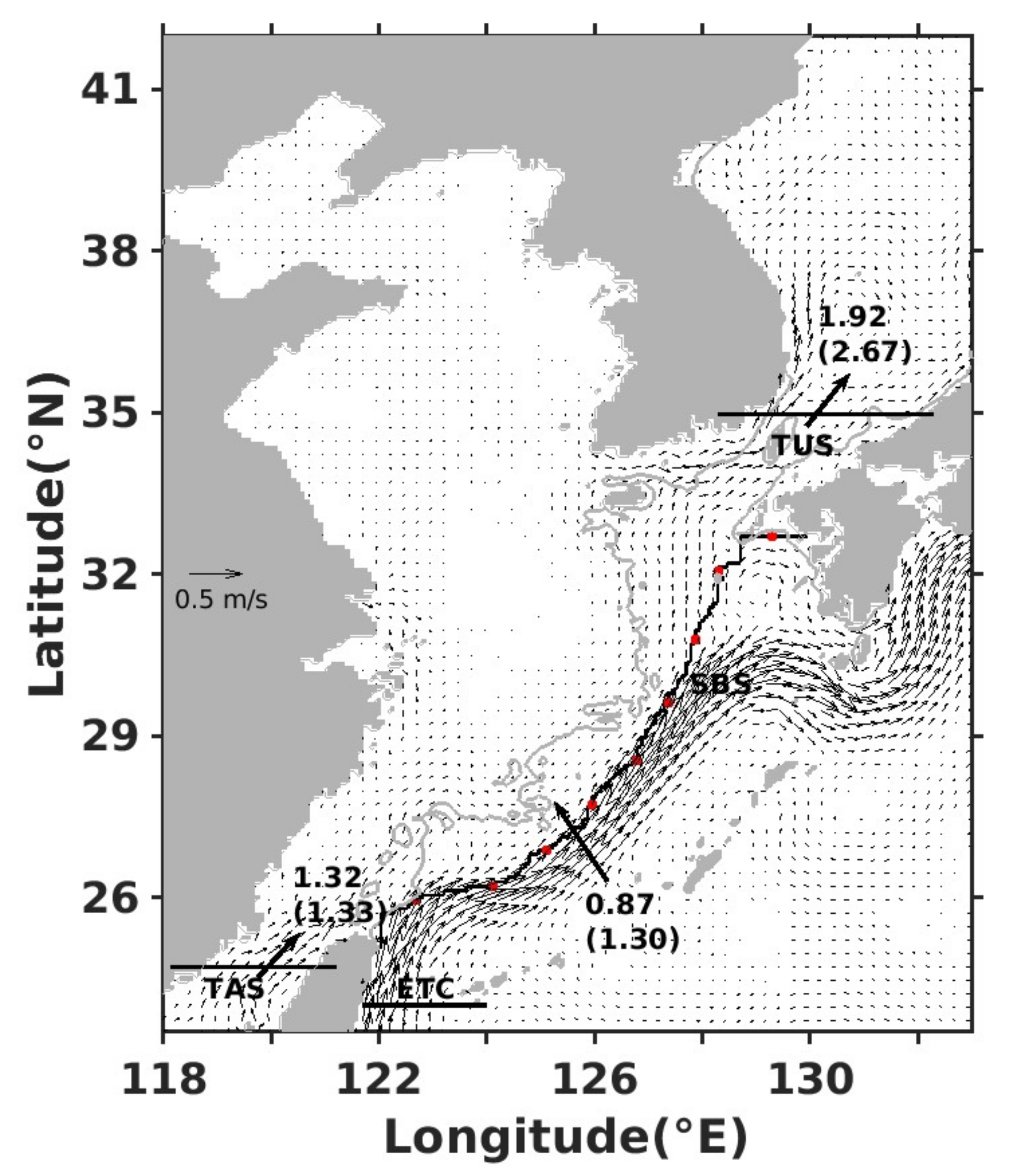
The BYECS study area is shown in Figure 1. The annual mean current at the sea surface showed a marked contrast in spatial distribution. The Kuroshio Current, with a velocity of ~1 m s⁻¹, enters the ECS from the east of Taiwan, and the main flow turns northeastward and flows along the 200 m isobaths (black curve line in Figure 1), veers east around 30° N, 129° E, and finally exits the ECS through the Tokara Strait. Meanwhile, the nearshore Kuroshio branch intrudes onshore via the 200 m isobaths and soon returns to the Kuroshio mainstream. The Kuroshio Current transports large amounts of warm water from low latitudes and contributes considerably to the BYECS heating process. Furthermore, currents such as the Taiwan Strait Current, China Coastal Current, and Tsushima Warm Current can also be identified in the distribution of surface currents.

The validation of the current velocity from the JCOPE2M was performed by comparing the data on annual mean volume transport through the SBS, TAS, and TUS with those observed in previous studies (

Table 1. Comparison of long-term averaged transport through the SBS, TAS, and TUS observed in previous studies and modelled by the JCOPE2M.

	Model/Sv	Obs./Sv	References
Shelf break section	1.3	1.4	[35]
Tsushima Strait	2.67	2.3–2.7	[36]
		2.64	[37]
		2.65	[38]
Taiwan Strait	1.33	1.8	[39]
		1.2	[35]

). In the JCOPE2M model, the annual mean net volume transport was 1.33, 1.30, and 2.67 Sv through the TAS, SBS, and TUS, respectively. The negligible discrepancy with the observations confirms the reliability of the JCOPE2M results for the mean-state transport.

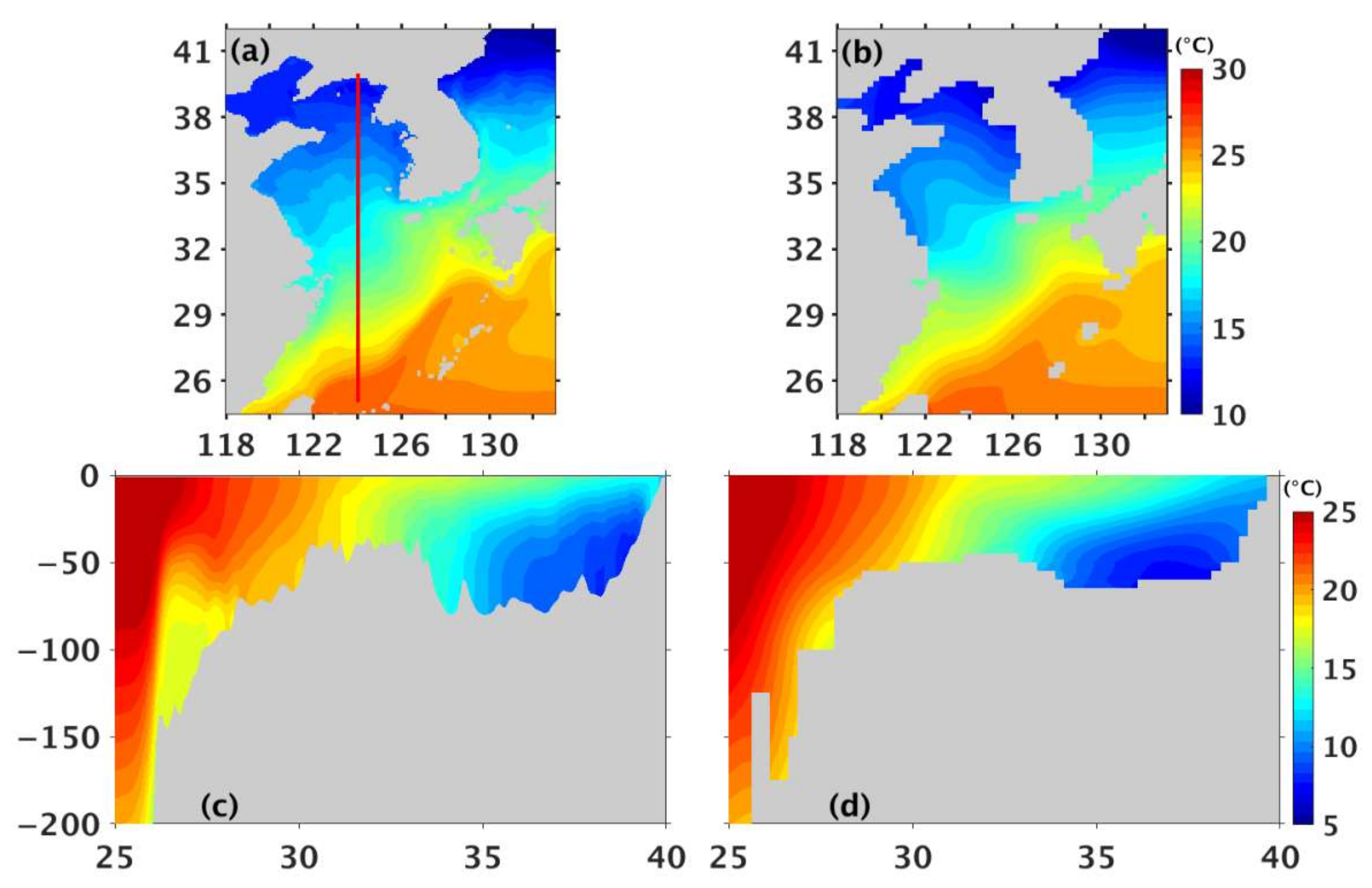
We compared the annual mean seawater temperature in the BYECS from JCOPE2M reanalysis data with WOA2018 data [40], which collected the temperature based on profile data from the World Ocean Database, at both the sea surface and 124° E section (Figure 2). The JCOPE2M model was skilled at capturing the basic features of the observations of SST and vertical distribution. The SST was higher in the southeast of the BYECS and decreased toward the northwest region (Figure 2a,b). The intrusions of warm water from northeast Taiwan and southwest Kyushu in the observations can also be found in the model results. The vertical profile in both models and observations indicated an elevated temperature from the sea surface to a depth of −200 m in the Kuroshio mainstream at 25° N, and upward cold water from the bottom at 27° N and north of 35° N (Figure 2c,d).

3.2. Spatial Distribution of OHC in the BYECS

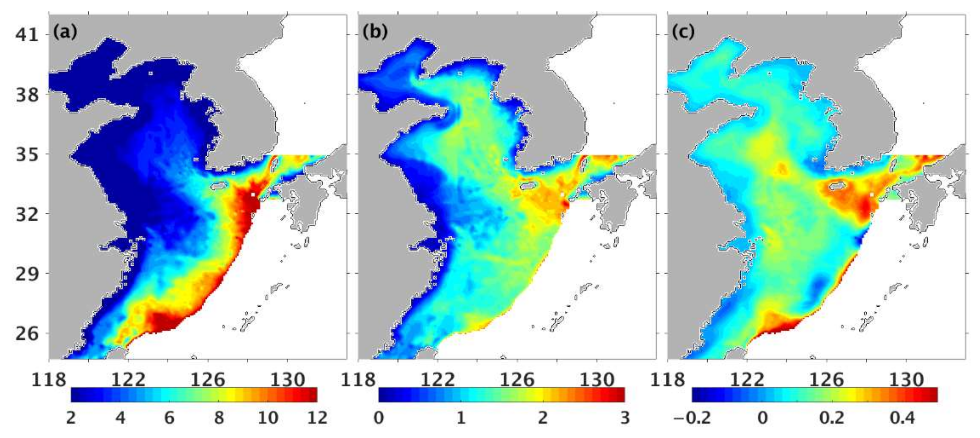
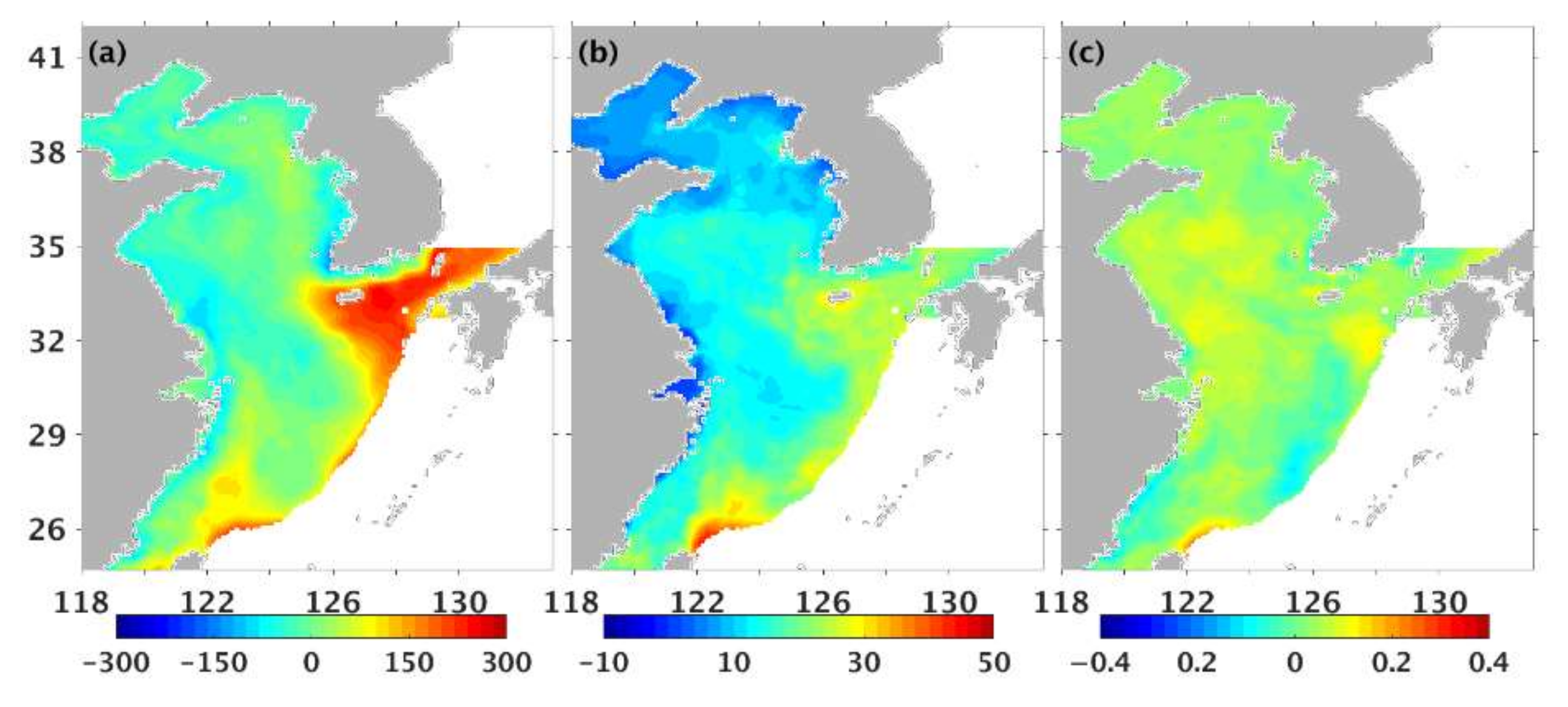
Based on the JCOPE2M reanalysis data, the annual mean (1993–2019) OHC over the BYECS shelf is 4.25 × 10²¹ J. Figure 3a,b show the annual mean and standard deviation for the OHC in the upper 200 m of the BYECS. The spatial pattern of OHC was not uniform over the BYECS, and the OHC in the southeastern BYECS was greater than that in the inner shelf by at least one order of magnitude. The maximum OHC was principally found in areas northeast of Taiwan and southwest of Kyushu, which are the two main pathways for Kuroshio intrusion over the shelf [21,22]. The distribution of the standard deviation was similar to the annual mean OHC, indicating a larger interannual fluctuation in the region where the Kuroshio onshore intrusions occurred.

To examine the results from the JCOPE2M analysis data, the OHC in the BYECS shelf was also calculated by another reanalysis data from 1993 to 2015, the FORA-WNP30 (http://synthesis.jamstec.go.jp/FORA/index.html, accessed on 11 March 2020), with a horizontal resolution of 1/10°. The annual mean OHC over the shelf was 3.93 × 10²¹ J, and the spatial distribution of OHC in the BYECS shelf from the FORA data was similar to that from the JCOPE2M data (the figures were not shown).

Figure 3c showed the linear trend of OHC in the BYECS shelf from 1993 to 2019, and the annual mean warming trend was 0.13 W m⁻² with a confidence level of 95%. The OHC warming trend in the BYECS shelf from the FORA data (1993–2015) was 0.24 W m⁻², which was about twice the warming rate calculated by the JCOPE2M. The linear trend in the BYECS was slightly smaller than that of the global ocean OHC during 1990–2019 (0.61 W m⁻², Garcia-Soto, et al. [1]).

The spatial pattern for the linear trend indicates inhomogeneous warming and cooling change in the shelf. The trend showed a positive value in a wide region of the shelf, especially in regions northeast of Taiwan and southwest of Kyushu. The maximum warming rate was about 0.93 W m⁻², which was approximately greater than that of the Pacific and global oceans by a factor of 4–5. In addition, the OHC also has an elevated warming trend in the central Yellow Sea and to the east of the Yangtze River estuary. The associated warming rate was approximately greater than that of the Bohai Sea by a factor of three. However, the OHC in the middle of the 200 m isobaths showed a cooling trend, although the cooling rate was less than the warming rate in the areas northeast of Taiwan and southwest of Kyushu.

3.3. OHC Heat Budget

3.3.1. Heat Transport across the Lateral Boundaries

The annual mean heat transports are 1.32 × 10¹⁴, 0.87 × 10¹⁴, and −1.92 × 10¹⁴ W across the TAS, SBS, and TUS, respectively (Figure 1). The heat transfer by the TAS contributed more heat to the shelf than the SBS. A previous study showed a similar annual mean strength of heat transport from 1980–2009 was found across the SBS (1.23 × 10¹⁴ W) and TUS (−1.8 × 10¹⁴ W) in the results based on the ROMS ocean model, but the heat transport (0.82 ×10 ¹⁴ W) through the TAS was smaller than that across the SBS [41], which was reversed in this study.

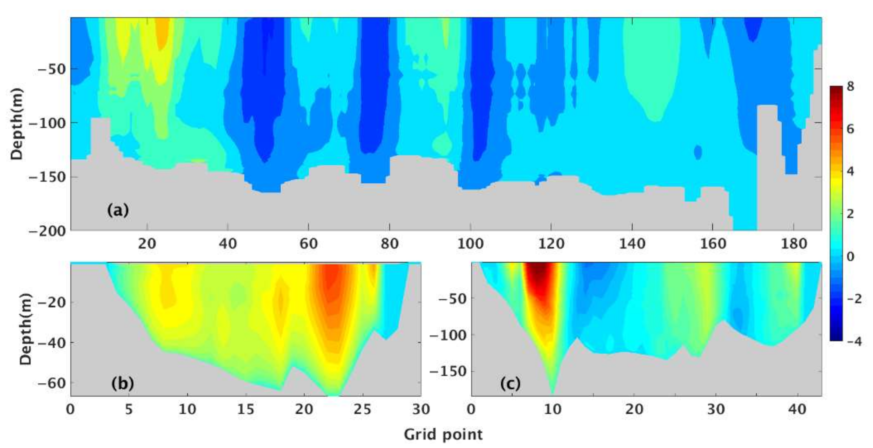
The SBS followed the 200 m isobaths. The grid point numbers were provided as horizontal coordinates. The vertical variation in heat transport across the SBS was smaller than that in the horizontal direction (Figure 4a), which was similar to the velocity distribution at these grid points [24]. The heat transport was from the onshore direction from the sea surface to the bottom at grid points 5–40, 80–100, and 135–160 but in the offshore direction at gird points 42–56, 70–80, and 160–180. These three onshore intrusion locations have been reported by previous research [22,24,32]. The remarkable heat intrusion occurred in the upper 50 m in the northeast of Taiwan (grid point 5–40) with a maximum onshore velocity greater than 20 cm s⁻¹. This was followed by onshore intrusion in the area southwest of Kyushu (grid point 135–160) and the middle of the shelf break (grid point 80–100).

The heat transport vertical structure from the TAS was uniform, the northward transport mainly occurred to the east of the TAS (grid point 20–25, Figure 4b), and the magnitude of the heat transport was greater than that in the northeast of Taiwan along the SBS. The total net heat transport through the TAS was also greater than that through the SBS owing to the offshore heat transport from the shelf to the open ocean across the SBS in some water columns.

Heat loss originating from the TUS occurred mainly in the western channel of the TUS (Figure 4c). The strength of the western intrusion across the TUS was significant, and the net heat loss from the TUS was approximately twice that of the onshore intrusion through the SBS.

3.3.2. Air-Sea Heat Exchange

The air-sea heat flux (Q_N) is the sum of shortwave radiation, longwave back radiation, and sensible and latent heat fluxes. As an external heat source, Q_N also modulates the OHC of the BYECS through heat exchange over the air-sea interface. The annual mean air-sea heat flux in the BYECS calculated from the JCOPE2M is −0.22 × 10¹⁴ W, indicating heat transfer from the BYECS to air. Figure 5a presents the annual mean (1993–2019) air-sea heat flux from the JCOPE2M reanalysis data. Q_N is positive for almost the entire BYECS, which indicates net heat loss from the BYECS to the atmosphere on the mean-state timescale. The net heat loss was especially remarkable in areas northeast of Taiwan and southwest of Kyushu, which was balanced by the heat gain from the Kuroshio onshore intrusion. The annual mean standard deviation was also elevated in these two regions (Figure 5b).

Figure 5c shows the linear trend for the air-sea heat flux on the BYECS shelf from 1993 to 2019. The spatial pattern of the linear trend had many positive values, which indicated a heat loss trend for the majority of the BYECS shelf. Air-sea heat exchange in areas northeast of Taiwan and southwest of Kyushu indicated a rapid heat loss trend but showed a sow heat loss trend in the middle of the SBS. In addition, a downward heat gain of the air-sea heat flux was observed in the central Yellow Sea. The distribution of the linear trend of the air-sea heat flux was similar to the linear OHC trend.

The ocean currents through the three lateral boundaries contribute to a net heat gain for the BYECS, which are balanced by the upward air-sea flux. According to Equation (2), the OHC tendency was dominated by the air-sea heat flux (Q_N) and meridional transport of ocean currents (Q_V). The net heat loss from air-sea exchange and the net heat gain from ocean currents was of the same order of magnitude. The difference between the heat transferred by each mechanism was less than the annual mean OHC by two orders of magnitude.

3.4. Interannual OHC Variation in the BYECS

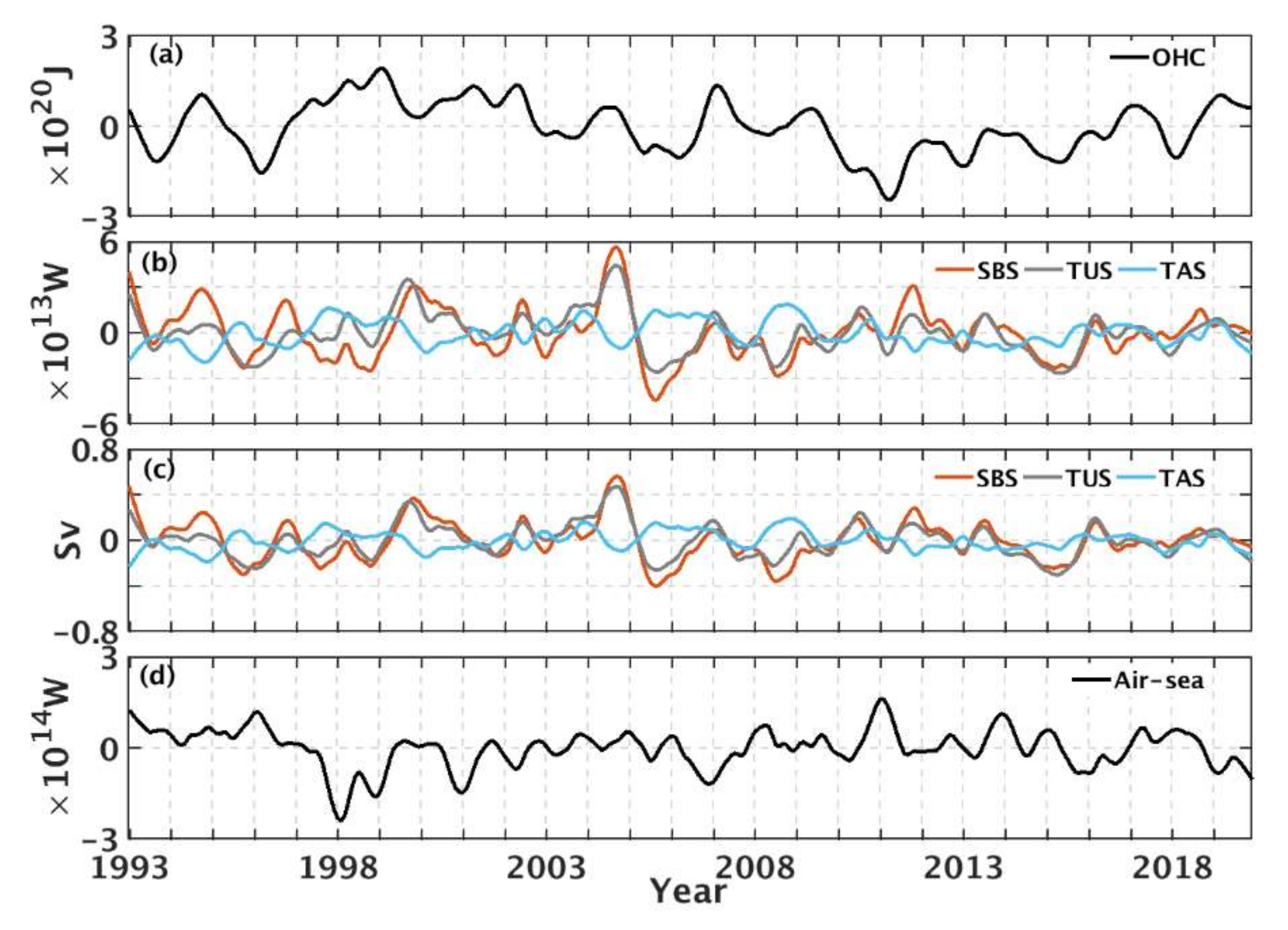
Figure 6 showed the interannual variations in the OHC, heat and volume transport across the lateral boundaries, and the sea heat flux in the BYECS shelf. From the view of the entire shelf integration, the OHC suggested a remarkable correlation with the air-sea heat flux, with a negative correlation coefficient of −0.55. The OHC was apparently larger in 1998–1999 and 2007, and smaller in 1996 and 2011 (Figure 6a), and these years corresponded to a downward (negative) and upward (positive) air-sea heat flux (Figure 6d), respectively. The interannual variation in heat transport through the SBS was greater than that across the TAS and TUS, particularly during 2004 and 2005 (Figure 6b). The years with an increase in the Kuroshio onshore intrusion and inflow from the TAS (Figure 6c) facilitated an OHC increase, although the correlation coefficients between the OHC and the two sections were low.

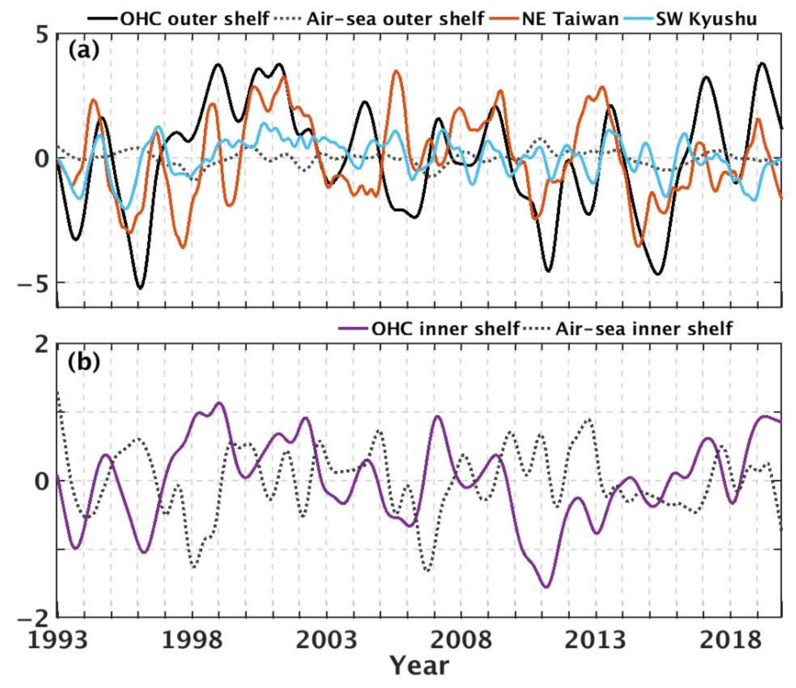
Considering the inhomogeneous OHC spatial distribution, which was approximately one order of magnitude greater in the outer shelf (between the 100 m and 200 m isobaths) compared to the inner shelf (shallower than 100 m) (Figure 3a), we inferred that the mechanisms responsible of the interannual variations of OHC in the outer and inner shelves were different. The OHC and air-sea heat flux in the outer and inner shelves were integrated between 100 m and 200 m isobaths and isobaths shallower than 100 m, respectively. Correlation analysis showed that the correlation coefficient between the OHC in the outer shelf and the heat transport across the whole SBS was not high enough (0.3), while the coefficients increased significantly when northeast Taiwan and southwest Kyushu were analyzed separately. The exchange of inflow of Kuroshio and outflow of the shelf water in the middle SBS may have an impact on the correlation analysis [24]. Figure 7a indicates that the OHC in the outer shelf showed interannual dependency on the interannual variation of heat transport through northeast Taiwan and southwest Kyushu. At a 99% confidence level, the correlation coefficient between the OHC and heat transport across northeast Taiwan was 0.47 with a lag of three months. The correlation coefficient between OHC was 0.37 for heat transport across southwest Kyushu which had no time lag. The correlation between the OHC and air-sea heat flux in the outer shelf decreased to −0.14, although the correlation over the entire shelf was greater (−0.55). Therefore, the OHC interannual variation in the outer shelf was principally modulated by the Kuroshio onshore intrusion across northeast Taiwan and southwest Kyushu.

In the inner shelf, the interannual variation of OHC was highly related to the air-sea heat flux (Figure 7b), the correlation coefficient was −0.58, and the variation of OHC lagged the variation of the air-sea heat flux by six months at a 99% confidence level. The dependency on the air-sea heat exchange increased compared to that over the entire shelf. The correlation between the OHC in the inner shelf and heat transport through the SBS was low. Therefore, the interannual OHC variations in the BYECS inner shelf were mainly associated with air-sea heat exchange. These different mechanisms of the interannual variations in the outer and inner shelves were consistent with the conclusions from the observation data and ROMS model results [13].

3.5. Long-Term Trend of OHC in the BYECS Outer Shelf

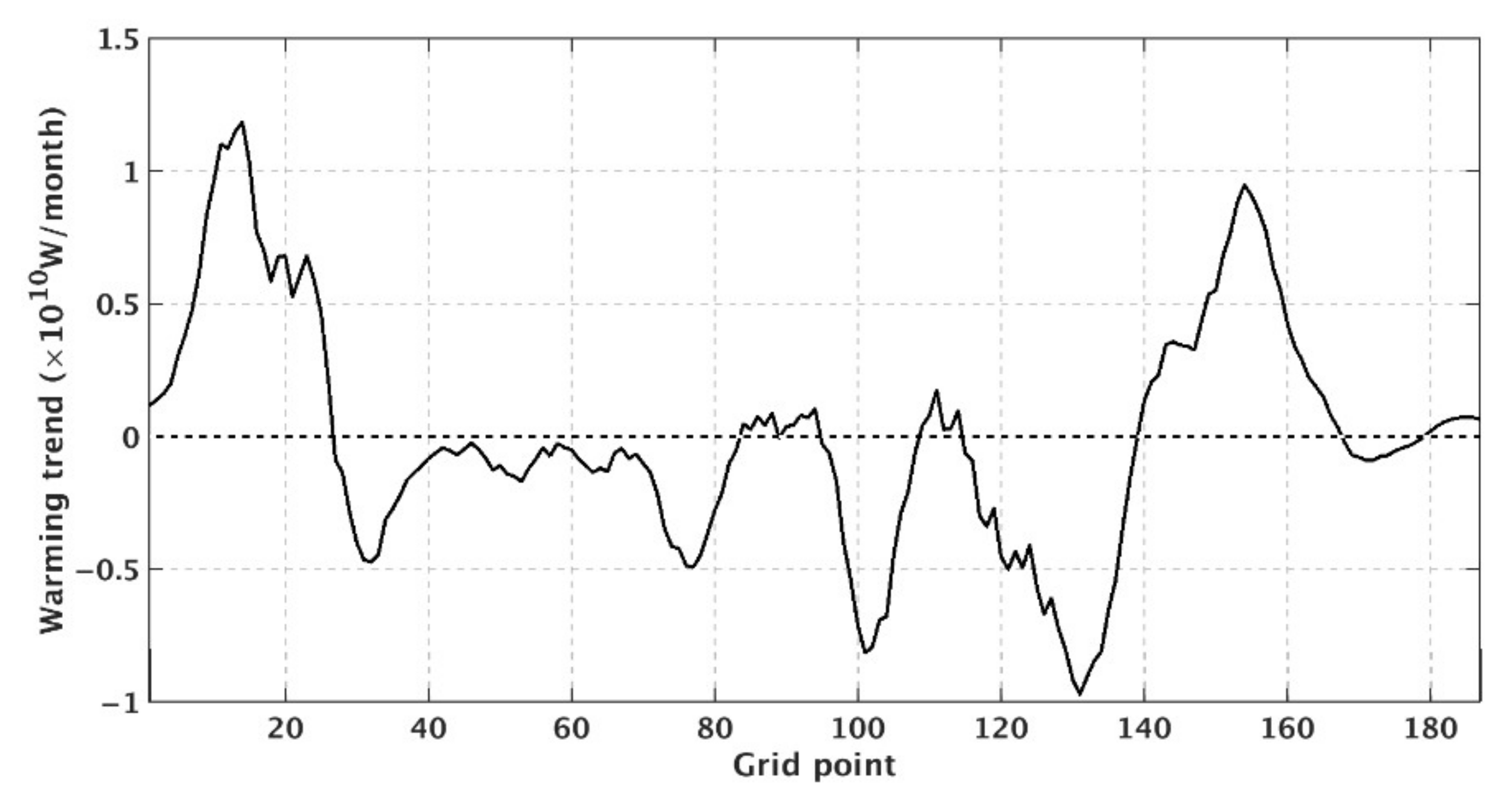
The linear trend of heat transport through the 200 m isobaths is shown in Figure 8. The onshore heat transport rates in areas northeast of Taiwan (grid points 1–27) and southwest of Kyushu (grid point 140–168) were remarkably elevated, which enabled rapid warming of the OHC in the outer shelf (Figure 3c). The trend regarding heat transport in the middle of the SBS indicated slower heat transport into the shelf, which may contribute to the OHC cooling trend in the middle SBS (Figure 3c).

The heat transport across these sections was determined by both current velocity and water temperature. To investigate their contribution to long-term variation in heat transport, we decomposed the temporal variance of heat transport into six terms [42].

The velocity (V_i) and water temperature (T_i) across one section can be described as the sum of the annual mean values ($\overline{V}$, $\overline{T}$) from 1993 to 2019 and anomalies (V’, T’). V_i and T_i are calculated as follows:

$$V_i=\overline{V}+V_i^{\prime },T_i=\overline{T}+T_i^{\prime }$$

(6)

$$\overline{V}=\frac{1}{N}{\displaystyle \sum }_{i=1}^N{V}_i,\overline{T}=\frac{1}{N}{\displaystyle \sum }_{i=1}^N{T}_i$$

(7)

where N = 324 is the number of months analyzed, and i is the time index. Then the heat flux (Q_i = V_iT_i) can be expressed as:

$$Q_i=\overline{V}\overline{T}+\overline{V}{T}_i^{\prime }+V_i^{\prime }\overline{T}+V_i^{\prime }{T}_i^{\prime }$$

(8)

Then, the annual mean heat flux (Q) is calculated as:

$$\overline{Q}=\overline{V}\overline{T}+\frac{1}{N}{\displaystyle \sum }_{i=1}^N{V}_i^{\prime }{T}_i^{\prime }$$

(9)

When defining a new term G_i = V_i’T_i’, we have:

$$\overline{G}=\frac{1}{N}{\displaystyle \sum }_{i=1}^N{V}_i^{\prime }{T}_i^{\prime }$$

(10)

Then,

$$\overline{Q}=\overline{V}\overline{T}+\overline{G}$$

(11)

The variance of heat flux (${\sigma }_Q^2$):

$${\sigma }_Q^2=\frac{1}{N}{\displaystyle \sum }_{i=1}^N(Q_i-\overline{Q}{)}^2$$

(12)

Substituting Equations (8) and (9) into Equation (12), the heat flux variance may be expressed as:

$${\sigma }_Q^2={\overline{T}}^2{\sigma }_V^2+{\overline{V}}^2{\sigma }_T^2+2\overline{T}\overline{V}{\sigma }_{TV}^2+2\overline{T}{\sigma }_{VG}^2+2\overline{V}{\sigma }_{TG}^2+{\sigma }_G^2$$

(13)

where,

$${\sigma }_V^2=\frac{1}{N}{\displaystyle \sum }_{i=1}^N(V_i-\overline{V}{)}^2,{\sigma }_T^2=\frac{1}{N}{\displaystyle \sum }_{i=1}^N(T_i-\overline{T}{)}^2$$

(14)

$${\sigma }_{TV}^2=\frac{1}{N}{\displaystyle \sum }_{i=1}^N{V}_i-\overline{V}{T}_i-\overline{T},{\sigma }_{VG}^2=\frac{1}{N}{\displaystyle \sum }_{i=1}^N(V_i-\overline{V})(G_i-\overline{G})$$

(15)

$${\sigma }_{TG}^2=\frac{1}{N}{\displaystyle \sum }_{i=1}^N{T}_i-\overline{T}{G}_i-\overline{G},{\sigma }_G^2=\frac{1}{N}{\displaystyle \sum }_{i=1}^N(G_i-\overline{G}{)}^2$$

(16)

${\overline{T}}^2{\sigma }_V^2$ denotes the mean water temperature and variance of velocity; ${\overline{V}}^2{\sigma }_T^2$ denotes the mean velocity and variance of water temperature; $2\overline{T}\overline{V}{\sigma }_{TV}^2$ denotes the mean velocity, mean water temperature, and covariance of velocity and water temperature; $2\overline{T}{\sigma }_{VG}^2$ denotes the mean water temperature and covariance of velocity; G_i; $2\overline{V}{\sigma }_{TG}^2$ denotes the mean velocity and covariance of water temperature; and G_i; ${\sigma }_G^2$ is the variance of G_i.

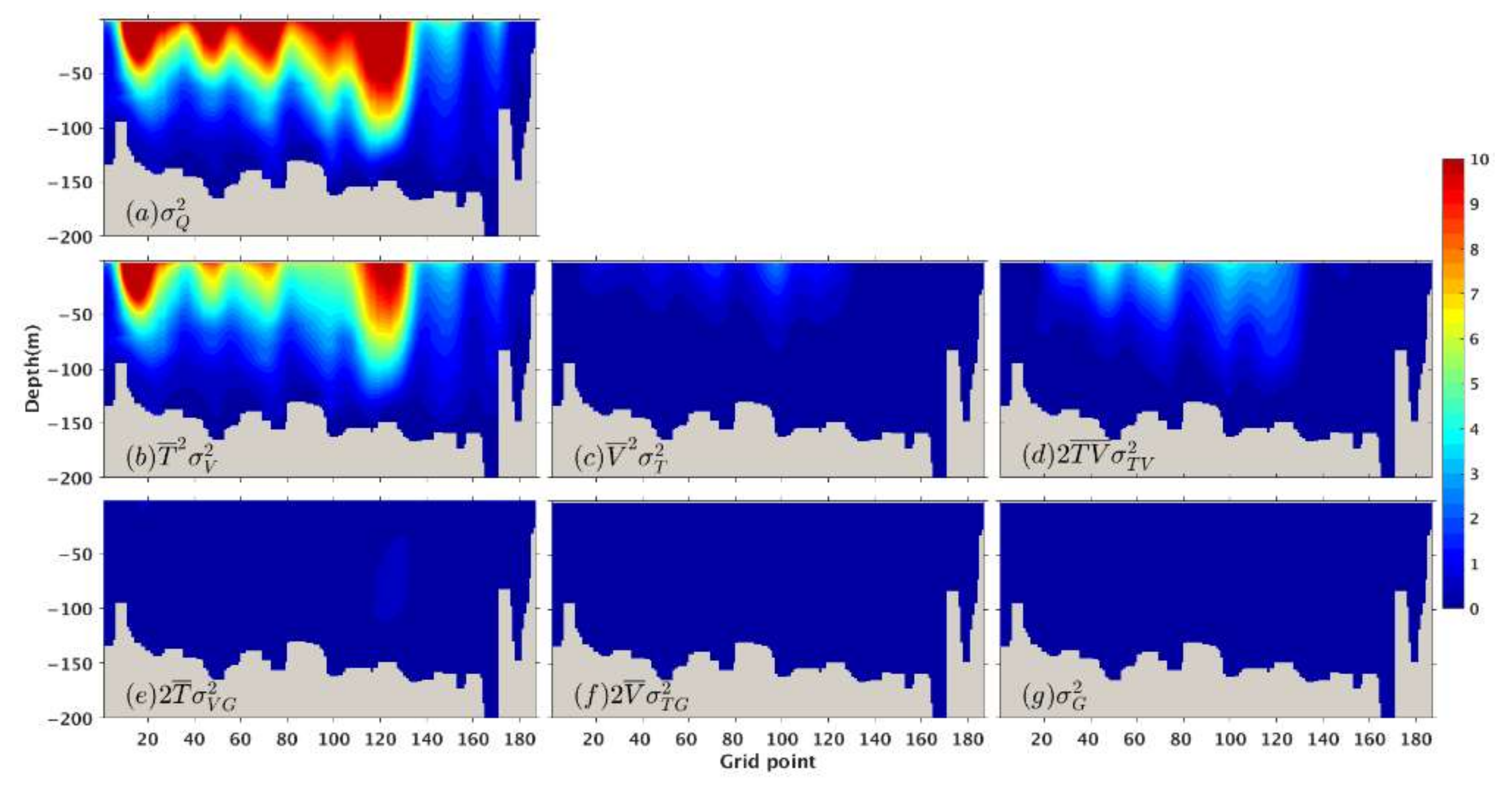
Figure 9a shows the variance of heat transport across the SBS and Figure 9b–g presented six terms on the right-hand side of Equation (13). The term of ${\overline{T}}^2{\sigma }_V^2$ accounts for the most prominent variation in heat transport (${\sigma }_Q^2$). In the northeast of Taiwan (grid ppoints 5–40), the heat transport from the Kuroshio intrusion is principally determined by the temporal variation of the current velocity. The terms of $2\overline{T}\overline{V}{\sigma }_{TV}^2$ and $2\overline{T}\overline{V}{\sigma }_{TV}^2$ also have an effect on the heat flux, although they are smaller than the term of ${\overline{T}}^2{\sigma }_V^2$.

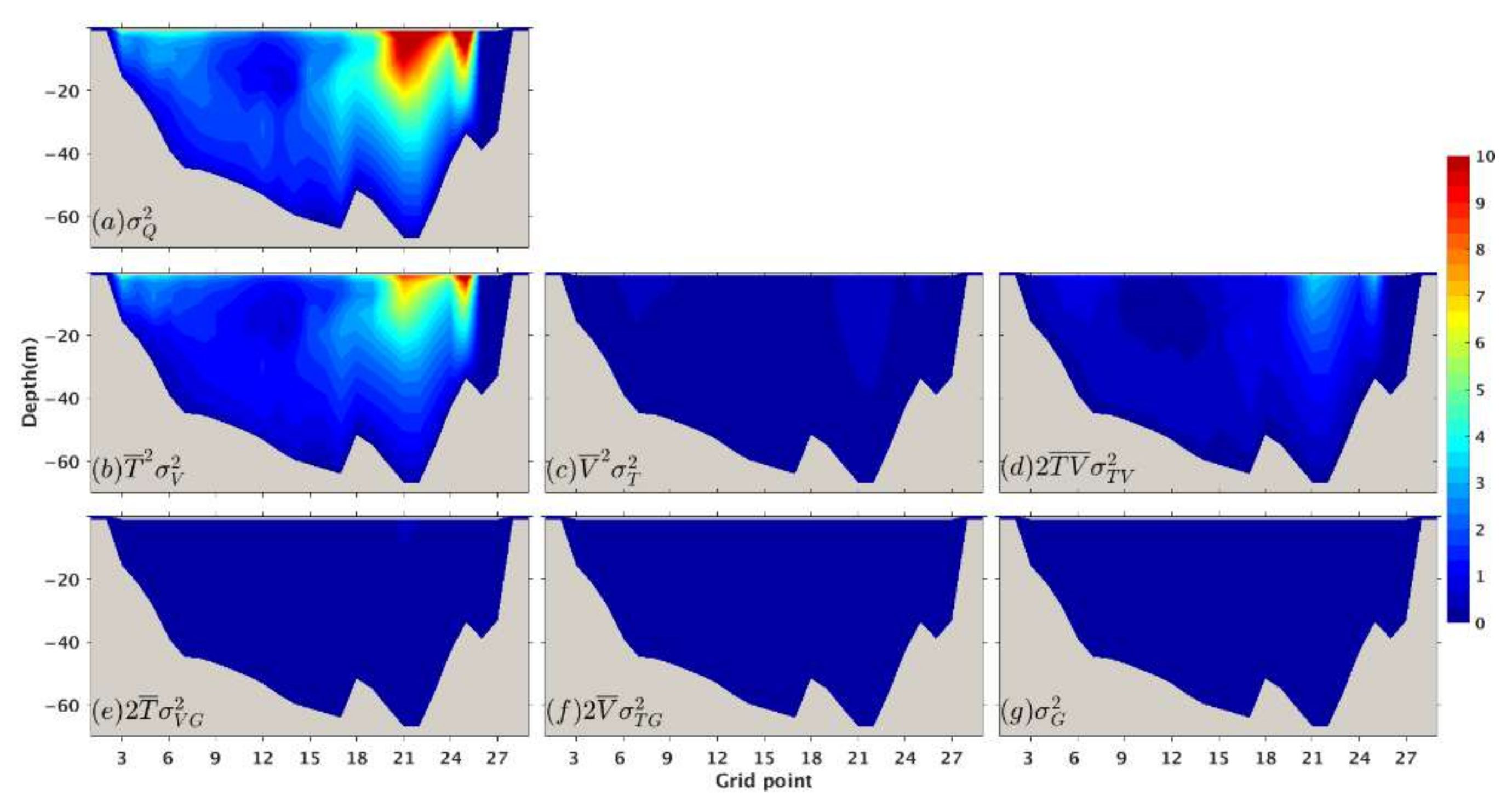
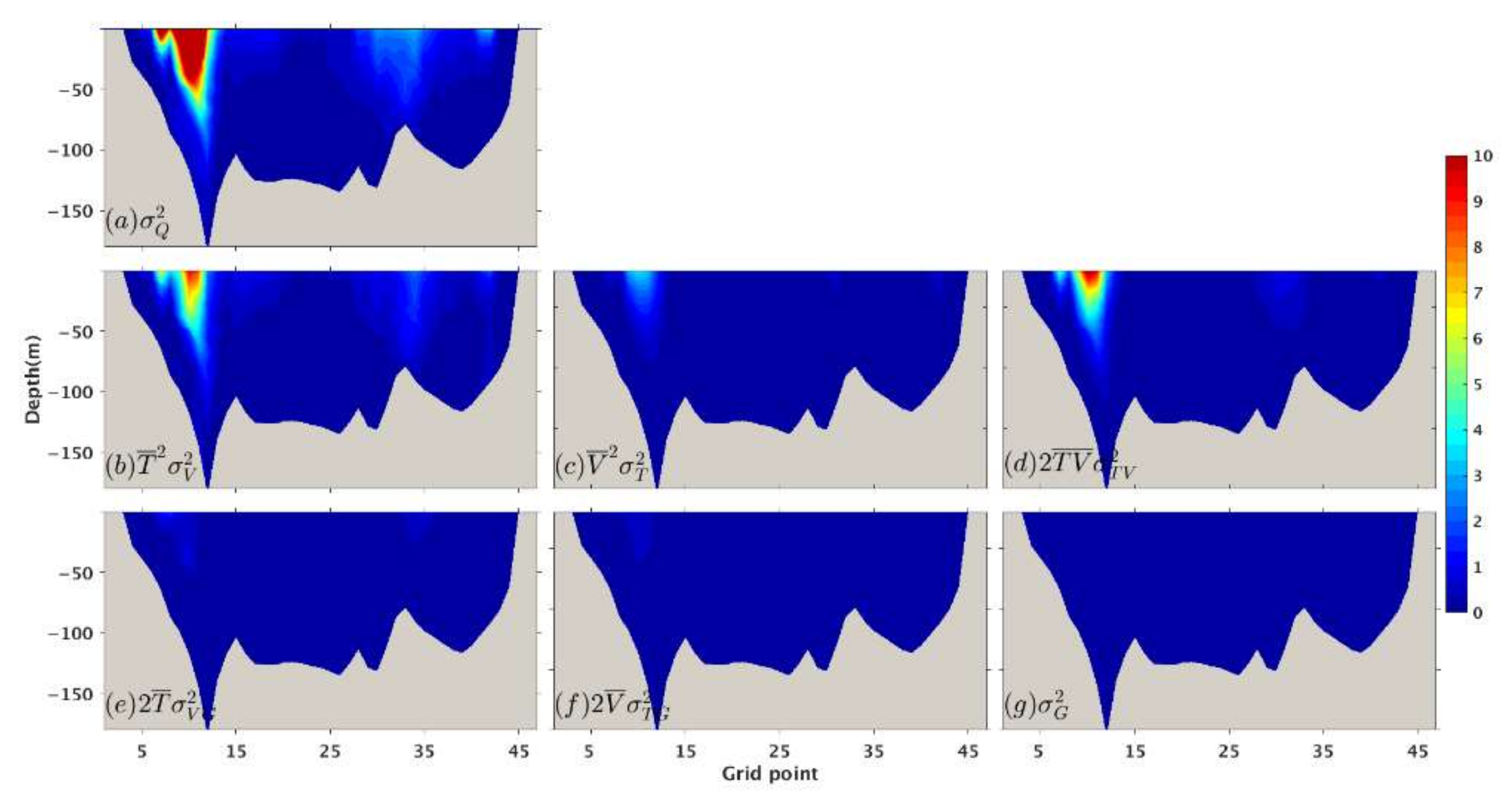
The variances of heat transport across the TAS and TUS and the corresponding six terms were in Figure 10 and Figure 11. For TAS, the variance of heat flux was large on the east side of the TAS (Figure 10a), and it was remarkable that the term of ${\overline{T}}^2{\sigma }_V^2$ (Figure 10b) was the dominant component in the variance of heat transport. The variance of heat transport through the TUS was remarkable in the west of the TUS (Figure 11a), and the term of ${\overline{T}}^2{\sigma }_V^2$ contributes most of the temporal variation of the heat flux (Figure 11b).

Analysis of the heat transport variance across the SBS, TAS, and TUS confirmed that the temporal variation in current velocity played a decisive role in the long-term trends of heat transport inflow and outflow of the lateral boundaries, and the covariance of velocity and water temperature also contributed to the temporal heat transport variation.

4. Conclusions

This study estimated the OHC for the BYECS shelf and examined its interannual variation and long-term trends using the JCOPE2M reanalysis data from 1993 to 2019. The annual mean OHC was 4.25 × 10²¹ J, with a linearly increasing warming trend of 0.13 W m⁻². The annual OHC and linear trend in the ECS are distributed inhomogeneous, and a considerable quantity of heat is stored on the outer shelf, which is one order of magnitude greater than that on the inner shelf. The warming trend was also much more rapid in the areas northeast of Taiwan and southwest of Kyushu compared to other regions, with a maximum warming rate of 0.93 W m⁻², which was approximately greater than that of the Pacific and global oceans by a factor of 4–5. However, the OHC in the middle of the 200 m isobaths showed a cooling trend. A heat budget calculation indicated that the annual mean heat transports are 1.32 × 10¹⁴, 0.87 × 10¹⁴, and −1.92 × 10¹⁴ W across the TAS, SBS, and TUS, respectively. Heat transport from the TAS contributes the greatest quantity of heat to the BYECS. The net heat gain from the lateral boundaries was 0.27 × 10¹⁴ W, which was balanced by the sea heat exchange. The net heat loss from the air-sea heat flux was particularly remarkable in areas northeast of Taiwan and southwest of Kyushu.

The interannual variation in OHC is discussed separately in the outer and inner shelves. In the outer shelf (between 100 m and 200 m isobaths), the OHC interannual variation was dependent on the Kuroshio onshore intrusion in the northeast of Taiwan and southwest of Kyushu, whereas, in the inner shelf, the interannual variation of OHC was highly related to the variation of the air-sea heat flux. The heat gain rate across the SBS was remarkably high in northeast Taiwan and southwest Kyushu, which favored rapid warming of the outer shelf. Temporal variance analysis of heat transport through the SBS demonstrated that the current velocity variation dominated the temporal variation of heat transport into the shelf. In addition, water temperature also contributed to heat transport variation.

References

- Garcia-Soto, C.; Cheng, L.; Caesar, L.; Schmidtko, S.; Jewett, E.B.; Cheripka, A.; Rigor, I.; Caballero, A.; Chiba, S.; Báez, J.C.; et al. An Overview of Ocean Climate Change Indicators: Sea Surface Temperature, Ocean Heat Content, Ocean PH, Dissolved Oxygen Concentration, Arctic Sea Ice Extent, Thickness and Volume, Sea Level and Strength of the AMOC (Atlantic Meridional Overturning Circulation). Front. Mar. Sci. 2021, 8, 642372. [Google Scholar] [CrossRef]
- Ishii, M.; Fukuda, Y.; Hirahara, S.; Yasui, S.; Suzuki, T.; Sato, K. Accuracy of Global Upper Ocean Heat Content Estimation Expected from Present Observational Data Sets. Sola 2017, 13, 163–167. [Google Scholar] [CrossRef]
- Cheng, L.; Zhu, J.; Abraham, J.; Trenberth, K.E.; Fasullo, J.T.; Zhang, B.; Yu, F.; Wan, L.; Chen, X.; Song, X. 2018 Continues Record Global Ocean Warming. Adv. Atmos. Sci. 2019, 36, 249–252. [Google Scholar] [CrossRef]
- Palmer, M.D.; Good, S.A.; Haines, K.; Rayner, N.A.; Stott, P.A. A New Perspective on Warming of the Global Oceans. Geophys. Res. Lett. 2009, 36, L20709. [Google Scholar] [CrossRef]
- Na, H.; Kim, K.-Y.; Chang, K.-I.; Park, J.J.; Kim, K.; Minobe, S. Decadal Variability of the Upper Ocean Heat Content in the East/Japan Sea and Its Possible Relationship to Northwestern Pacific Variability: Decadal Variations in the East/Japan Sea. J. Geophys. Res. 2012, 117, C02017. [Google Scholar] [CrossRef]
- Wu, L.; Cai, W.; Zhang, L.; Nakamura, H.; Timmermann, A.; Joyce, T.; McPhaden, M.J.; Alexander, M.; Qiu, B.; Visbeck, M.; et al. Enhanced Warming over the Global Subtropical Western Boundary Currents. Nat. Clim. Chang. 2012, 2, 161–166. [Google Scholar] [CrossRef]
- Huang, D.; Ni, X.; Tang, Q.; Zhu, X.; Xu, D. Spatial and Temporal Variability of Sea Surface Temperature in the Yellow Sea and East China Sea over the Past 141 Years. In Modern Climatology; Wang, S.-Y.S., Ed.; InTech: Richardson, TX, USA, 2012; ISBN 978-953-51-0095-9. [Google Scholar]
- Breitburg, D.; Levin, L.A.; Oschlies, A.; Grégoire, M.; Chavez, F.P.; Conley, D.J.; Garçon, V.; Gilbert, D.; Gutiérrez, D.; Isensee, K.; et al. Declining Oxygen in the Global Ocean and Coastal Waters. Science 2018, 359, eaam7240. [Google Scholar] [CrossRef]
- Lin, C.; Su, J.; Xu, B.; Tang, Q. Long-Term Variations of Temperature and Salinity of the Bohai Sea and Their Influence on Its Ecosystem. Prog. Oceanogr. 2001, 49, 7–19. [Google Scholar] [CrossRef]
- Yeh, S.-W.; Kim, C.-H. Recent Warming in the Yellow/East China Sea during Winter and the Associated Atmospheric Circulation. Cont. Shelf Res. 2010, 30, 1428–1434. [Google Scholar] [CrossRef]
- Tang, X.; Wang, F.; Chen, Y.; Li, M. Warming Trend in Northern East China Sea in Recent Four Decades. Chin. J. Oceanol. Limnol. 2009, 27, 185. [Google Scholar] [CrossRef]
- Bao, B.; Ren, G. Climatological Characteristics and Long-Term Change of SST over the Marginal Seas of China. Cont. Shelf Res. 2014, 77, 96–106. [Google Scholar] [CrossRef]
- Sasaki, Y.N.; Umeda, C. Rapid Warming of Sea Surface Temperature along the Kuroshio and the China Coast in the East China Sea during the Twentieth Century. J. Clim. 2021, 34, 4803–4815. [Google Scholar] [CrossRef]
- Zhang, L.; Wu, L.; Lin, X.; Wu, D. Modes and Mechanisms of Sea Surface Temperature Low-Frequency Variations over the Coastal China Seas. J. Geophys. Res. Oceans 2010, 115, C08031. [Google Scholar] [CrossRef]
- Cai, R.; Tan, H.; Kontoyiannis, H. Robust Surface Warming in Offshore China Seas and Its Relationship to the East Asian Monsoon Wind Field and Ocean Forcing on Interdecadal Time Scales. J. Clim. 2017, 30, 8987–9005. [Google Scholar] [CrossRef]
- Wijffels, S.; Roemmich, D.; Monselesan, D.; Church, J.; Gilson, J. Ocean Temperatures Chronicle the Ongoing Warming of Earth. Nat. Clim. Chang. 2016, 6, 116–118. [Google Scholar] [CrossRef]
- Trenberth, K.E.; Cheng, L.; Jacobs, P.; Zhang, Y.; Fasullo, J. Hurricane Harvey Links to Ocean Heat Content and Climate Change Adaptation. Earth’s Future 2018, 6, 730–744. [Google Scholar] [CrossRef]
- Tian, D.; Su, J.; Zhou, F.; Mayer, B.; Sein, D.; Zhang, H.; Huang, D.; Pohlmann, T. Heat Budget Responses of the Eastern China Seas to Global Warming in a Coupled Atmosphere–ocean Model. Clim. Res. 2019, 79, 109–126. [Google Scholar] [CrossRef]
- Harley, C.D.G.; Randall Hughes, A.; Hultgren, K.M.; Miner, B.G.; Sorte, C.J.B.; Thornber, C.S.; Rodriguez, L.F.; Tomanek, L.; Williams, S.L. The Impacts of Climate Change in Coastal Marine Systems. Ecol. Lett. 2006, 9, 228–241. [Google Scholar] [CrossRef]
- Gilbert, D.; Rabalais, N.N.; Díaz, R.J.; Zhang, J. Evidence for Greater Oxygen Decline Rates in the Coastal Ocean Than in the Open Ocean. Biogeosciences 2010, 7, 2283–2296. [Google Scholar] [CrossRef]
- Guo, X.; Miyazawa, Y.; Yamagata, T. The Kuroshio Onshore Intrusion along the Shelf Break of the East China Sea: The Origin of the Tsushima Warm Current. J. Phys. Oceanogr. 2006, 36, 2205–2231. [Google Scholar] [CrossRef]
- Liu, C.; Wang, F.; Chen, X.; von Storch, J.-S. Interannual Variability of the Kuroshio Onshore Intrusion along the East China Sea Shelf Break: Effect of the Kuroshio Volume Transport. J. Geophys. Res. Oceans 2014, 119, 6190–6209. [Google Scholar] [CrossRef]
- Song, J.; Xue, H.; Bao, X.; Wu, D.; Chai, F.; Shi, L.; Yao, Z.; Wang, Y.; Nan, F.; Wan, K. A Spectral Mixture Model Analysis of the Kuroshio Variability and the Water Exchange between the Kuroshio and the East China Sea. Chin. J. Oceanol. Limnol. 2011, 29, 446–459. [Google Scholar] [CrossRef]
- Zhang, J.; Guo, X.; Zhao, L.; Miyazawa, Y.; Sun, Q. Water Exchange across Isobaths over the Continental Shelf of the East China Sea. J. Phys. Oceanogr. 2017, 47, 1043–1060. [Google Scholar] [CrossRef]
- Liu, N.; Eden, C.; Dietze, H.; Wu, D.; Lin, X. Model-Based Estimate of the Heat Budget in the East China Sea. J. Geophys. Res. Oceans 2010, 115, C08026. [Google Scholar] [CrossRef]
- Zhou, F.; Xue, H.; Huang, D.; Xuan, J.; Ni, X.; Xiu, P.; Hao, Q. Cross-Shelf Exchange in the Shelf of the East China Sea. J. Geophys. Res. Oceans 2015, 120, 1545–1572. [Google Scholar] [CrossRef]
- Zhang, Q.; Hou, Y.; Yan, T. Inter-Annual and Inter-Decadal Variability of Kuroshio Heat Transport in the East China Sea. Int. J. Climatol. 2012, 32, 481–488. [Google Scholar] [CrossRef]
- Mellor, G.L.; Häkkinen, S.M.; Ezer, T.; Patchen, R.C. A Generalization of a Sigma Coordinate Ocean Model and an Intercomparison of Model Vertical Grids. In Ocean Forecasting: Conceptual Basis and Applications; Pinardi, N., Woods, J., Eds.; Springer: Berlin/Heidelberg, Germany, 2002; pp. 55–72. ISBN 978-3-662-22648-3. [Google Scholar]
- Uehara, K.; Saito, Y.; Hori, K. Paleotidal Regime in the Changjiang (Yangtze) Estuary, the East China Sea, and the Yellow Sea at 6 Ka and 10 Ka Estimated from a Numerical Model. Mar. Geol. 2002, 183, 179–192. [Google Scholar] [CrossRef]
- Kalnay, E.; Kanamitsu, M.; Kistler, R.; Collins, W.; Deaven, D.; Gandin, L.; Iredell, M.; Saha, S.; White, G.; Woollen, J.; et al. The NCEP/NCAR 40-Year Reanalysis Project. Bull. Am. Meteorol. Soc. 1996, 77, 437–472. [Google Scholar] [CrossRef]
- Kagimoto, T.; Miyazawa, Y.; Guo, X.; Kawajiri, H. High Resolution Kuroshio Forecast System: Description and Its Applications. In High Resolution Numerical Modelling of the Atmosphere and Ocean; Hamilton, K., Ohfuchi, W., Eds.; Springer: New York, NY, USA, 2008; pp. 209–239. ISBN 978-0-387-49791-4. [Google Scholar]
- Guo, X.; Hukuda, H.; Miyazawa, Y.; Yamagata, T. A Triply Nested Ocean Model for Simulating the Kuroshio—Roles of Horizontal Resolution on JEBAR. J. Phys. Oceanogr. 2003, 33, 146–169. [Google Scholar] [CrossRef]
- Miyazawa, Y.; Zhang, R.; Guo, X.; Tamura, H.; Ambe, D.; Lee, J.-S.; Okuno, A.; Yoshinari, H.; Setou, T.; Komatsu, K. Water Mass Variability in the Western North Pacific Detected in a 15-Year Eddy Resolving Ocean Reanalysis. J. Oceanogr. 2009, 65, 737–756. [Google Scholar] [CrossRef]
- Miyazawa, Y.; Varlamov, S.M.; Miyama, T.; Guo, X.; Hihara, T.; Kiyomatsu, K.; Kachi, M.; Kurihara, Y.; Murakami, H. Assimilation of High-Resolution Sea Surface Temperature Data into an Operational Nowcast/Forecast System around Japan Using a Multi-Scale Three-Dimensional Variational Scheme. Ocean Dyn. 2017, 67, 713–728. [Google Scholar] [CrossRef]
- Isobe, A. Recent Advances in Ocean-Circulation Research on the Yellow Sea and East China Sea Shelves. J. Oceanogr. 2008, 64, 569–584. [Google Scholar] [CrossRef]
- Teague, W.J.; Jacobs, G.A.; Perkins, H.T.; Book, J.W. Low-Frequency Current Observations in the Korea/Tsushima Strait. J. Phys. Oceanogr. 2002, 32, 21. [Google Scholar]
- Takikawa, T.; Yoon, J.-H.; Cho, K.-D. The Tsushima Warm Current through Tsushima Straits Estimated from Ferryboat ADCP Data. J. Phys. Oceanogr. 2005, 35, 1154–1168. [Google Scholar] [CrossRef]
- Fukudome, K.-I.; Yoon, J.-H.; Ostrovskii, A.; Takikawa, T.; Han, I.-S. Seasonal Volume Transport Variation in the Tsushima Warm Current through the Tsushima Straits from 10 Years of ADCP Observations. J. Oceanogr. 2010, 66, 539–551. [Google Scholar] [CrossRef]
- Guihua, W.; Rongfeng, L.; Changxiang, Y. Advances in Studying Oceanic Circulation from Hydrographic Data with Applications in the South China Sea. Adv. Atmos. Sci. 2003, 20, 914–920. [Google Scholar] [CrossRef]
- World Ocean Atlas 2018, Volume 1: Temperature. Available online: https://www.researchgate.net/publication/335057554_World_Ocean_Atlas_2018_Volume_1_Temperature (accessed on 13 July 2022).
- Seo, G.-H.; Cho, Y.-K.; Choi, B.-J. Variations of Heat Transport in the Northwestern Pacific Marginal Seas Inferred from High-Resolution Reanalysis. Prog. Oceanogr. 2014, 121, 98–108. [Google Scholar] [CrossRef]
- Guo, X.; Zhu, X.-H.; Wu, Q.-S.; Huang, D. The Kuroshio Nutrient Stream and Its Temporal Variation in the East China Sea. J. Geophys. Res. Oceans 2012, 117, C01026. [Google Scholar] [CrossRef] [Green Version]
Figure 1.
Annual-mean sea surface current distribution in the Bohai Sea, Yellow Sea, and East China Sea (BYECS, black arrows). The study region (BYECS) is closed with three lines indicating the Taiwan Strait (TAS), shelf break section (SBS, 200-m isobath), and Tsushima Strait (TUS). Between each set of adjacent red dots on the black lines, there are 20 grid points. The grid points are counted from south to north. Arrows across these black lines represent heat (volume) transport across the sections measured in ×1014 W (Sv, ×106 m3 s−1). Gray contour lines represent the 100-m isobaths, the Kuroshio enters the East China Sea from the East Taiwan Channel (ETC).
Figure 2.
Climatology of water temperature. (a,c) are the annual-mean (2005–2017) temperature distributions at the sea surface and 124° E from the JCOPE2M reanalysis data, respectively. (b,d) are plots of the same, but from the WOA2018 dataset. The red line in (a) denotes the section at 124° E.
Figure 3.
(a) Annual mean (×109 J m−2), (b) standard deviation (×108 J m−2), and (c) linear increasing trend (W m−2) of the OHC in the BYECS over the 1993–2019 period from the JCOPE2M reanalysis data.
Figure 4.
(a) Vertical distribution of the annual-mean heat transport across the SBS. (b,c) are identical plots for the TAS and TUS, respectively. The locations of these three sections are provided in Figure 1.
Figure 5.
(a) Annual mean (W m−2), (b) standard deviation (W m−2), and (c) linear trend (W m−2 month−1) for the air-sea heat flux in the BYECS during the 1993–2019 period from the JCOPE2M reanalysis data.
Figure 6.
(a) Interannual OHC variation integrated over the BYECS from 1993 to 2019. (b) Interannual variation of heat transport across the SBS (orange solid line), TUS (gray solid line), and TAS (blue solid line). (c) Interannual variation of volume transport across the SBS (orange solid line), TUS (gray solid line), and TAS (blue solid line). (d) Interannual variation of air-sea heat flux integrated over the BYECS.
Figure 7.
(a) Interannual OHC variations (×1019 J, black solid line) and air-sea heat flux (×1013 W, gray dash line) integrated over the outer shelf of the BYECS, heat transport (×1014 W) across the SBS northeast of Taiwan (orange solid line) and that located southwest of Kyushu (blue solid line). (b) Interannual OHC variations (×1020 J, purple solid line) and air-sea heat flux (×1013 W, gray dash line) integrated over the inner shelf of the BYECS.
Figure 8.
The trend of vertical-integrated heat transport at each point along the SBS.
Figure 9.
(a) denotes the total variance in heat transport across the SBS. (b–g) represent the six terms decomposed using Equation (13).
Figure 10.
(a) denotes the total variance in heat transport across the TAS. (b–g) represent the six terms decomposed using Equation (13).
Figure 11.
(a) denotes the total variance in heat transport across the TUS. (b–g) represent the six terms decomposed using Equation (13).