Research on Temporal and Spatial Differentiation and Impact Paths of Agricultural Grey Water Footprints in the Yellow River Basin

Abstract

The scientific evaluation of water pollution in the Yellow River Basin was directly related to the sustainable utilization of water resources and the green development of the agricultural economy in this region. In this study, we focused on the planting industry, and measured the agricultural grey water footprint of 73 prefecture-level cities in the Yellow River Basin from 2000 to 2019. We used spatial autocorrelation analysis to reveal temporal and spatial differentiation characteristics, and we used the path analysis method to study the factors influencing the temporal evolution and spatial distribution. Taking 2015 as the study period, the agricultural grey water footprint showed a trend of first rising and then falling. The values and growth rates of the agricultural grey water footprint in different regions were quite different. According to the natural breakpoint method, the agricultural grey water footprints were divided into low, middle, high, and very high groups. There were obvious spatial differences in the agricultural grey water footprints, and these differences gradually decreased. Generally, the H–L and the L–L types were dominant. From 2000 to 2019, most prefecture-level cities maintained the same transition changes as those in the neighboring regions. Crop yield, economic scale, population scale, urban and rural structure, and technological innovation were found to be the key elements of spatiotemporal variation in the agricultural grey water footprint.

1. Introduction

In 2022, Central Document No. 1 clearly proposes to “promote the green development in agriculture and rural areas, strengthen comprehensive efforts to control pollution from non-point agricultural sources, further reduce agricultural investment, strengthen the resource utilization of livestock and poultry manure, promote the scientific use and recycling of agricultural film, and develop agricultural evaluation of green development”, which is a very important theoretical proposition. The Yellow River Basin is an important ecological barrier and food base in China, and it is also an important ecological barrier and economic zone [1]. However, it has a fragile ecological background, a high resource and environment load, insufficient economic development and low development quality, and it is also the area with the highest agricultural water pressure in China [2]. In September 2019, the Chinese government highlighted “ecological protection and high-quality development of the Yellow River Basin” as a major national strategy. In 2020, the grain output in the nine provinces and autonomous regions along the Yellow River was about 239 million tons, an increase of 2.14% over the previous year, accounting for about 35.6% of the national total. The GDP of the primary industry was about CNY 2.34 trillion, an increase of 11.96% over the previous year, accounting for about 30.1% of the country. However, prioritizing food security has led to the externalization of the environmental cost of water resources in the Yellow River Basin, coupled with the inherent spatial–temporal dislocation of water resources. This has further aggravated the water resources shortage and water environment pollution, and severely restricted the green development of agriculture and rural areas in the Yellow River Basin [3,4]. According to the results of China’s second survey of pollution sources, in 2017, chemical oxygen demand (COD), total nitrogen (TN), and total phosphorus (TP) emissions from agricultural sources and rural household sources accounted for 80.6%, 53.0%, and 74.1% of the total pollutants emissions in the Yellow River Basin, respectively. This was higher than the national averages of 85.90%, 10.21%, and 1.36%. Agricultural non-point source pollution is relatively serious [5]. Therefore, under the condition of ensuring the sustainable utilization of water resources and the green development of agriculture, it is of great significance to improve agricultural water quality and efficiency, which is firstly based on the scientific evaluation of the agricultural water environment.

As a method by which to measure the impact of human activities on the water resources systems, the water footprint comprehensively investigates the direct and indirect water use, water consumption, and pollution of consumers or producers. This mainly includes the blue, green, and grey water footprint, which has become a global research hotspot [6]. Among these, the grey water footprint refers to the amount of freshwater resources required to assimilate the pollutant loads discharged by the absorption products, based on the natural background concentration and the existing water environmental quality standards [7]. This method fully reflects the interaction between human economic activities and the water environment system, which is helpful for comprehensively and scientifically evaluating water pollution and achieving sustainable water use and green development [8]. Combining existing research, firstly, the grey water footprint measurement mainly focuses on the selection of key pollutants. Wickramasinghe et al. developed calibrated models and predicted the grey water footprint of eight pollutants [9]. Hong et al. selected nitrogen fertilizer as an agricultural pollution source and calculated the agricultural grey water footprint in the North China Plain from 2000 to 2016 [10]. Muratoglu evaluated the grey water footprint of 81 provinces and 25 watersheds in Turkey, using the tier-1 method and the high-resolution leachate runoff fraction [11]. Wu et al. calculated the agricultural grey water footprint under the inter-field test modes of conventional diffuse irrigation (CDI) and water-saving irrigation (WSI), by tracking the source of evapotranspiration and the migration process of various nitrogen and phosphorus pollutants [12]. Feng quantified China’s grey water footprint from 2003 to 2018 based on four pollutants: chemical oxygen demand (COD), ammonia nitrogen (NH3-N), total nitrogen (TN) and total phosphorus (TP) [13]. Most of the agricultural grey water footprint involved in the above studies were focused on the pollution of the water environment caused by the excessive application of nitrogen fertilizer, and less consideration was given to the grey water footprint caused by compound fertilizer abuse. However, nitrogen was the main element in nitrogen fertilizer, for example, the nitrogen content of amide nitrogen was high, which was 46.7%. Not all nitrogen fertilizers had 100% nitrogen content. In addition, compound fertilizer also contained 30% nitrogen element, which would also cause pollution to underground water. Ignoring nitrogen element pollution caused by compound fertilizer application would lead to bias in the research results. Secondly, regarding the temporal–spatial characteristics of the grey water footprint, Xie et al. measured and analyzed the green, blue, and grey water footprints of pig feeding and pork production in China from 2004 to 2013 and their spatial and temporal evolution patterns. They concluded that, over time, the regions with higher grey water footprints generated by pig rearing began to shift southward [14]. Lin et al. analyzed the temporal and spatial distribution characteristics of the grey water footprint and the change trend of the gravity center in 31 provinces (cities and districts) of China during 1998–2016. This was on the basis of revealing the spatial evolution characteristics of the grey water footprint in China, as well as at the provincial level during 2003–2015 [15]. Li et al. adopted the ESDA (Exploratory Spatial Data Analysis) method to analyze the temporal and spatial evolution of blue water footprint and grey water footprint in the Haihe River Basin [16]. Ma et al. used the water footprint method to investigate the dynamic evolution of agricultural water consumption from 2005 to 2015 in Zhangjiakou, an extremely water-scarce city which was divided into six ecological zones (I, II, III, IV, V, and VI) [17]. The above studies provide a new perspective for the scientific evaluation of regional water environmental pollution [18,19,20]. However, the above studies only involved the grey water footprint at the national and provincial level, and there were few scholars in the perspective of river basin, on the scale of the space of the city level difference of grey water footprint system analysis and in-depth exploration, however, the river basin as a special geographical unit, the space had features such as integrity, extents and differences, grey water footprint on the basin geographical unit of space law how to present, was in line with the basin, which was a special geographical unit features, this kind of research had important guiding significance for the sustainable development of water resources environment in the basin. Finally, regarding factors affecting water footprint, He and Xiang calculated the grey water footprint of pollutants diluted by the agricultural, industrial, and livestock sectors in Hunan Province from 2001 to 2015, and analyzed the influencing factors using the extended STIRPAT (Stochastic Impacts by Regression on Population, Affluence and Technology) model. The urbanization level, proportion of tertiary industry, proportion of secondary industry, per capita GDP, intensity of grey water footprint, and foreign direct investment were the main influencing factors of the grey water footprint [21]. Based on the MRIO model and combined with an improved grey water footprint calculation method, Li et al. studied the impact of regional trade on China’s grey water footprint, and found that coexisting compounds had a greater impact on the grey water footprint, while the effect of inter-regional trade on improving China’s grey water footprint was not significant [22]. Li et al. calculated the water footprint generated by rice planting in 30 provinces (cities and districts) in China from 1996 to 2015 and determined its spatio-temporal influencing factors, finding that average temperature (ATE), irrigation water coefficient (IWC) and fertilizer application amount in a sown area (FER) all positively affected the water footprint in time and space [23]. Wang et al. analyzed the factors influencing the agricultural water footprint across desert regions of northern China, from 2003 to 2017, and found that potential evapotranspiration was the main influencing factor, which explained 20.4% of the variation in the agricultural water footprint [24]. Based on the quantification of the blue water footprint and the green water footprint of major food crop production in 11 cities of Shanxi Province from 2005 to 2014, Feng et al. analyzed the spatiotemporal variation and climate influencing factors in combination with agricultural and climate data and found that sunshine, temperature, and rainfall, among various climate factors, were the main driving factors of the crop production water footprint [25]. Cai et al. evaluated Chinese agricultural water footprints from 2000 to 2017 and analyzed the influencing factors, and found that GDP per capita, total investment in fixed assets, the income level of rural residents, the proportion of food grown, spray and drip irrigation technology, low-pressure pipe irrigation technology and seepage control irrigation technology had significant positive impacts on the agricultural water footprint. In contrast, the proportion of secondary and tertiary industries, social retail consumption, urbanization, technology expenditure, and the effective irrigation area proportion had a significant inhibitory effect [26]. Existing studies attach importance to the elaboration of econometric models, but the analysis of the action mechanism of influencing factors of grey water footprint is insufficient, and the persuasiveness needs to be strengthened. The above studies only conduct overall regression analysis based on all research samples to explore the main influencing factors, ignoring the heterogeneity of influencing factors in different regions, only discuss the various direct influencing factors of the water footprint; however, the influencing factors of the water footprint are various, including, but not limited to, meteorological factors, and agricultural production inputs, such as macro policies; additionally, the mixed and complex dynamic relationships between influencing factors have indirect effects on the water footprint. Therefore, ignoring indirect effects may lead to bias in research results. In order to overcome the defects in the above studies, this study proposes the following innovations: Firstly, when calculating the agricultural grey water footprints, the existing studies focus on the pollution of water environments caused by excessive application of chemical fertilizers (mainly nitrogen fertilizers) in the planting industry, whereas this study also considers the agricultural grey water footprint caused by other kinds of chemical fertilizers (nitrogen fertilizers and compound fertilizers), and 46% of nitrogen fertilizer content and 30% of compound fertilizer content are considered as nitrogen pollution. Secondly, most of the existing studies on the temporal and spatial characteristics of the grey water footprint only involve the provincial level, but this study comprehensively analyzes the temporal and spatial characteristics of the grey water footprint of the Yellow River Basin at the municipal level. Finally, as for studies regarding the influencing factors of water footprints, the existing studies only discuss the direct effects of various influencing factors on the water footprint, whereas we study the indirect effects of various influencing factors on the water footprint on this basis.

The marginal contribution of this paper was mainly reflected in three aspects: First, the calculation idea of grey water footprint was improved. This study not only considered the pollution of the water environment caused by excessive application of chemical fertilizers (mainly nitrogen fertilizer), but also took into account the influence of other kinds of fertilizers (nitrogen fertilizer and compound fertilizer) on the agricultural grey water footprint, which was the inheritance and expansion of existing studies. Second, for the study of the grey water footprint, this paper further considered the influence of spatial interaction, that is, to explore the interaction between regions and expand the application of spatial econometric model in this field. Third, although there have been studies on influencing factors of the grey water footprint in the academic community, the Tobit model was mainly used to analyze the impact of various indicators. This study comprehensively discusses the direct and indirect impacts of various influencing factors on the water footprint, which made up for the blind spot of empirical analysis in this field. Based on this, we focused on the planting industry, and measured the agricultural grey water footprint of 73 prefecture-level cities in the Yellow River Basin from 2000 to 2019. We used spatial autocorrelation analysis to reveal temporal and spatial differentiation characteristics, and used the path analysis method to study the factors influencing the temporal evolution and spatial distribution. This article is arranged as follows: the second part is the research methods and data sources; the third part presents the empirical analysis, including calculating the agricultural grey water footprints of 73 prefecture-level cities in the Yellow River Basin from 2000 to 2019 (using the spatial autocorrelation analysis to reveal the spatial and temporal differentiation characteristics of the agricultural grey water footprint), using the path analysis to study the influencing factors of the temporal evolution and spatial distribution of the agricultural grey water footprint; and the fourth part discusses conclusions and recommendations.

2. Research Methods and Data Sources

2.1. Research Methods

2.1.1. Agricultural Grey Water Footprint

In this study, the agricultural grey water footprint (AWF_grey) only refers to the grey water footprint of the planting industry [27,28].

Regarding crop growth, a large number of chemical fertilizers and pesticides are applied in order to reduce plant diseases and insect pests of crops and soil fertility. Most of these enter the water environment at a fixed proportion (leaching rate) under the action of the precipitation or irrigation water, causing surface runoff and underground water pollution [29]. According to the common model of the Water Footprint Assessment Manual, the grey water footprint from the planting industry can be calculated based on the leaching of nitrogen into water caused by fertilizer application (including nitrogen fertilizers and compound fertilizers) [7,30,31]. In this study, we only considered the grey water footprint of nitrogen produced by nitrogen fertilizers and compound fertilizers in the calculation [32,33,34]. The specific calculation formula is as follows [35]:

$$W{F}_{grey,plant}\left(\mathrm{TN}\right)=\frac{\alpha \times \left(APP{l}_n\times C_n+APP{l}_c\times C_c\right)}{C_{max}-C_{nat}}$$

(1)

In Equation (1), $W{F}_{grey,plant}\left(\mathrm{TN}\right)$ (m³) is the grey water footprint of the planting industry and α (%) represents the leaching rate; 7% of nitrogen was selected as the leaching rate in this study according to previous studies [32,36]. APPl is defined the abbreviation of the word “Application”. $APP{l}_n$ (kg) and $APP{l}_c$ (kg) represent the annual yield of nitrogen fertilizer and compound fertilizer, respectively [35]. $C_n$ and $C_c$ represent a nitrogen content of 46% and 30% in nitrogen fertilizer and compound fertilizer, respectively [35]. $C_{max}$ (kg/m³) represents the water quality standard concentration of the pollutant N element in chemical fertilizers required by Grade III of the Environmental Quality Standards for Surface Water in China (GB3838-2002), set at 0.001 kg/m³ [14]. $C_{nat}$ (kg/m³) represents the natural background concentration of the pollutants N element in chemical fertilizers in the receiving water, which is usually defaulted to 0 kg/ m³ [37,38].

2.1.2. Spatial Autocorrelation Analysis Method

Spatial autocorrelation is usually used to analyze the correlation level between the attribute eigenvalue of a unit in a certain region of space and the same attribute eigenvalue of the unit in its adjacent region, which can be divided into global and local spatial autocorrelation [39,40]. Global spatial autocorrelation mainly analyzes whether regions have spatial relevance on the whole level. Local spatial autocorrelation mainly studies whether there is local spatial aggregation with high or low values in specific regions, and specific indexes under the condition of regional autocorrelation as a whole [41].

(1)

Global spatial autocorrelation (global Moran’s I)

Global spatial autocorrelation can be used to analyze whether the spatial distribution of a certain attribute characteristic value of a research object is correlated in the overall research area, and to then judge whether such a phenomenon exists aggregated in space [42]. The global Moran index is a commonly used spatial autocorrelation measure, and its definition is as follows [43,44]:

$${\mathrm{Moran}}^{’}\mathrm{s}I=\frac{{{\displaystyle \sum }}_{i=1}^n{{\displaystyle \sum }}_{j\ne i}^n{W}_{ij}{z}_i{z}_j}{{\sigma }^2{{\displaystyle \sum }}_{i=1}^n{{\displaystyle \sum }}_{j\ne i}^n{W}_{ij}}$$

(2)

$$=\frac{n{{\displaystyle \sum }}_{i=1}^n{{\displaystyle \sum }}_{j\ne i}^n{W}_{ij}\left(x_i-\overline{x}\right)\left(x_j-\overline{x}\right)}{{{\displaystyle \sum }}_{i=1}^n{{\displaystyle \sum }}_{j\ne i}^n{W}_{ij}{{\displaystyle \sum }}_{i=1}^n{\left(x_i-\overline{x}\right)}^2}$$

(3)

In Equations (2) and (3), n is the number of regions in space; $x_i$ is the $AW{F}_{grey}$ of region i; $x_j$ is the $AW{F}_{grey}$ of region j; $z_i$ is the standard transformation of $x_i$ $(z_i=\frac{\left(x_i-\overline{x}\right)}{\sigma })$; $z_j$ is the standard transformation of $x_j$ ($z_j=\frac{\left(x_j-\overline{x}\right)}{\sigma }$; $\overline{x}=\frac{1}{n}{\displaystyle \sum }_{i=1}^n{x}_i$) [43]; and $W_{ij}$ is a binary adjacency space weight matrix, representing the adjacency relationship of space objects [44]. When region $i$ is adjacent to region $j$, $W_{ij}$ = 1; otherwise, $W_{ij}$ = 0, ${\sigma }^2=\frac{1}{n}{\displaystyle \sum }_{i=1}^n{\left(x_i-\overline{x}\right)}^2$ [45]. The value range of ${\mathrm{Moran}}^{’}\mathrm{s}I$ statistic is between −1 and 1. When I is within [0, 1], it indicates that there is spatial positive correlation. The closer the value is to 1, the higher the spatial correlation degree is. When I is within [−1, 0], it indicates that there is a spatial negative correlation. The closer the value is to −1, the higher the spatial difference degree. When I is equal to 0, it means that the spatial distribution is random and there is no spatial correlation [46]. The significance test of the Moran index requires the use of a standardized Z statistic [47], and the calculation is as follows:

$$\mathrm{Z}=\frac{\mathrm{I}-\mathrm{E}\left(\mathrm{I}\right)}{\sqrt{\mathrm{VAR}\left(\mathrm{I}\right)}}$$

(4)

In Equation (4), $\mathrm{E}\left(\mathrm{I}\right)$ and $\mathrm{VAR}\left(\mathrm{I}\right)$ are the expectation and variance of Moran’s index, respectively. The null hypothesis is that there is no spatial autocorrelation. When Z > 1.96 or Z < −1.96, it indicates that there is a significant spatial autocorrelation [47,48].

(2)

Local spatial autocorrelation (local Moran’s I)

The global spatial autocorrelation analysis reveals the interdependence degree of spatial units on the whole level, ignoring the possible local instabilities [49]. Therefore, in the case of significant global autocorrelation results, a local spatial autocorrelation analysis method is introduced to characterize the spatial dependence and spatial heterogeneity of specific regions. It is defined as follows [50,51]:

$$I_i\left(d\right)={\mathrm{Z}}_i{\displaystyle \sum }_{j\ne i}^n{W}_{ij}{\mathrm{Z}}_j$$

(5)

In Equation (5), $I_i\left(d\right)$ is positive, indicating that region i is a high (low) value region and its adjacent region is also a high (low) value region, that is, there is a spatial agglomeration of similar values. If $I_i\left(d\right)$ is negative, it indicates that region i is a high (low) value region and its adjacent region is a low (high) value region, that is, there is a spatial agglomeration of different values [52,53].

Both Moran scatter plots and LISA (Local Indicators of Spatial Association) agglomeration maps can reveal the local characteristics of the spatial distribution of the $AW{F}_{grey}$ in the Yellow River Basin in a more intuitive way. In the Moran scatter plot, the $AW{F}_{grey}$ of prefecture-level cities in the Yellow River Basin is divided into four types. These correspond to different local spatial associations by taking the horizontal and vertical coordinates of the $AW{F}_{grey}$ of prefecture-level cities as the abscissa, the spatial lag value of the $AW{F}_{grey}$ as the ordinate, and the average horizontal and vertical coordinates of the scattered points as the central coordinate. The first is H–H aggregation, which indicates that the prefecture-level cities have a high $AW{F}_{grey}$, and the surrounding prefecture-level cities also have a high $AW{F}_{grey}$. The second is H–L aggregation, which indicates that the prefecture-level cities have a high $AW{F}_{grey}$, but the surrounding prefecture-level cities have a lower $AW{F}_{grey}$. The third is L–L aggregation, which indicates that the prefecture-level cities have a low $AW{F}_{grey}$ and the surrounding prefecture-level cities also have a low $AW{F}_{grey}$. The fourth is L–H aggregation, which indicates that the prefecture-level cities have a low $AW{F}_{grey}$, but the surrounding prefecture-level cities have a higher $AW{F}_{grey}$.

2.1.3. Spatial Transition Method

As the Moran scatter diagram cannot accurately quantify the degree of cohesion and transition of spatial correlation, the measurement method for the space–time transition proposed by Rey et al. was adopted to further explore the spatiotemporal transfer characteristics of the local spatial correlation types of the $AW{F}_{grey}$ in the Yellow River Basin [54]. The specific types and descriptions of the spatiotemporal transitions are shown in

Table 1. Types and descriptions of spatiotemporal transitions.

Transition Type	Description	Transition Form	Transition Type	Description	Transition Form
Type Ⅰ	The displacement of this region when there is no jump in the neighboring property values	HHt→LHt+1	Type Ⅲ	Neighboring attribute values and local area attribute values leap simultaneously	HHt→LLt+1
		HLt→LLt+1			HLt→LHt+1
		LHt→HHt+1			LLt→HHt+1
		LLt→HLt+1			LHt→HLt+1
Type Ⅱ	Leap of related space adjacent to the prefecture-level city	HHt→HLt+1	Type Ⅳ	The same level is maintained for both adjacent and local	HHt→HHt+1
		HLt→HHt+1			HLt→HLt+1
		LHt→LLt+1			LHt→LHt+1
		LLt→LHt+1			LLt→LLt+1

.

The calculation method of spatial cohesion of the $AW{F}_{grey}$ in prefecture-level cities is as follows [49]:

$$S_t=\frac{F_{0.t}}{n}$$

(6)

In Equation (6), $S_t$ is the degree of spatial cohesion; $F_{0.t}$ represents the number of prefecture-level cities of transition type Ⅳ in the study period of t; and n is 73 prefecture-level cities. The value range of $S_t$ is [0, 1]. The larger the value of $S_t$, the more significant the spatial pattern locking or path dependence of the $AW{F}_{grey}$ in the Yellow River Basin, and the greater the transition resistance [55,56].

2.1.4. Path Analysis

Path analysis was first established by S. Wright, an American scholar, in 1921. It is used to analyze the linear relationship between multiple independent variables and dependent variables. The direct path coefficient, indirect path coefficient, and total path coefficient can be used to study the direct effect of independent variables on the dependent variables, and the indirect effect of other independent variables on the dependent variables [57]. Path analysis theory proves that the simple correlation coefficient (r_iY) between any independent variable X_i and the dependent variable Y is the direct path coefficient (P_iY) between X_i and Y, plus the indirect path coefficient (r_ijP_jY) of all X_i passing through X_j and Y. The indirect path coefficient of any independent variable X_i on Y is the correlation coefficient (r_ij) of X_i and X_j multiplied by the path coefficient (P_jY) [58,59]. The relation equation of each coefficient is as follows:

$$\{\begin{array}{c}{P}_1+r_{12}{P}_2+\cdots +r_{1k}{P}_k=r_{1y}\\ r_{21}{P}_1+P_2+\cdots +r_{2k}{P}_k=r_{2y}\\ ⋮\\ r_{k1}{P}_1+r_{k2}{P}_2+\cdots +P_k=r_{ky}\end{array}$$

(7)

In Equation (7), $r_{ij}$ is the simple correlation coefficient of factor $x_i$ and factor $x_j$ (Pearson’s correlation coefficient); $r_{iy}$ is the simple correlation coefficient of factor $x_i$ and dependent variable Y, also known as the total influence of factor $x_i$ on dependent variable Y; $P_i$ is the direct path coefficient, representing the direct influence of factor $x_i$ on dependent variable Y, which is obtained by solving multiple linear equations; $r_{iy}{P}_j$ is the indirect path coefficient, representing the indirect effect of $x_i$ on dependent variable Y through $x_i$; and $r_{iy}{P}_i$ represents the total contribution of $x_i$ to the dependent variable Y [60,61,62].

In order to analyze the explanatory power and interaction of different influencing factors on the spatial–temporal variation of the $AW{F}_{grey}$ in the Yellow River Basin, and considering the scientificity and comprehensiveness of the selection of indicators as well as the comparability and availability of data combined with the relevant literature [63,64,65,66], 12 influencing factors were selected. These 12 factors included: population scale, $X_1$; economic scale, $X_2$; urban and rural structure, $X_3$; technological innovation, $X_4$; industrial structure, $X_5$; resource endowment, $X_6$; crop yield, $X_7$; planting structure, $X_8$; proportion of agricultural water use, $X_9$; fertilizer application intensity, $X_{10}$; pesticide application intensity, $X_{11}$; and agricultural film application intensity, $X_{12}$. Among these, the population size is represented by the number of permanent residents; the economic scale is represented by the ratio of agricultural GDP to the agricultural population; the urban–rural structure is represented by the ratio of the agricultural population to the permanent population; scientific and technological innovation is represented by the R&D expenditure intensity; industrial structure is represented by the ratio of GDP to total GDP; resource endowment is represented by the total amount of water resources; planting structure is represented by the ratio of the sown area of grain crops to the sown area of commercial crops; the proportion of agricultural water use is represented by the ratio of agricultural water consumption to total water consumption; the intensity of chemical fertilizer application is represented by the ratio of the pure amount of chemical fertilizer applied to the total sown area of crops; the intensity of pesticide application is represented by the ratio of the applied amount of pesticides to the total sown area of crops; and the intensity of agricultural film application is represented by the ratio of the application amount of agricultural film to the total sown area of crops.

2.2. Data Sources

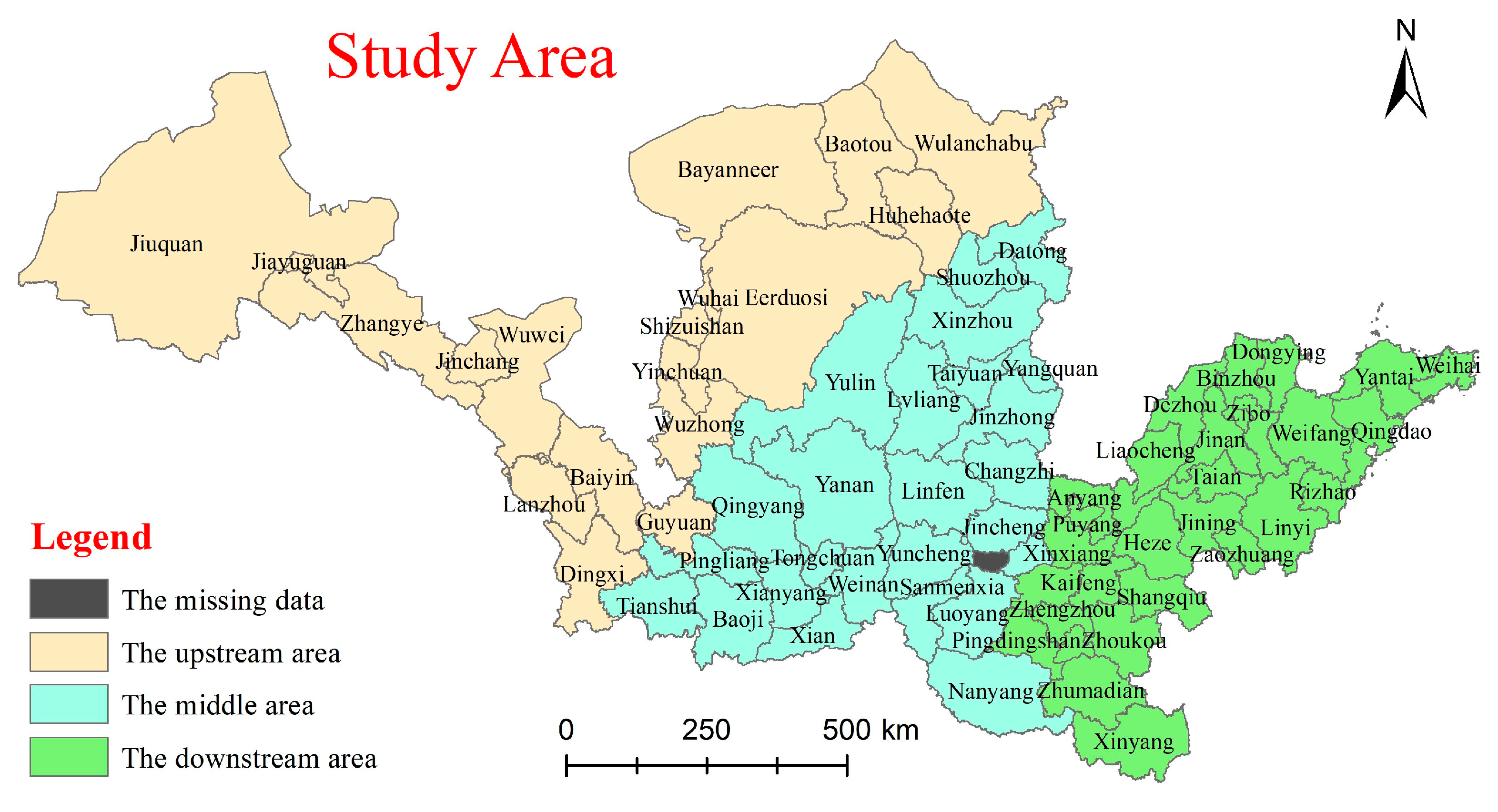
For this study, 73 prefecture-level cities in 9 provinces and autonomous regions of the Yellow River Basin were selected as the study area (Figure 1), and the time range of the data was 2000–2019. The relevant data came from the “China Statistical Yearbook”, the “China Agricultural Yearbook”, the “China Rural Statistical Yearbook”, the “Sixty Years of New China Statistical Data Compilation”, the “China Environmental Statistical Yearbook”, and the statistical yearbooks and statistical bulletins of various provinces and cities; the data of some missing years were supplemented by the mean of the sum of the values of adjacent years.

3. Results Analysis

3.1. Calculation Results of $AW{F}_{grey}$

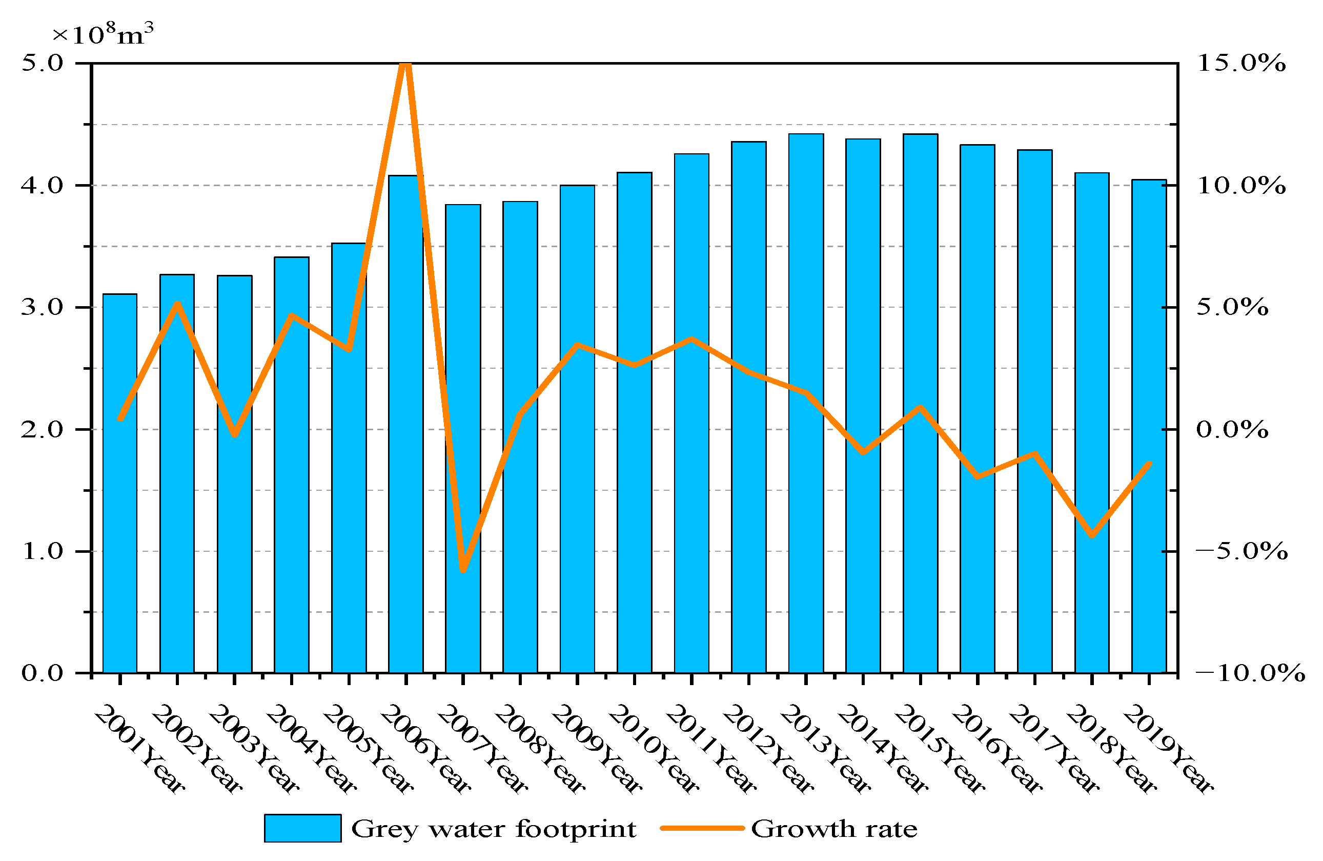
On the whole, taking 2015 as the study period, the $AW{F}_{grey}$ in the Yellow River Basin showed a trend of first rising and then falling (Figure 2). Among them, 2001−2006 was a period of rapid increase, where the average value of the $AW{F}_{grey}$ increased sharply from 3.1 × 10⁸ m³ to 4.1 × 10⁸ m³, with an average annual growth rate of about 6.25%. From 2006 to 2015, it first decreased sharply and then increased slowly. The average $AW{F}_{grey}$ first dropped sharply from 4.1 × 10⁸ m³ to 3.8 × 10⁸ m³ and then slowly climbed to 4.4 × 10⁸ m³, an increase of 0.6 × 10⁸ m³, with an average annual growth rate about 1.88%. From 2015 to 2019, there was a slow decline period. The average value of the $AW{F}_{grey}$ decreased from 4.4 × 10⁸ m³ to 4.0 × 10⁸ m³, with an average annual reduction rate of about 2.12%.

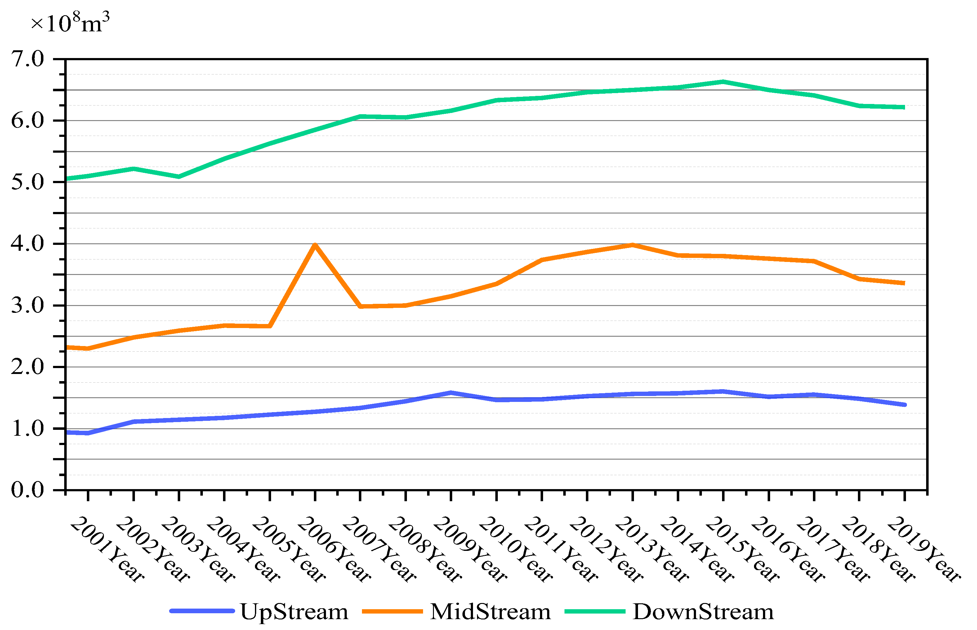
From the perspective of changes in different sections of the basin (Figure 3), the initial level of the $AW{F}_{grey}$ in the upper reaches of the Yellow River Basin was the lowest, and the multi−year average was stable at 1.4 × 10⁸ m³; the midstream regions were second, and the multi−year average was stable at 3.2 × 10⁸ m³; the downstream area was the highest, and the multi-year average was stable at 6.0 × 10⁸ m³, which is much larger than the sum of the $AW{F}_{grey}$ in the middle and upper reaches. However, the $AW{F}_{grey}$ in the upstream and midstream regions changed rapidly during the study period, with an average annual growth rate of about 2.39% and 2.28%, respectively, while the downstream region growth rate was only 1.27%. In 2006, the first pollution source census conducted in China found that the concentrations of pollutants such as COD MN and NH₃-N in the middle reaches of the Yellow River Basin were relatively high, and they flowed downstream along the river, resulting in serious downstream pollution. The region still has a long way to go in improving agricultural non-point source pollution.

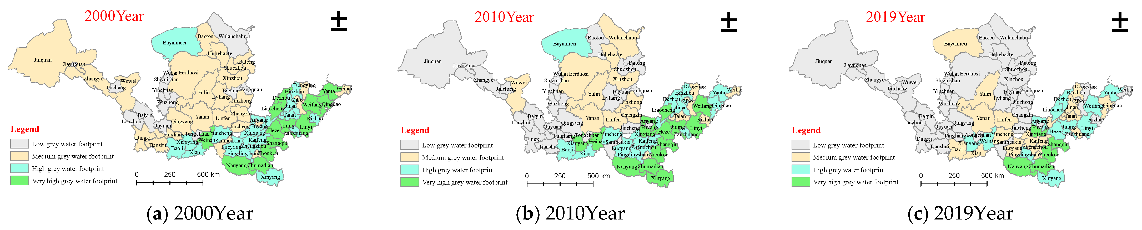
Further, based on the natural breakpoint method, the $AW{F}_{grey}$ of prefecture-level cities in the Yellow River Basin from 2000 to 2019 is divided into four groups: low, medium, high, and very high. (

Table 2. Threshold ranges of $AW{F}_{grey}$ in low, medium, high and very high groups (10⁶ m³).

Groups	2000	2010	2019
Low $AW{F}_{grey}$ group	[2.2, 74.3]	[3.0, 169.9]	[0.63, 252.3]
Medium $AW{F}_{grey}$ group	[74.3, 267.1]	[169.9, 371.8]	[252.3, 574.8]
High $AW{F}_{grey}$ group	[267.1, 562.0]	[371.8, 725.7]	[574.8, 905.2]
Very high $AW{F}_{grey}$ group	[562.0, 1038.9]	[725.7, 1399.9]	[905.2, 1579.0]

). By drawing the spatial distribution map of the $AW{F}_{grey}$ in the Yellow River Basin from 2000 to 2019 (Figure 4), it can be seen that, from 2000 to 2010, the overall spatial distribution pattern of the $AW{F}_{grey}$ in the Yellow River Basin remained unchanged; however, the number of prefecture-level cities included in the low group and medium groups changed significantly. Specifically, the number of prefecture-level cities in the low group increased rapidly from 13 to 26, an increase of 100.00%; the number of prefecture-level cities in the middle group decreased from 27 to 16, a decrease of 40.74%; the number of prefecture-level cities in the high group decreased from 20 to 17, a decrease of 15.00%; and the number of prefecture-level cities in the very-high group increased from 13 to 14, an increase of 7.69%.

From 2010 to 2019, the overall spatial distribution pattern of the $AW{F}_{grey}$ in the Yellow River Basin remained unchanged, but the number of prefecture-level cities included in the low and very-high groups changed significantly. Specifically, the number of prefecture-level cities in the low group increased rapidly from 26 to 36, an increase of 38.46%; the number of prefecture-level cities in the middle group increased from 16 to 19, an increase of 18.75%; the number of prefecture-level cities in the high group decreased from 17 to 13, a decrease of 23.53%; and the number of prefecture-level cities in the very high group decreased from 14 to 5, a decrease of 64.29%, indicating that the $AW{F}_{grey}$ in the Yellow River Basin decreased significantly and the ecological environment improved significantly.

3.2. Spatial and Temporal Characteristics of the $AW{F}_{grey}$ in the Yellow River Basin

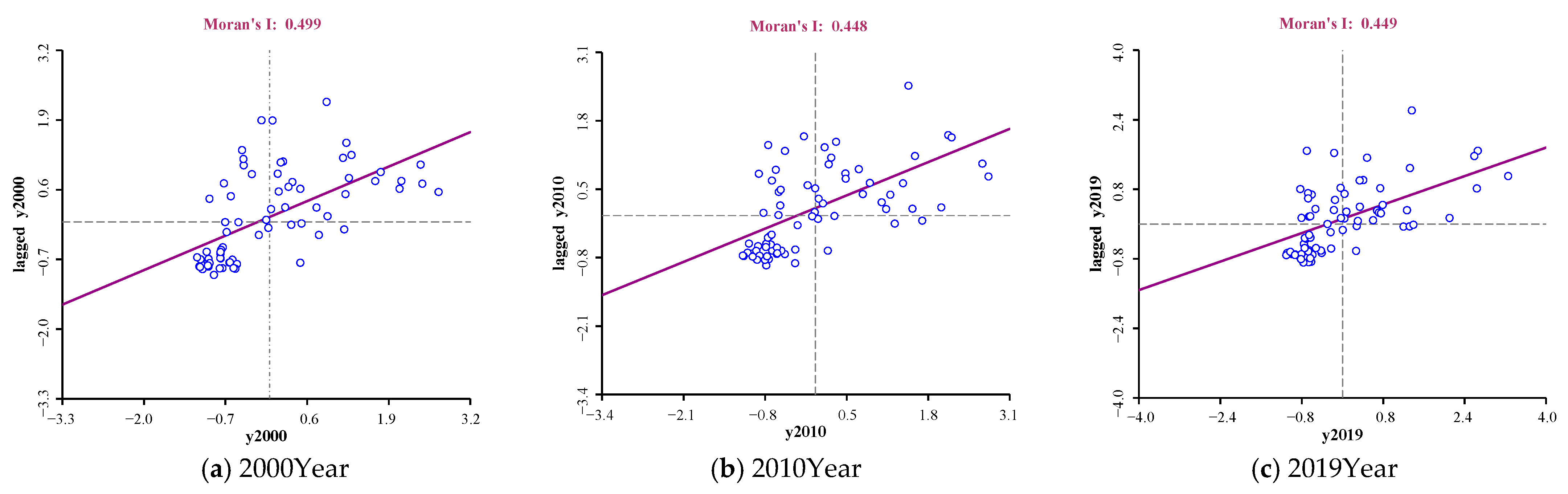
This study calculated the global autocorrelation Moran’s I index of the $AW{F}_{grey}$ of cities in the Yellow River Basin from 2000 to 2019. Due to space limitations, only the global Moran’s I index for 2000, 2010, and 2019 is shown (Figure 5). The $AW{F}_{grey}$ of the Yellow River Basin has shown a significant positive correlation in the past 20 years, that is, the areas with a high $AW{F}_{grey}$ are adjacent and the areas with a low $AW{F}_{grey}$ are also adjacent, showing obvious spatial agglomeration. The value of Moran’s I from 2000 to 2019 decreased slightly with the change in years, from 0.494 to 0.449, indicating that with the continuous development of the agricultural economy in the Yellow River Basin, the development speed of different regions has been inconsistent and the gap large. Therefore, the spatial agglomeration degree of the $AW{F}_{grey}$ has been slightly weakened.

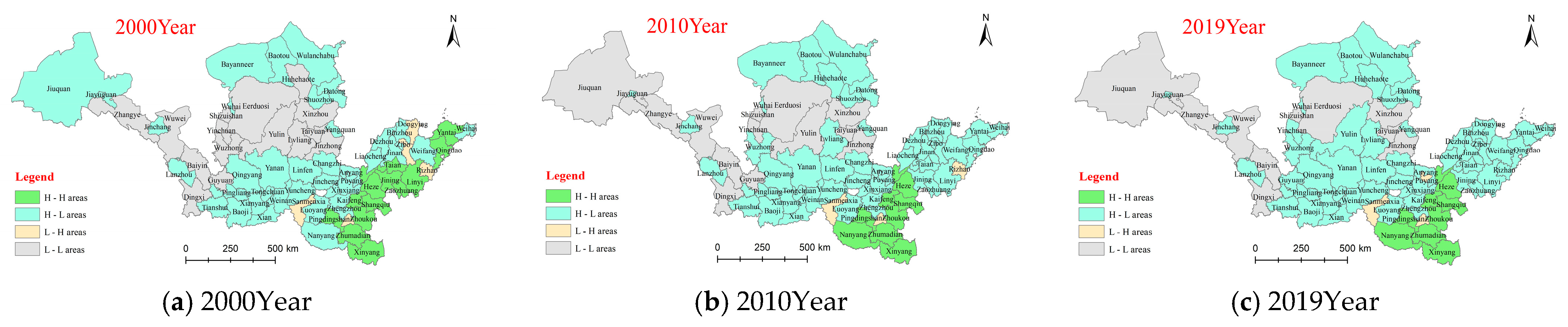
As the global Moran’s I index is an overall autocorrelation statistic, which represents whether the elements are distributed with significant aggregation or separation at the overall level, it cannot reveal the spatial agglomeration degree of specific regions. The LISA agglomeration map is a clearer visual expression of the local Moran’s I scatter plot. Analyzing the LISA agglomeration map can help to identify the “hot spot” and “blind spot” areas of the $AW{F}_{grey}$ in the Yellow River Basin and intuitively represent the local characteristics of the $AW{F}_{grey}$ in spatial distribution. Therefore, in this study, typical years were selected and LISA clustering maps were drawn for the $AW{F}_{grey}$ for each prefecture-level city in the Yellow River Basin in 2000, 2010, and 2019 (Figure 6).

From 2000 to 2010, the number of prefecture-level cities with H–L agglomerations in the $AW{F}_{grey}$ of the Yellow River Basin increased slightly, while the number of H–H, L–H, and L–L agglomerations decreased slightly. Specifically, the number of prefecture-level cities with H–L agglomeration increased from 38 to 47, an increase of 23.68%. The number of prefecture-level cities with H–H agglomeration decreased from 14 to 9, a decrease of 35.71%; the number of prefecture- level cities with L–H agglomeration decreased from 5 to 3, a decrease of 40.00%; and the number of prefecture- level cities with L–L agglomeration decreased from 15 to 13, a decrease of 13.33%.

From 2010 to 2019, the number of prefecture-level cities with H–L agglomerations in the $AW{F}_{grey}$ of the Yellow River Basin slightly increased; the number of H–H and L–H agglomerations remains the same; while the number of L–L agglomerations decreased slightly. Specifically, the number of H–L prefecture-level cities increased from 47 to 50, an increase of 6.38%; the number of prefecture-level cities with H–H agglomeration remained unchanged at 5; the number of prefecture-level cities with L–H agglomeration remained unchanged at 3; while the number of prefecture-level cities with L–L agglomeration decreased from 13 to 10, a decrease of 23.08%.

Further, by classifying the spatiotemporal transition types of the $AW{F}_{grey}$ in 73 prefecture-level cities in the Yellow River Basin (

Table 3. LISA transition types of $AW{F}_{grey}$ of 73 prefecture-level cities in the Yellow River Basin from 2000 to 2019.

Transition Type	Time Division
	2000–2010	2010–2019
Type Ⅰ	HLt→LLt+1: Jiuquan	—
	LLt→HLt+1: Lvliang, Huhehaote, Wuzhong	LLt→HLt+1: Yulin, Yinchuan, Guyuan
Type Ⅱ	HHt→HLt+1: Qingdao, Zaozhuang, Yantai, Jining, Taian, Linyi	—
	HLt→HHt+1: Nanyang	—
Type Ⅲ	—	HLt→LHt+1: Hebi
	LHt→HLt+1: Zibo, Dongying	LHt→HLt+1: Rizhao
Type Ⅳ	The remaining 59 prefecture-level cities	The remaining 67 prefecture-level cities

), the most common transition type was generally transition type IV, that is, the $AW{F}_{grey}$ of the spatial unit itself and the adjacent area maintained the same level of change. In the two time periods, the spatial cohesion increased from 81.94% to 93.06%, indicating that the spatial structure change of the $AW{F}_{grey}$ in the Yellow River Basin has obvious path-dependent characteristics, and this characteristic is gradually strengthening. The next transition types are type II and type I, which reflect the influence of spatial proximity on the $AW{F}_{grey}$ in some areas. Type III has the least transition in both the region itself and its adjacent areas. From 2000 to 2010, there were only two prefecture levels in Zibo and Dongying. Two prefecture-level cities, Hebi and Rizhao, appeared from 2010 to 2019, which further verified their atypical characteristics.

From 2000 to 2010, Jiuquan belonged to H–L agglomeration; influenced by the surrounding prefecture-level cities, it passively transitioned from H–L agglomeration to L–L agglomeration. Lvliang, Huhehaote, and Wuzhong all belonged to L–L agglomeration areas, and the $AW{F}_{grey}$ was in a stable agglomeration state. Affected by their own $AW{F}_{grey}$, they took the initiative to transition from the original L–L agglomeration to H–L agglomeration. Qingdao, Zaozhuang, Yantai, Jining, Taian, and Linyi all belonged to H–H agglomeration areas, and the $AW{F}_{grey}$ was in a stable agglomeration state. Affected by their own $AW{F}_{grey}$, they took the initiative to transition from the original H–H agglomeration to H–L agglomeration. Nanyang belonged to H–L agglomeration; influenced by the surrounding prefecture-level cities, it passively transitioned from H–L agglomeration to H–H agglomeration. Zibo and Dongying all belonged to L–H agglomeration areas; influenced by the surrounding prefecture-level cities, they passively transitioned from L–H agglomeration to H–L agglomeration.

From 2010 to 2019, Yulin, Yinchuan, and Guyuan all belonged to L–L agglomeration areas, and the $AW{F}_{grey}$ was in a stable agglomeration state. Affected by their own $AW{F}_{grey}$, they took the initiative to transition from the original L–L agglomeration to H–L agglomeration. Hebei belonged to H–L agglomeration; influenced by the surrounding prefecture-level cities, it passively transitioned from H–L agglomeration to L–H agglomeration. Rizhao belonged to L–H agglomeration; influenced by the surrounding prefecture-level cities, it passively transitioned from L–H agglomeration to H–L agglomeration. In general, due to the different spatial correlation patterns of the $AW{F}_{grey}$ in different cities, the spillover effect of inter-provincial $AW{F}_{grey}$ may promote the convergence or differentiation of the $AW{F}_{grey}$ in various regions, and then affect the overall structure of the $AW{F}_{grey}$ spatial distribution in the Yellow River Basin.

3.3. Analysis of Influencing Factors of the $AW{F}_{grey}$

In this study, SPSS 27.0 (SPSS Inc., Chicago, IL, USA) was used to test the normal distribution of the spatiotemporal series data of the $AW{F}_{grey}$ in the Yellow River Basin. Due to the small sample size, the results obtained by the Shapiro–Wilk Test were Sig = 0.275 and Sig = 0.266, which are both greater than 0.05 and obey normality. Therefore, the path analysis method could be used to study the temporal and spatial influencing factors of the $AW{F}_{grey}$ in the Yellow River Basin. From 2000 to 2019, the analysis results of the influencing factors of the time series change of the $AW{F}_{grey}$ in the Yellow River Basin are shown in Table 2. As the spatial distribution pattern of the $AW{F}_{grey}$ in the Yellow River Basin was stable in different years, the dependent variable $AW{F}_{grey}$ and the mean value of the independent variable from 2000 to 2019 were calculated to analyze the influencing factors of the spatial distribution of the $AW{F}_{grey}$.

It can be seen from

Table 4. Analysis results of influencing factors of temporal variation of $AW{F}_{grey}$ in the Yellow River Basin.

Influencing Factors	Direct Path Factor	Indirect Path Factor												Total Influence Factor
		X1	X2	X3	X4	X5	X6	X7	X8	X9	X10	X11	X12
X1	−0.191		−0.521	−0.302	−0.281	0.074	−0.008	1.625	−0.033	−0.029	−0.002	−0.005	−0.001	0.325
X2	−0.537	−0.185		−0.307	−0.271	0.071	−0.007	1.583	−0.032	−0.028	−0.003	−0.006	−0.002	0.275
X3	0.310	0.186	0.532		0.273	−0.074	0.007	−1.641	0.032	0.028	0.004	0.006	0.002	−0.335
X4	−0.294	−0.183	−0.496	−0.288		0.072	−0.006	1.568	−0.032	−0.028	−0.001	−0.004	0.000	0.307
X5	−0.079	0.178	0.485	0.292	0.267		0.006	−1.694	0.031	0.027	0.004	0.007	0.003	−0.473
X6	0.021	0.076	0.175	0.106	0.089	−0.024		−0.663	0.016	0.015	−0.007	−0.006	−0.006	−0.207
X7	1.712	−0.181	−0.497	−0.297	−0.269	0.078	−0.008		−0.032	−0.028	−0.003	−0.006	−0.002	0.468
X8	−0.035	−0.181	−0.494	−0.284	−0.269	0.069	−0.010	1.544		−0.031	−0.003	−0.005	−0.002	0.299
X9	−0.033	−0.168	−0.457	−0.261	−0.250	0.064	−0.010	1.430	−0.033		−0.003	−0.005	−0.002	0.271
X10	0.023	0.020	0.077	0.047	0.014	−0.014	−0.007	−0.222	0.005	0.005		0.021	0.017	−0.012
X11	0.022	0.042	0.137	0.084	0.049	−0.024	−0.006	−0.431	0.008	0.008	0.022		0.018	−0.068
X12	0.018	0.014	0.055	0.037	0.007	−0.014	−0.007	−0.194	0.003	0.004	0.022	0.022		−0.032

that the absolute values of the direct path coefficients of the factors affecting the time series changes of the $AW{F}_{grey}$ in the Yellow River Basin are $X_7$, $X_2$, $X_3$, $X_4$, $X_1$, $X_5$, $X_8$, $X_9$, $X_{10}$, $X_{11}$, $X_6$, and $X_{12}$, indicating that crop yield, economic scale, and urban and rural structure have a great direct impact on the $AW{F}_{grey}$, and the direct path coefficients are 1.712, −0.537, and 0.310, respectively. However, the direct influence of pesticide application intensity, resource endowment, and agricultural film application intensity are small, and the direct path coefficients are 0.022, 0.021, and 0.018, respectively. Through the analysis of the indirect path coefficient between the influencing factors, it can be concluded that each influencing factor has a great impact on the $AW{F}_{grey}$ according to crop yield, economic scale, urban and rural structure, and technological innovation. In terms of crop yield, population scale has a strong positive impact on the increase in the $AW{F}_{grey}$, while industrial structure has a strong negative impact on the increase in the $AW{F}_{grey}$ according to the crop yield. In terms of economic scale, the urban and rural structure has a strong positive impact on the increase in the $AW{F}_{grey}$, while population scale has a strong negative impact on the increase in the $AW{F}_{grey}$ according to the economic scale. In terms of urban and rural structure, the industrial structure has a strong positive impact on the increase in the $AW{F}_{grey}$, while the economic scale has a strong negative impact on the increase in the $AW{F}_{grey}$ according to the urban and rural structure. In terms of technological innovation, the urban and rural structure has a strong positive impact on the increase in the $AW{F}_{grey}$, while population scale has a strong negative impact on the increase in the $AW{F}_{grey}$ according to the technological innovation. Industrial structure and crop yield have the largest total influence on the $AW{F}_{grey}$, with the total influence coefficients of −0.473 and 0.468, respectively.

It can be seen from

Table 5. Analysis results of influencing factors of spatial variation of $AW{F}_{grey}$ in the Yellow River Basin.

Influencing Factors	Direct Path Factor	Indirect Path Factor												Total Influence Factor
		X1	X2	X3	X4	X5	X6	X7	X8	X9	X10	X11	X12
X1	0.355		0.004	0.019	0.275	−0.018	0.054	0.245	0.007	−0.001	0.000	0.004	0.001	0.947
X2	−0.026	−0.054		−0.029	0.041	0.003	−0.004	0.010	0.024	0.034	0.011	0.014	0.036	0.060
X3	0.077	0.087	0.010		0.114	−0.046	0.025	0.089	0.002	−0.005	−0.014	−0.004	−0.011	0.323
X4	0.369	0.265	−0.003	0.024		−0.035	0.041	0.247	0.015	0.009	0.004	0.003	0.010	0.949
X5	−0.071	0.091	0.001	0.050	0.181		0.030	0.117	0.012	0.011	−0.012	−0.003	0.003	0.411
X6	0.081	0.239	0.001	0.023	0.186	−0.026		0.151	0.009	0.007	−0.006	0.003	0.001	0.668
X7	0.284	0.307	−0.001	0.024	0.321	−0.029	0.043		0.017	0.014	0.006	0.007	0.018	1.010
X8	−0.057	−0.045	0.011	−0.003	−0.097	0.015	−0.012	−0.085		−0.061	−0.010	−0.011	−0.040	−0.395
X9	−0.074	0.004	0.012	0.005	−0.046	0.011	−0.007	−0.055	−0.047		−0.007	−0.016	−0.049	−0.267
X10	0.066	0.000	−0.004	−0.017	0.024	0.012	−0.007	0.024	0.009	0.007		0.006	0.007	0.128
X11	0.033	0.048	−0.011	−0.010	0.030	0.007	0.006	0.057	0.020	0.035	0.013		0.055	0.284
X12	0.103	0.005	−0.009	−0.008	0.035	−0.002	0.001	0.049	0.022	0.035	0.005	0.018		0.252

that the absolute values of the direct path coefficients of the factors affecting the spatial variation of the $AW{F}_{grey}$ in the Yellow River Basin are $X_4$, $X_1$, $X_7$, $X_{12}$, $X_6$, $X_3$, $X_9$, $X_5$, $X_{10}$, $X_8$, $X_{11}$, and $X_2$, indicating that technological innovation, population size, and crop yield have a strong direct impact on the $AW{F}_{grey}$, with the direct path coefficients being 0.369, 0.355, and 0.284, respectively. However, the direct effects of planting structure, pesticide application intensity, and economic scale are relatively small, with the direct path coefficients being −0.057, 0.033, and −0.026, respectively. According to the analysis of the indirect path coefficients of the influencing factors, it can be concluded that each influencing factor has a strong impact on the $AW{F}_{grey}$ according to economic scale, crop yield, population scale, and resource endowment. Among these, in terms of economic scale, crop yield has a strong positive impact on the increase in the $AW{F}_{grey}$, while planting structure has a strong negative impact on the increase in the $AW{F}_{grey}$ according to the economic scale. In terms of crop yield, population scale has a strong positive impact on the increase in the $AW{F}_{grey}$, while planting structure has a strong negative impact on the increase in the $AW{F}_{grey}$ according to the crop yield. In terms of population size, crop yield has a strong positive impact on the increase in the $AW{F}_{grey}$, while economic scale has a strong negative impact on the increase in the $AW{F}_{grey}$ according to the population size. In terms of resource endowment, population size has a strong positive impact on the increase in the $AW{F}_{grey}$, while planting structure has a strong negative impact on the increase in the $AW{F}_{grey}$ according to the resource endowment. Technological innovation, population size, and resource endowment have the largest total impact on the $AW{F}_{grey}$, with total impact coefficients of 0.949, 0.947, and 0.668, respectively.

4. Conclusions and Suggestions

4.1. Conclusions

In order to provide a scientific decision-making basis for the sustainable utilization of water resources and green development of agriculture in the Yellow River Basin, the temporal and spatial variation characteristics and influencing paths of the agricultural grey water footprint were studied in this paper. The main conclusions are as follows:

(1)

Based on the water footprint theory, the $AW{F}_{grey}$ of the Yellow River Basin from 2000 to 2019 was calculated. Taking 2015 as the study period, the results showed that the $AW{F}_{grey}$ of the Yellow River Basin had a trend of rising first and then falling. The values and growth rates of the $AW{F}_{grey}$ in different regions were quite different. The downstream value was much higher than that of the middle and upper reaches, but the growth rate was lower than that of the middle and upper reaches. In terms of temporal variation, the thresholds of the low, medium, high, and very-high $AW{F}_{grey}$ groups increased, while the proportion of prefecture-level cities in the high and very-high $AW{F}_{grey}$ groups decreased. In terms of spatial distribution, the low-$AW{F}_{grey}$ group was mainly concentrated in the upper and middle reaches, the middle-$AW{F}_{grey}$ group was mainly concentrated in the middle and lower reaches, and the high- and very-high-$AW{F}_{grey}$ groups were mainly concentrated in the lower reaches and gradually decreased over time.

(2)

Based on the LISA agglomeration map, the spatial correlation characteristics of the $AW{F}_{grey}$ of the cities in the Yellow River Basin were analyzed. The results showed that the distribution of the $AW{F}_{grey}$ in the Yellow River Basin not only had continuity in time, but also had obvious spatial agglomeration, and this difference gradually decreased. Generally, the “High–Low” agglomeration and the “Low–Low” agglomeration were dominant. From 2000 to 2019, most prefecture-level cities maintained the same transition changes as the neighboring regions. In the two time periods, spatial cohesion increased from 81.94% to 93.06%, indicating that the spatial structure change of the $AW{F}_{grey}$ in the Yellow River Basin had obvious path-dependent characteristics, and this characteristic was gradually strengthened.

(3)

Based on the path analysis method, the influencing factors of $AW{F}_{grey}$ spatial and temporal variation in the Yellow River Basin were analyzed. The results showed that crop yield, economic scale, and urban and rural structure were the main driving factors affecting the temporal variation of the $AW{F}_{grey}$ in the Yellow River Basin, and their direct path coefficients were 1.712, −0.537, and −0.310, respectively. Technological innovation, population size, and crop yield were the main influencing factors affecting the spatial distribution pattern, and their direct path coefficients were 0.369, 0.355, and 0.284, respectively. Crop yield was the only common factor influencing the spatio-temporal evolution of the $AW{F}_{grey}$ in the Yellow River Basin. Chen’s research holds that economic development and technological effects are the main negative and positive factors behind the decline in the grey water footprint, respectively [67]. In this study, economic scale was the main negative factor that leads to the increase in the agricultural grey water footprint. For the temporal change of the agricultural grey water footprint, scientific and technological innovation was the main negative factor that leads to the increase in the agricultural grey water footprint. Kong found that, according to the intensity and grey water footprint of Chinese provincial agriculture and the agricultural GDP, there was a growth inhibitory effect of the grey water footprint, and the driving role was determined [68]. In this study, we found the opposite conclusion in that economies of scale affected the main negative factors driving the temporal changes of the agricultural grey water footprint of the Yellow River. This may be caused by the study of the regional difference taking cities as the research object, so the scale was smaller and the results were more targeted.

4.2. Suggestions

Based on the above research conclusions, we proposed the following suggestions:

(1)

Appropriately control the population and the scale of agricultural economic development in the areas along the Yellow River Basin, and achieve balanced development between urban and rural areas. On the one hand, for the regions with a large population, the government should issue corresponding subsidy policies for out-migrating workers based on the actual situation of the city, and encourage a large number of young people to work and do business in the eastern region. On the other hand, for the regions with a small population, the government should strengthen the construction of living facilities for the residents, improve the level of education and medical care, reduce the cost of living, and attract people from other provinces to settle in this area, in order to realize the overall development of urban and rural areas in the Yellow River Basin.

(2)

Based on regional resource endowments, the layout of agricultural production should be optimized and the agricultural planting structure should be rationally adjusted to maximize the efficiency of grain output. Each region should build important agricultural production bases with distinctive advantages according to their regional resource endowments. Furthermore, the layout of agricultural production should be optimized and the agricultural planting structure should be rationally adjusted to maximize the scale efficiency of grain production, thereby reducing the agricultural grey water footprint, and accelerating the high-quality development of various agricultural regions.

(3)

Rely on the progress of agricultural science and technology to develop environment-friendly agriculture. Specifically, it is necessary to call on all municipal agricultural technology centers to hold online training courses on chemical fertilizer and pesticide reduction and efficiency enhancement technologies to guide farmers on how to popularize and apply “soil testing and formula fertilization technology” according to the fertilizer requirements of different crops. In addition, the National Agricultural Technology Center can also conduct training courses in various cities to demonstrate the relevant techniques to farmers and encourage them to observe and communicate, so as to explore new technologies for reducing chemical fertilizers and pesticides.

While offering a new perspective on evaluating agricultural water environment pollution in the Yellow River Basin, our study has limitations that represent opportunities for further research. First, due to the current academic circles not having reached a unified view on the definition of or calculation methods for the total agricultural grey water footprint (including planting, livestock, poultry breeding, and aquaculture, as well as data limitations), when calculating the agricultural grey water footprint, we only considered the grey water footprint produced by the application of chemical fertilizers (nitrogen fertilizers and compound fertilizers) in the planting industry. This may lead to a conservative value of the calculated agricultural grey water footprint. Second, through an empirical analysis, it was concluded that the agricultural grey water footprint of different regions in the Yellow River basin has differences in the spatial scale, but how does the spatial differences evolve? Will the gap in the agricultural grey water footprint of different regions converge over time? If so, what kind of convergence will it show? Due to the limitations of space and the focus of this paper, we have not yet discussed these issues yet. In the future, spatial convergence and other models will be introduced to further analyze these issues.

References

- Fan, G.Q.; Zhang, D.Z.; Zhang, J.M.; Li, Z.; Sang, W.; Zhao, L.; Xu, M. Ecological environmental effects of Yellow River irrigation revealed by isotope and ion hydrochemistry in the Yinchuan Plain, Northwest China. Ecol. Indic. 2022, 135, 108574. [Google Scholar] [CrossRef]
- Fang, L.N.; Yin, C.B.; Fang, Z.; Zhang, Y. The promotion path of high-quality development of agriculture in the Yellow River Basin. Chin. J. Agric. Resour. Reg. Plan. 2021, 42, 16–22. [Google Scholar]
- Lu, C.P.; Ji, W.; Hou, M.C.; Ma, T.; Mao, J. Evaluation of efficiency and resilience of agricultural water resources system in the Yellow River Basin, China. Agric. Water Manag. 2022, 266, 107605. [Google Scholar] [CrossRef]
- Zhang, N.N.; Su, X.L.; Zhou, Y.Z.; Niu, J.-P. Water resources carrying capacity evaluation of the Yellow River Basin based on EFAST weight algorithm. J. Nat. Resour. 2019, 34, 1759–1770. [Google Scholar] [CrossRef]
- Tao, Y.; Xu, J.; Ren, H.J.; Guan, X.; You, L.; Wang, S. Spatiotemporal evolution of agricultural non-point source pollution and its influencing factors in the Yellow River Basin. Trans. Chin. Soc. Agric. Eng. 2021, 37, 257–264. [Google Scholar]
- Ercin, A.E.; Aldaya, M.M.; Hoekstra, A.Y. Corporate Water Footprint Accounting and Impact Assessment: The Case of the Water Footprint of a Sugar-Containing Carbonated Beverage. Water Resour. Manag. 2011, 25, 721–741. [Google Scholar] [CrossRef]
- Hoekstra, A.Y.; Chapagain, A.K.; Aldaya, M.M.; Mekonnen, M.M. The Water Footprint Assessment Manual; Science Press: Beijing, China, 2012. [Google Scholar]
- Ren, Z.A.; Rong, J.R. Decoupling Relationship Between Utilization of Water Resource and Economic Growth in Anhui. J. Heilonjiang Univ. Technol. 2017, 17, 58–63. [Google Scholar]
- Wickramasinghe, W.M.S.; Navaratne, C.M.; Dias, S.V. Building resilience on water quality management through grey water footprint approach: A case study from Sri Lanka. Procedia Eng. 2018, 212, 752–759. [Google Scholar] [CrossRef]
- Hong, C.C.; Liu, M.C.; Zhang, Y.J.; Wu, L.Q. Analysis on the intensity and efficiency of agricultural grey water footprint in Beijing-Tianjin-Hebei Region under the perspective of spatial-temporal patten. J. Hebei Agric. Univ. 2021, 44, 128–135. [Google Scholar]
- Muratoglu, A. Grey water footprint of agricultural production: An assessment based on nitrogen surplus and high-resolution leaching runoff fractions in Turkey. Sci. Total Environ. 2020, 742, 140553. [Google Scholar] [CrossRef] [PubMed]
- Wu, M.Y.; Li, Y.Y.; Xiao, J.F.; Guo, X.; Cao, X. Blue, green, and grey water footprints assessment for paddy irrigation-drainage system. J. Environ. Manag. 2022, 302, 114116. [Google Scholar] [CrossRef] [PubMed]
- Feng, H.Y.; Sun, F.Y.; Liu, Y.Y.; Zeng, P.; Deng, L.; Che, Y. Mapping multiple water pollutants across China using the grey water footprint. Sci. Total Environ. 2021, 785, 147255. [Google Scholar] [CrossRef]
- Xie, D.; Zhuo, L.; Xie, P.X.; Liu, Y.; Feng, B.; Wu, P. Spatiotemporal variations and developments of water footprints of pig feeding and pork production in China (2004–2013). Agric. Ecosyst. Environ. 2020, 297, 106932. [Google Scholar] [CrossRef]
- Lin, J.W.; Weng, L.Y.; Dai, Y.H. Study on spatial and temporal pattern of grey water footprint and its decoupling relationship in China. Water Conserv. Sci. Technol. Econ. 2019, 25, 14–21. [Google Scholar]
- Li, C.H.; Xu, M.; Wang, X.; Tan, Q. Spatial analysis of dual-scale water stresses based on water footprint accounting in the Haihe River Basin, China. Ecol. Indic. 2018, 92, 254–267. [Google Scholar] [CrossRef]
- Ma, W.J.; Meng, L.H.; Wei, F.L.; Opp, C.; Yang, D. Spatiotemporal variations of agricultural water footprint and socioeconomic matching evaluation from the perspective of ecological function zone. Agric. Water Manag. 2021, 249, 106803. [Google Scholar] [CrossRef]
- Zhang, Y.; Tan, Q.; Zhang, T.Y.; Zhang, T.; Zhang, S. Sustainable agricultural water management incorporating inexact programming and salinization-related grey water footprint. J. Contam. Hydrol. 2022, 247, 103961. [Google Scholar] [CrossRef]
- Jamshidi, S.; Imani, S.; Delavar, M. An approach to quantifying the grey water footprint of agricultural productions in basins with impaired environment. J. Hydrol. 2022, 606, 127458. [Google Scholar] [CrossRef]
- Yang, Z.W.; Li, B.; Xia, R.; Ma, S.; Jia, R.; Ma, C.; Wang, L.; Chen, Y.; Bin, L. Understanding China’s industrialization driven water pollution stress in 2002–2015—A multi-pollutant based net gray water footprint analysis. J. Environ. Manag. 2022, 310, 114735. [Google Scholar] [CrossRef]
- He, Z.W.; Xiang, P.A. An Analysis of the Variations and Driving Factors of Grey Water Footprint in Hunan Province. China Rural Water Hydropower 2018, 10, 19–26. [Google Scholar]
- Li, H.; Liang, S.; Liang, Y.H.; Li, K.; Qi, J.; Yang, X.; Feng, C.; Cai, Y.; Yang, Z. Multi-pollutant based grey water footprint of Chinese regions. Resour. Conserv. Recycl. 2021, 164, 105202. [Google Scholar] [CrossRef]
- Li, X.C.; Chen, D.; Cao, X.; Luo, Z.; Webber, M. Assessing the components of, and factors influencing, paddy rice water footprint in China. Agric. Water Manag. 2020, 229, 105939. [Google Scholar] [CrossRef]
- Wang, Z.Y.; Xu, D.Y.; Peng, D.L.; Zhang, Y. Quantifying the influences of natural and human factors on the water footprint of afforestation in desert regions of northern China. Sci. Total Environ. 2021, 780, 146577. [Google Scholar] [CrossRef] [PubMed]
- Feng, B.B.; Liu, X.F.; Zhao, Y.G.; Li, K. Estimate of blue and green water footprint of crop production and analysis of its influencing factors in Shanxi province. Res. Soil Water Conserv. 2018, 25, 200–205, 214. [Google Scholar]
- Cai, J.P.; Xie, R.; Wang, S.J.; Deng, Y.; Sun, D. Patterns and driving forces of the agricultural water footprint of Chinese cities. Sci. Total Environ. 2022, 843, 156725. [Google Scholar] [CrossRef] [PubMed]
- Zhang, L.; Dong, H.J.; Geng, Y.; Francisco, M.J. China’s provincial grey water footprint characteristic and driving forces. Sci. Total Environ. 2019, 677, 427–435. [Google Scholar] [CrossRef]
- Hu, Y.; Huang, Y.; Tang, J.; Gao, B.; Yang, M.; Meng, F.; Cui, S. Evaluating agricultural grey water footprint with modeled nitrogen emission data. Resour. Conserv. Recycl. 2018, 138, 64–73. [Google Scholar] [CrossRef]
- Corredor, J.A.G.; González, G.L.V.; Granados, M.V.; Gutiérrez, L.; Pérez, E.H. Use of the gray water footprint as an indicator of contamination caused by artisanal mining in Colombia. Resour. Policy 2021, 73, 102197. [Google Scholar] [CrossRef]
- Liu, J.X.; Li, Y.; Zheng, Y.M.; Tong, S.; Zhang, X.; Zhao, Y.; Zheng, W.; Zhai, B.; Wang, Z.; Li, Z.; et al. The spatial and temporal distribution of nitrogen flow in the agricultural system and green development assessment of the Yellow River Basin. Agric. Water Manag. 2022, 263, 107425. [Google Scholar] [CrossRef]
- Tsaboula, A.; Papadakis, E.N.; Vryzas, Z.; Kotopoulou, A.; Kintzikoglou, K.; Papadopoulou-Mourkidou, E. Assessment and management of pesticide pollution at a river basin level part I: Aquatic ecotoxicological quality indices. Sci. Total Environ. 2019, 653, 1597–1611. [Google Scholar] [CrossRef]
- Chukalla, A.D.; Krol, M.S.; Hoekstra, A.Y. Grey water footprint reduction in irrigated crop production: Effect of nitrogen application rate, nitrogen form, tillage practice and irrigation strategy. Hydrol. Earth Syst 2018, 20, 3245–3259. [Google Scholar] [CrossRef]
- Wang, S.Y.; Lin, Y.J. Spatial Evolution and its Drivers of Regional Agro-ecological Efficiency in China’s from the Perspective of Water Footprint and Grey Water Footprint. Sci. Geogr. Sin. 2021, 41, 291–301. [Google Scholar]
- Han, Q.; Sun, C.Z.; Zou, W. Grey water footprint efficiency measure and its driving pattern analysis on provincial scale in China from 1998 to 2012. Resour. Sci. 2016, 38, 1179–1191. [Google Scholar]
- Wang, Y.Q.; Xian, C.F.; Ouyang, Z.Y. Integrated assessment of sustainability in urban water resources utilization in China based on grey water footprint. Acta Ecol. Sin. 2021, 41, 2983–2995. [Google Scholar]
- Ju, X.T.; Xing, G.X.; Chen, X.P.; Zhang, S.L.; Zhang, L.J.; Liu, X.J.; Cui, Z.L.; Yin, B.; Christie, P.; Zhu, Z.L.; et al. Reducing environmental risk by improving N management in intensive Chinese agricultural systems. Proc. Natl. Acad. Sci. USA 2009, 106, 3041–3046. [Google Scholar] [CrossRef] [PubMed]
- Mekonnen, M.M.; Hoekstra, A.Y. The green, blue and grey water footprint of crops and derived crop products. Hydrol. Earth Syst. 2011, 15, 1577–1600. [Google Scholar] [CrossRef]
- De Girolamo, A.M.; Miscioscia, P.; Politi, T.; Barca, E. Improving grey water footprint assessment: Accounting for uncertainty. Ecol. Indic. 2019, 102, 822–833. [Google Scholar] [CrossRef]
- Ma, F.C.; Liu, Q.N. Spatial Correlation Pattern and Influencing Factors of “Water Footprint Intensity of Grain Crops” in Heilongjiang Province. Ecol. Econ. 2021, 37, 121–127, 144. [Google Scholar]
- Sun, L. Spatial Empirical Study on Regional Differences and Influencing Factors of Water Footprint Intensity in China; South China University of Technology: Guangzhou, China, 2017. [Google Scholar]
- Kumari, M.; Sarma, K.; Sharma, R. Using Moran’s I and GIS to study the spatial pattern of land surface temperature in relation to land use/cover around a thermal power plant in Singrauli district, Madhya Pradesh, India. Remote Sens. Appl. Soc. Environ. 2019, 15, 100239. [Google Scholar] [CrossRef]
- Tepanosyan, G.; Sahakyan, L.; Zhang, C.S.; Saghatelyan, A. The application of Local Moran’s I to identify spatial clusters and hot spots of Pb, Mo and Ti in urban soils of Yerevan. Appl. Geochem. 2019, 104, 116–123. [Google Scholar] [CrossRef]
- Zhang, Y.Q.; Rashid, A.; Guo, S.S.; Jing, Y.; Zeng, Q.; Li, Y.; Adyari, B.; Yang, J.; Tang, L.; Yu, C.-P.; et al. Spatial autocorrelation and temporal variation of contaminants of emerging concern in a typical urbanizing river. Water Res. 2022, 212, 118120. [Google Scholar] [CrossRef] [PubMed]
- Melecky, L. Spatial Autocorrelation Method for Local Analysis of the EU. Procedia Econ. Financ. 2015, 23, 1102–1109. [Google Scholar] [CrossRef]
- Xiao, Y.X.; Gong, P. Removing spatial autocorrelation in urban scaling analysis. Cities 2022, 124, 103600. [Google Scholar] [CrossRef]
- Hou, M.Y.; Yao, S.B. Convergence and differentiation characteristics on agro-ecological efficiency in China from a spatial perspective. China Popul. Resour. Environ. 2019, 29, 116–126. [Google Scholar]
- Zhu, J.J.; Shi, X.Y. Analysis of Spatial Autocorrelation Patterns of Land Use and Influence Factors in Loess Hilly Region—A Case Study of Changhe Basin of Jincheng City. Res. Soil Water Conserv. 2018, 25, 234–241. [Google Scholar]
- Meng, B.; Wang, J.F.; Zhang, W.Z. Evaluation of Regional Disparity in China Based on Spatial Analysis. Sci. Geogr. Sin. 2005, 4, 11–18. [Google Scholar]
- Rey, S.J.; Janikas, M.V. Space-time analysis of regional systems. Geogr. Anal. 2006, 38, 67–86. [Google Scholar] [CrossRef]
- Song, W.; Chen, Y. Selection of observed variables and measuring indicators for the land use spatial autocorrelation analysis. J. Arid Land Resour. Environ. 2015, 29, 37–42. [Google Scholar]
- Ghalhari, G.F.; Roudbari, A.D. An investigation on thermal patterns in Iran based on spatial autocorrelation. Theor. Appl. Clim. 2018, 131, 865–876. [Google Scholar] [CrossRef]
- Ren, H.R.; Shang, Y.J.; Zhang, S. Measuring the spatiotemporal variations of vegetation net primary productivity in Inner Mongolia using spatial autocorrelation. Ecol. Indic. 2020, 112, 106108. [Google Scholar] [CrossRef]
- Lin, Z.; Chao, L.; Wu, C.Z.; Hong, W.; Hong, T.; Hu, X. Spatial analysis of carbon storage density of mid-subtropical forests using geostatistics: A case study in Jiangle County, southeast China. Acta Geochim. 2018, 37, 90–101. [Google Scholar] [CrossRef]
- Cao, X.C.; Shao, G.C.; Wang, X.J.; Wang, Z.; He, X.; Yang, C. Generalized water efficiency and strategic implications for food security and water management: A case study of grain production in China. Adv. Water Sci. 2017, 28, 14–21. [Google Scholar]
- Bi, D.D.; Wang, K.; Wang, L.J.; Fang, Y. Research on Industrial Eco-Efficiency and Spatio-Temporal Transition Characteristics of the Yangtze River Delta. Econ. Geogr. 2018, 38, 166–173. [Google Scholar]
- Zhao, G.M.; Zhao, G.Q.; Chen, L.Z. Research on spatial and temporal evolution of carbon emission intensity and its transition mechanism in China. China Popul. Resour. Environ. 2017, 27, 84–93. [Google Scholar]
- Tao, R.; Zhang, Q.Q.; Li, R.; Liu, T.; Chu, G.X. Response of roil N2O emission to partial chemical fertilizer substituted by organic fertilizer in mulch-drip irrigated cotton field. Trans. Chin. Soc. Agric. Mach. 2015, 46, 204–211. [Google Scholar]
- Cheng, W.T. Economic Decoupling and Water Use Efficiency Analysis Based on Water Footprint of Farming in Liaoning Province; Shenyang Agricultural University: Shenyang, China, 2020. [Google Scholar]
- Zong, R.; Wang, Z.H.; Zhang, J.Z.; Li, W. The response of photosynthetic capacity and yield of cotton to various mulching practices under drip irrigation in Northwest China. Agric. Water Manag. 2021, 249, 106814. [Google Scholar] [CrossRef]
- Yu, S.W.; Zhu, K.J.; Zhang, X. Energy demand projection of China using a path-coefficient analysis and PSO–GA approach. Energy Convers. Manag. 2012, 53, 142–153. [Google Scholar] [CrossRef]
- Jia, L.J.; Fan, D.C.; Wu, Y.J. Research on industrial structural adjustment under the background of low carbon economy. Inq. Into Econ. Issues 2013, 2, 87–92. [Google Scholar]
- Song, C.M.; Li, C.G.; Xiang, Y.L. Study on energy consumption’s determinants based on path analysis. J. Arid Land Resour. Environ. 2012, 26, 174–179. [Google Scholar]
- Li, Y.P.; Wu, W.N.; Yang, J.X.; Cheng, K.; Smith, P.; Sun, J.; Xu, X.; Yue, Q.; Pan, G. Exploring the environmental impact of crop production in China using a comprehensive footprint approach. Sci. Total Environ. 2022, 824, 153898. [Google Scholar] [CrossRef]
- Zhao, J.C.; Han, T.; Wang, C.; Shi, X.; Wang, K.; Zhao, M.; Chen, F.; Chu, Q. Assessing variation and driving factors of the county-scale water footprint for soybean production in China. Agric. Water Manag. 2022, 263, 107469. [Google Scholar] [CrossRef]
- Wang, Y.; Zhang, Y.H.; Sun, W.X.; Zhu, L. The impact of new urbanization and industrial structural changes on regional water stress based on water footprints. Sustain. Cities Soc. 2022, 79, 103686. [Google Scholar] [CrossRef]
- Valis, D.; Hasilova, K.; Forbelska, M.; Pietrucha-Urbanik, K. Modelling water distribution network failures and deterioration. In Proceedings of the 2017 IEEE International Conference on Industrial Engineering and Engineering Management, Singapore, 10–13 December 2017; pp. 924–928. [Google Scholar] [CrossRef]
- Chen, J.; Gao, Y.Y.; Qian, H.; Jia, H.; Zhang, Q. Insights into water sustainability from a grey water footprint perspective in an irrigated region of the Yellow River Basin. J. Clean. Prod. 2021, 316, 128329. [Google Scholar] [CrossRef]
- Kong, Y.; He, W.J.; Zhang, Z.F.; Shen, J.; Yuan, L.; Gao, X.; An, M.; Ramsey, T.S. Spatial-temporal variation and driving factors decomposition of agricultural grey water footprint in China. J. Environ. Manag. 2022, 318, 115601. [Google Scholar] [CrossRef] [PubMed]
Figure 1.
Study area map.
Figure 2.
The overall evolution trend of in the Yellow River Basin.
Figure 3.
in the Upper, middle and lower Reaches of the Yellow River Basin from 2000 to 2019.
Figure 4.
Spatial distribution of the in the Yellow River Basin from 2000 to 2019.
Figure 5.
Moran’s index diagram of global autocorrelation of the of prefecture-level cities in the Yellow River Basin.
Figure 6.
LISA agglomeration and distribution of the of prefecture-level cities in the Yellow River Basin from 2000 to 2019.