
Comparative Study on Water Temperature Stratified Flow under Different Vertical Coordinate Systems in Delft3D

College of Water Science and Engineering, Taiyuan University of Technology, Taiyuan 030024, China
*
Author to whom correspondence should be addressed.
Water 2022, 14(17), 2737; https://doi.org/10.3390/w14172737
Submission received: 25 July 2022
/
Revised: 26 August 2022
/
Accepted: 31 August 2022
/
Published: 2 September 2022
(This article belongs to the Special Issue Hydraulics of River Networks and Modelling)
Abstract
:Reservoirs often suffer from water blooms, which are likely related to the hydrodynamic and water temperature characteristics of the tributary bays. To obtain the detailed changing process of hydrodynamics and water temperature stratification, it is necessary to choose a suitable vertical coordinate system in order to achieve the required precision. Based on a physical model experiment of cold water flowing into the Generalized Reservoir Hydraulics (GRH) flume, both the σ-coordinate system model and the z-coordinate system model are built for comparison. For the z-coordinate system model, the influences of different grid resolutions and different bottom slopes on the simulation accuracy are also analyzed. The results show that the σ-coordinate system model can simulate cold-water underflow in a reservoir better than the z-coordinate system model, and the numerical errors of the z-coordinate system model can be reduced but not eliminated by increasing the horizontal grid resolution. When the bottom slope of the reservoir is less than 18‰, the z-coordinate system model can also be used to simulate cold-water underflow in a reservoir. The conclusions about vertical coordinate systems can be applied to the development of a three-dimensional hydrodynamic and water temperature model of reservoirs.
1. Introduction
Since the impoundment of the Three Gorges Reservoir (TGR), water blooms frequently occur in several tributary bays, which has aroused widespread public concern [1,2,3]. Some studies have suggested that water temperature stratification and density flow are the main causes of water blooms in these tributary bays [4,5,6,7,8]. Previous field observations and numerical simulations show that the hydrodynamic exchange process between the tributary bays and the Yangtze River provides rich nutrients and suitable hydrodynamic conditions for algae growth [9,10,11,12,13]. Therefore, the hydrodynamic and water temperature characteristics in the tributary bays are important to explain the mechanism of water blooms [14]. Numerical simulation is an economical and practical method to obtain the hydrodynamic characteristics and water temperature stratification in the tributary bays. The Delft3D model is widely used for the numerical simulation of gravity flow in reservoirs and estuaries, and it is employed to build the three-dimensional hydrodynamic and water temperature numerical models in this study.
Generally, there are the following two common types of vertical coordinate systems in Delft3D when building a three-dimensional model: one is the z-coordinate system, and the other is the σ-coordinate system [15]. The σ-coordinate system model is a boundary-fitted model that can simulate the changes in the bottom and free surface. For a steep bottom slope in combination with vertical water temperature stratification, the σ-coordinate system model introduces artificial vertical diffusion due to truncation errors in the approximation of the horizontal pressure gradient force [16,17,18]. The z-coordinate system model has horizontal grid lines and is not boundary-fitted in the vertical direction. The bottom and free surface are represented as a staircase, which causes numerical errors in bed shear stress. Improvement methods such as anti-creep correction for the σ-coordinate system model [19] and remapping of near-bottom layers for the z-coordinate system model [20] cannot completely eliminate these errors. Therefore, when simulating density flow in a water temperature stratified reservoir, the choice of the vertical coordinate system still needs to be taken into consideration.
In this study, based on the physical model experiment conducted by Johnson [21], two types of vertical coordinate systems are employed to establish two three-dimensional numerical models. According to the comparison of the two models with different grid resolutions and different bottom slopes, the application conditions of the two vertical coordinate systems are provided. This information is useful in determining a suitable vertical coordinate system when simulating density flow in a water temperature stratified reservoir.
2. Materials and Methods
The Delft3D model was developed by the Dutch institute for Delta Technology (Deltares) and can be used to simulate three-dimensional currents, waves, water quality, ecology, sediment, etc. The governing equation is the incompressible fluid N-S equation. Based on the shallow water assumption, the vertical acceleration in the vertical momentum equation is ignored, and the vertical flow velocity is obtained from the continuous equation. In the horizontal direction, an orthogonal curved mesh [22,23] was used in the earlier versions, and a non-structured mesh (Delft3D Flexible Mesh) has been presented in recent years. In the vertical direction, both the σ-coordinate system and the z-coordinate system can be chosen. To suppress artificial vertical diffusion and artificial flow due to truncation errors in the σ-coordinate system model, an anti-creep correction approach can be activated to approximate the horizontal diffusive fluxes and baroclinic pressure gradients in Cartesian coordinates by defining rectangular finite volumes around the σ-coordinate grid points. To avoid numerical errors due to the staircase representation of the bottom and free surface boundary in the z-coordinate system model, a near-bottom layers remapping approach is implemented, which can convert two near-bed layers into equidistant layering [24].
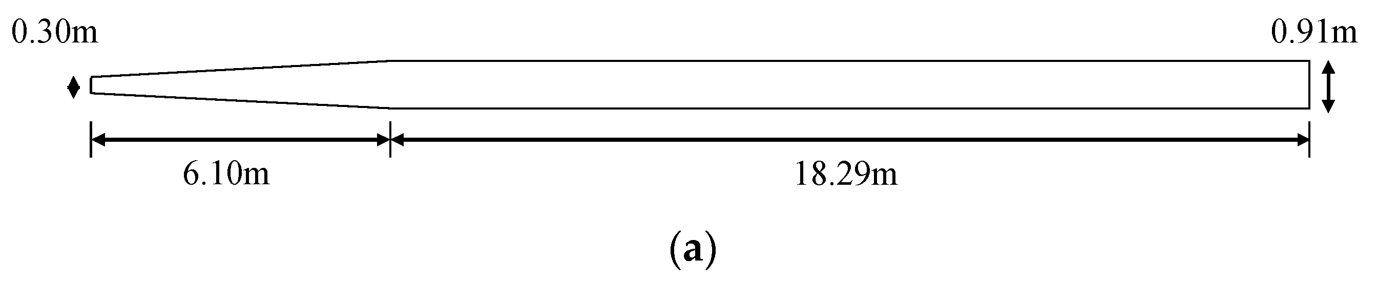
Considering the various uncertainties of actual field data, Johnson conducted a flume experiment about cold water flowing into the Generalized Reservoir Hydraulics (GRH) flume at the Waterways Experiment Station (WES) [21]. The water temperature and basic hydrodynamic data were obtained. A sketch of the experimental flume is shown in Figure 1. Its length is 24.39 m, the downstream section is 0.91 m × 0.91 m, and the upstream section is 0.30 m × 0.30 m. The reservoir can be divided into two parts. The upper reaches are 6.10 m in length and 0.30 m in depth, and the width changes linearly from 0.30 m to 0.91 m. The lower reaches are 18.29 m in length and 0.91 m in width, and the depth linearly changes from 0.30 m to 0.91 m. At the initial moment, the reservoir model was in a stationary state with a uniform water temperature of 21.44 °C. During the experiment, cold water at 16.67 °C was introduced into the reservoir at a position 0.46 m from the upstream section, and the baffle restricted cold water to the lower half (0.15 m × 0.30 m) of the section. The outlet was a hole with a diameter of 2.54 cm, located at the center line and 0.15 m above the floor at the downstream section. Both the inflow and outflow discharges were 0.00063 m3/s.
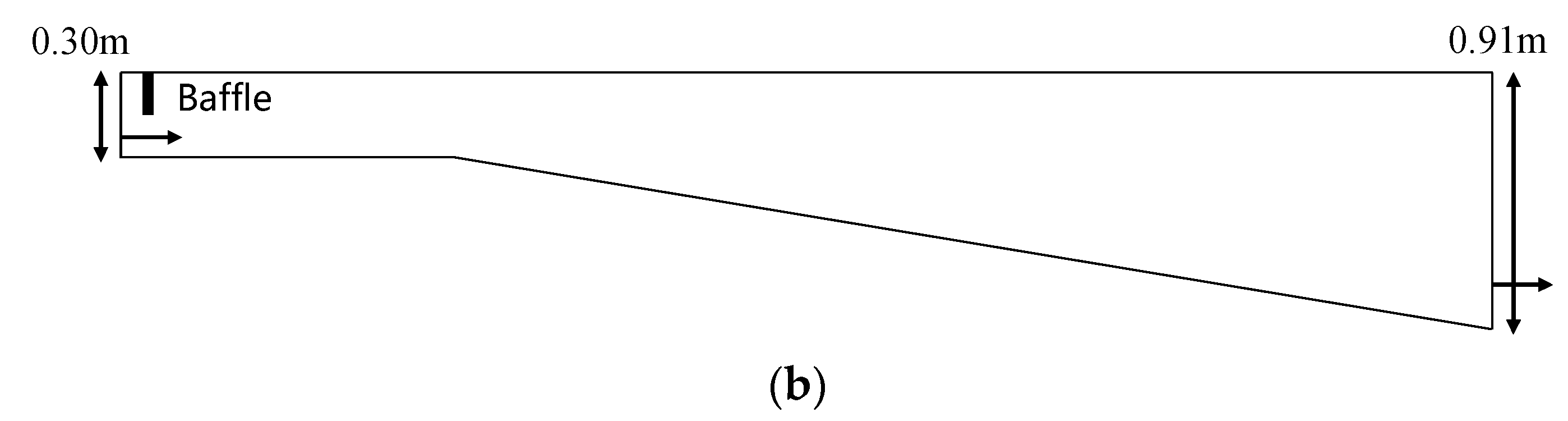
Three-dimensional numerical reservoir models of the σ-coordinate system and the z-coordinate system were both built for comparison. Moreover, methods to improve the simulation precision [24], such as anti-creep correction for the σ-coordinate system model and remapping of near-bottom layers for the z-coordinate system model, were also considered. Details of the simulation conditions are listed in Table 1. The simulation time was 30 min, and the time step was 0.01 min for each simulation condition. The horizontal and vertical grid numbers of the two models remained the same, as did the model parameters. The turbulence model was the k-ε turbulence model, which had been successfully applied for the simulation of stratified flow in the Hong Kong waters [25] and verified for the seasonal evolution of the thermocline [26]. Details of the computational parameters are listed in Table 2. The vertical grids for different simulation conditions are displayed in Figure 2.
As shown in Figure 2, the vertical grid resolution of the σ-coordinate system model and the z-coordinate system model is different, although the vertical grid number of the two models is the same. In fact, the vertical grid resolution of the z-coordinate system model is always lower than that of the σ-coordinate system model when the two models have the same vertical grid number. Therefore, it is necessary to increase the vertical grid number of the z-coordinate system model in order to achieve the same grid resolution as the σ-coordinate system model. Considering the numerical errors caused by the staircase representation of boundaries in the z-coordinate system model, previous studies pointed out that increasing the horizontal grid number can better fit the bottom and free surface boundary [27,28]. Johnson’s experiment considered the process of cold water flowing into the reservoir along the bed, which means that the accuracy of bottom boundary approximation is significantly important. Therefore, the grid resolution of the z-coordinate system model should be studied to guarantee the simulation accuracy [29]. Five conditions with different grid resolutions were designed, as shown in Table 3. Conditions B1, B2, and B3 can be compared to study the influence of the vertical grid resolution, and conditions B1, B4, and B5 can be compared to study the influence of the horizontal grid resolution.
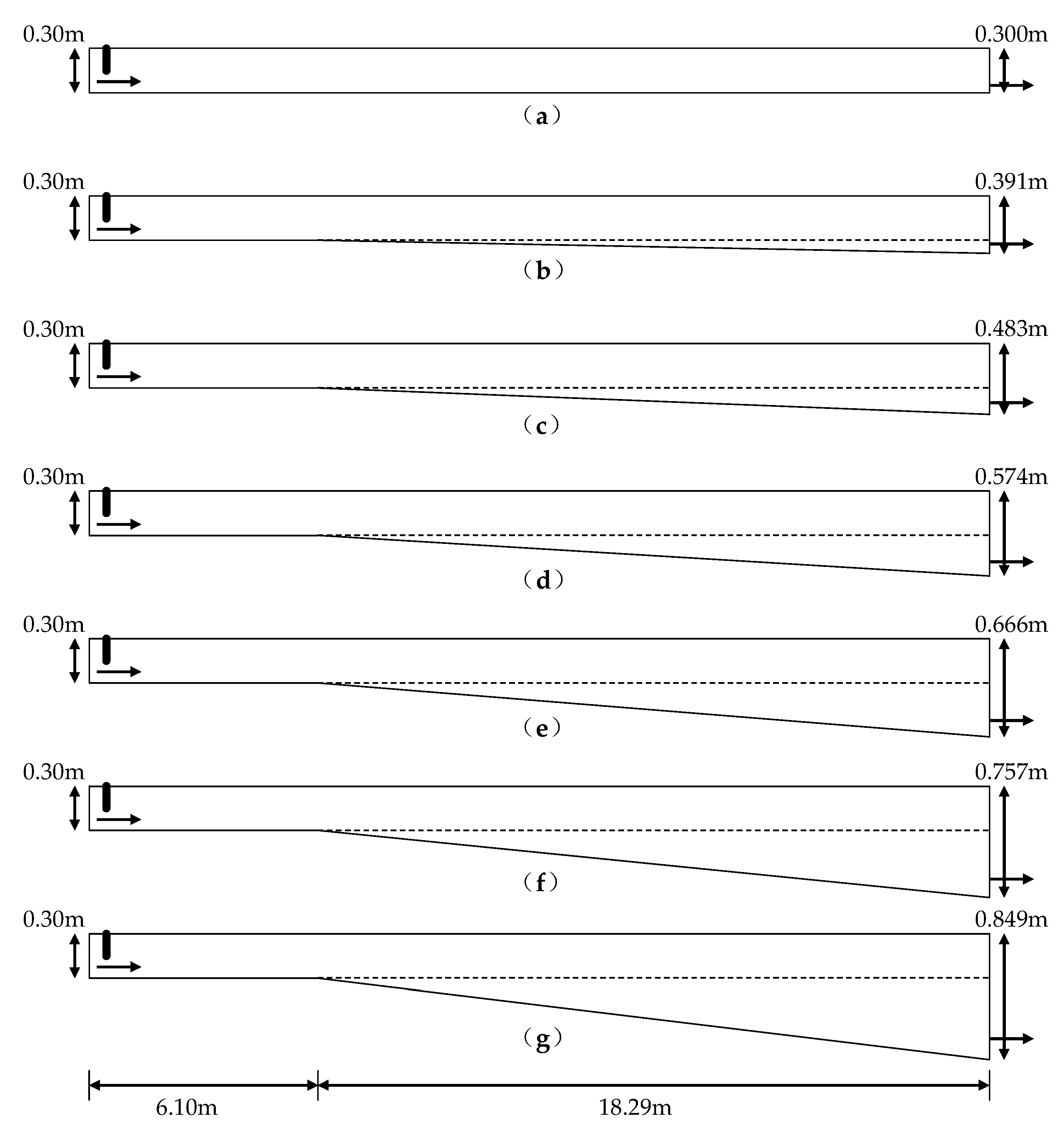
When the bottom slope of a reservoir is zero, which means that the reservoir bed is flat, the σ-coordinate system model is nearly equal to the z-coordinate system model. This indicates that the bottom slope has influence on the simulation results of the two models [30,31]. Seven simulation conditions for the bottom slope from 0‰ to 30‰ are discussed. Since the bottom slope is different, the depth of the downstream section is also different. The location of the outlet hole can be determined by the ratio of the height of the outlet to the depth of the downstream section from the original experimental flume investigated by Johnson [21]. The simulation conditions with different bottom slopes are shown in Table 4, and sketches of different reservoir models are displayed in Figure 3.
3. Results
3.1. Comparison of the σ-Coordinate System and the z-Coordinate System Model
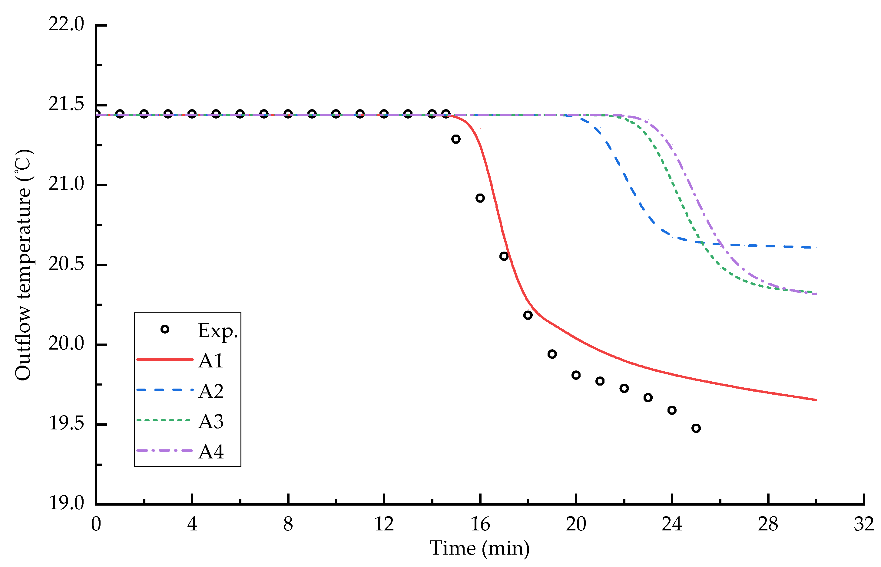
The time variation of the outlet water temperature under different vertical coordinate models is shown in Figure 4, compared to the observed data obtained from Johnson’s experiment [21]. It can be seen that the arrival time of cold water at the outlet for conditions A1 and A2 is 15 and 22 min, respectively. For conditions A3 and A4, the arrival time of cold water at the outlet is around 24 min, which is 9 min later than the observed data. In addition, the outlet water temperature at the end time for conditions A2, A3, and A4 is still much greater than the observed data. The vertical distribution of flow velocity at position 11.43 m from upstream at 11 min under different simulation conditions is shown in Figure 5. According to Figure 5, the thickness of the underflow for conditions A1 and A2 is 0.14 and 0.20 m, respectively, and the thickness of the underflow for conditions A3 and A4 is around 0.23 m, which is nearly twice as high as the observed data. Moreover, the reverse velocity of the upper layer for conditions A2, A3, and A4 is greater than the observed data, which indicates that vertical numerical mixing in conditions A2, A3, and A4 would cause changes in the velocity profile and decrease the velocity of the underflow.
For Figure 4 and Figure 5, it can be concluded that the σ-coordinate system model (condition A1) can accurately simulate the formation process of the density underflow in the GRH flume, and the simulation result of the z-coordinate system model (condition A3) deviates from the observed data. Since cold water flows into the reservoir along the bed, the isotherms exist along the bed too. Therefore, the σ-grids are relatively parallel with the isotherms, and the simulation result of the σ-coordinate system model is close to the observed data. On the other hand, the z-grids are not parallel with the isotherms, which causes significant numerical errors in the z-coordinate system model due to artificial vertical diffusion. Moreover, the anti-creep correction approach in the σ-coordinate system model (condition A2) cannot reduce but instead increase the numerical errors. This is because the anti-creep correction approach takes the approximation of horizontal diffusive fluxes and baroclinic pressure gradients back to the Cartesian coordinate, which leads to new numerical diffusion in the vertical direction due to non-horizontal isotherms. In addition, the method of remapping of near-bottom layers in the z-coordinate system model (condition A4) has less influence on the outlet water temperature and velocity profile in the GRH flume and only reduces the velocity near the bottom. It can be concluded that the anti-creep approach is not suitable when the truncation error of the horizontal baroclinic gradient force is not significant, and the improvement achieved by the remapping of near-bottom layers is not obvious.
3.2. Effect of Grid Resolution on the z-Coordinate System Model
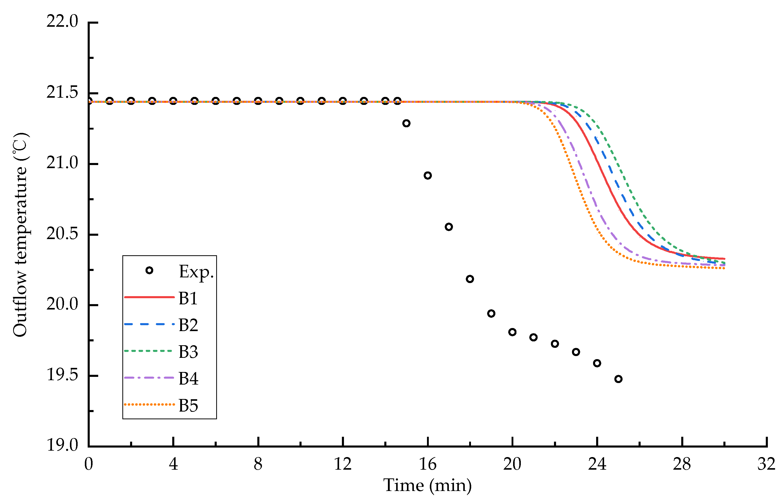
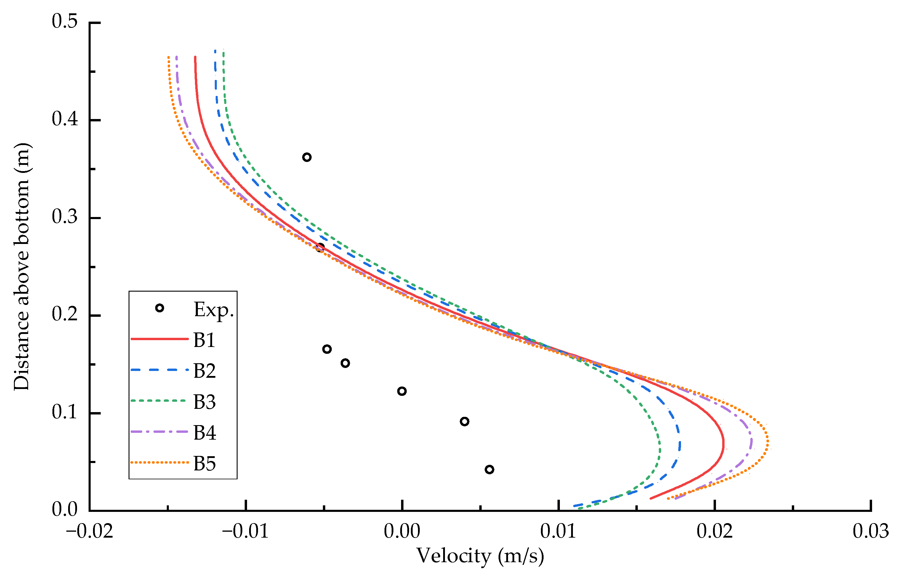
The time variation of the outlet water temperature in the z-coordinate system model with different grid resolutions is shown in Figure 6. It can be seen that the arrival time of cold water at the outlet is slightly delayed with the increase in the vertical grid number (conditions B2~B3), and the arrival time of cold water at the outlet is advanced with the increase in the horizontal grid number (conditions B4~B5). Furthermore, the outlet temperature at the end time of different grid resolutions is nearly the same. The velocity profile at position 11.43 m from upstream at 11 min in the z-coordinate system model with different grid resolutions is shown in Figure 7. According to Figure 7, the velocity of the underflow decreases with the increase in the vertical grid number (conditions B2~B3) and the velocity of the underflow increases with the increase in the horizontal grid number (conditions B4~B5). Moreover, the thickness of the underflow is almost unchanged with different grid resolutions.
For Figure 6 and Figure 7, it can be seen that increasing the vertical grid number is not an effective method to reduce the numerical errors, increasing the horizontal grid number can reduce the deviation between the simulation results of the z-coordinate system model and the observed data. However, the numerical errors caused by the z-coordinate system model are still large after increasing the grid resolution of the cold-water underflow model. It can be concluded that the grid resolution is important to accurately simulate the cold-water underflow in the reservoir, but it is not the main cause of the numerical errors in the z-coordinate system model.
3.3. Effect of Bottom Slope on Simulation Accuracy
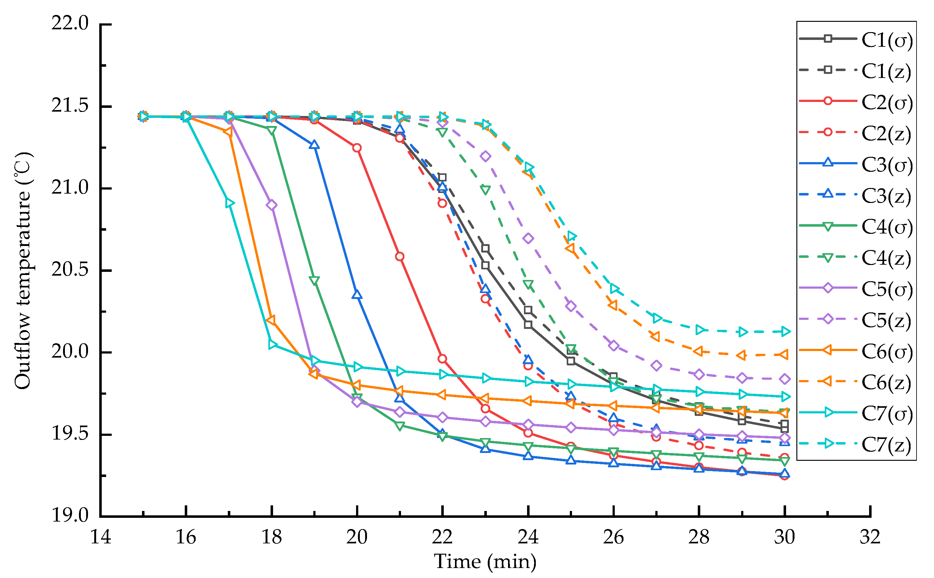
The time variation of the outlet water temperature for both the σ-coordinate system model and the z-coordinate system model with different bottom slopes is shown in Figure 8. According to Figure 8, the characteristics of the two models with different bottom slopes can be summarized as follows:
- When the bottom slope is the same, the outlet water temperature of the σ-coordinate system model is always lower than that of the z-coordinate system model. This means that the z-coordinate system model causes more vertical diffusion and leads to a higher water temperature of the outlet;
- In the σ-coordinate system model, with the increase in the bottom slope, the arrival time of cold water at the outlet is gradually advanced. This suggests that the larger the bottom slope of a reservoir, the higher the velocity of the cold-water underflow. When the bottom slope is more than 10‰ (conditions C4~C7), the outlet water temperature at the end time increases with the increasing bottom slope. This can be explained by the larger bottom slope, which contains more static water with a temperature of 21.44 °C. Compared to a large amount of initial hot water, the cold-water underflow is relatively small, which means that the outlet water temperature is more difficult to decrease;
- In the z-coordinate system model, for condition C2, as the bottom slope increases, the arrival time of cold water at the outlet is advanced; for condition C3, the simulation result is similar to condition C2; for conditions C4~C7, the arrival time of cold water at the outlet is gradually delayed with the increasing bottom slope. This suggests that when the bottom slope is more than 10‰ (conditions C4~C7), the simulation result of the z-coordinate system model may be incorrect;
- Since the σ-coordinate system model can simulate the formation process of cold-water underflow in the reservoir accurately, the simulation result of the σ-coordinate system model can be regarded as a reference to study the effect of bottom slopes on the simulation accuracy of the z-coordinate system model. As shown in Figure 8, when the bottom slope increases, the simulation deviation between the σ-coordinate system model and the z-coordinate system model also increases, which means that the numerical errors caused by the z-coordinate system model continue to increase. It can be concluded that the simulation accuracy of the z-coordinate system model decreases with the increasing bottom slope.
4. Discussion
When simulating cold-water underflow in the reservoir, it is found that the σ-coordinate system model has higher simulation accuracy than the z-coordinate system model. This is because the σ-grid lines are parallel with the flow direction of the cold-water underflow, and the truncation errors of the horizontal baroclinic gradient force caused by the σ-coordinate system model are not significant. The z-grid lines are horizontal and not parallel with the flow direction of the cold-water underflow. The numerical errors caused by artificial vertical diffusion are significant, and the numerical errors due to the staircase representation of the z-coordinate system model cannot be ignored. This indicates that the simulation accuracy of the reservoir water temperature model mainly depends on the relationship between the vertical coordinate grids and the flow direction. For cold water flowing into the reservoir, the flow direction is always along the bottom of the reservoir; therefore, the relationship between the vertical coordinate grids and the bottom slope should be taken into consideration. According to Figure 3 and Figure 8, when the bottom slope also increases, the angle between the z-grid lines and the bottom boundary increases, as do the numerical errors of the z-coordinate system model. There may be a critical value of the bottom slope at which the numerical errors of the z-coordinate system model can be acceptable.
The F-test (joint hypotheses test) is usually used to compare the population variance of two different methods. As the cold-water underflow simulations of the σ-coordinate system model and the z-coordinate system model are two sets of independent data, the F-test can be helpful to determine whether the population variance of the two models is the same or not. When the F value is less than its critical value, it is considered that the population variance of the z-coordinate system model is equal to that of the σ-coordinate system model. The results of the F-test for different simulation conditions are listed in Table 5.
According to Table 5, when the bottom slope is more than 15‰ (conditions C1~C4), the F value is less than the critical value, which means that the simulation result of the z-coordinate system model is acceptable; when the bottom slope is more than 20‰ (conditions C5~C7), the F value is more than the F critical value, which means that the simulation result of the z-coordinate system model is not credible. Therefore, there may be a critical value of the bottom slope between 15‰ and 20‰. Through the F-test for additional simulation conditions with different bottom slopes, it is found that the critical value of the bottom slope is around 18‰. This indicates that when the bottom slope is less than 18‰, the z-coordinate system model is capable of simulating cold water flowing into the reservoir; when the bottom slope is more than 18‰, the z-coordinate system model would cause significant artificial vertical diffusion and artificial flow.
Generally, when selecting the vertical coordinate system, the vertical grid lines should be parallel with the main flow direction in order to avoid artificial vertical diffusion. For a steady-state temperature stratified reservoir, the isotherms tend to be horizontal, as does the flow direction. It is preferable to choose a z-coordinate system model to simulate the water temperature stratification flow. The error caused by the staircase representation of boundaries in the z-coordinate system model can be minimized by increasing the horizontal and vertical grid resolutions, especially the horizontal grid numbers. For cold water flowing into the reservoir, the isotherms are affected by the cold-water underflow and are not horizontal anymore. The σ-coordinate system model is recommended to simulate cold-water underflow in reservoirs. In addition, when the bottom slope is less than 18‰, the z-coordinate system model can also be adopted.
5. Conclusions
For the simulation of cold-water underflow in a reservoir, the characteristics of different vertical coordinate systems were studied with the Delft3D software. The main conclusions are as follows:
- When simulating cold water flowing into a reservoir, the σ-coordinate system model has high simulation accuracy and is not affected by the truncation errors of the horizontal baroclinic gradient force. In contrast, the z-coordinate system model is inaccurate due to artificial vertical diffusion;
- The numerical errors in the z-coordinate system cold-water underflow reservoir model mainly consist of the following two parts: one is caused by the staircase representation of the bottom boundary, and one is caused by artificial vertical diffusion as the vertical grid lines are not parallel with the flow direction;
- To reduce the numerical error caused by the staircase representation of boundaries in the z-coordinate system model, the methods of remapping of near-bottom layers and increasing the vertical grid resolution have little influence on the simulation results. However, the method of increasing the horizontal grid resolution can decrease this numerical error, although there is still a large deviation from the observed data;
- To reduce artificial vertical diffusion in the z-coordinate system cold-water underflow reservoir model, the vertical grid lines should be parallel with the flow direction. The F-test shows that when the bottom slope is less than 18‰, the z-coordinate system model can simulate cold water flowing into a reservoir accurately.
Author Contributions
Conceptualization and methodology, Z.H.; software, validation, data curation, and writing—original draft preparation, Y.L. (Yun Lang); writing—review and editing, Y.L. (Yafei Li) and L.H.; supervision, R.H. The authors have read and agreed to the published version of the manuscript. All authors have read and agreed to the published version of the manuscript.
Funding
This research was funded by the Scientific and Technological Innovation Project of Colleges and Universities in Shanxi Province, 2019L0223; Shanxi Province Water Conservancy Science and Technology Research and Extension Projects, 2022GM017; Research Project Supported by Shanxi Scholarship Council of China, 2021-051; Shanxi Basic Research Program, 202103021223079.
Institutional Review Board Statement
Not applicable.
Informed Consent Statement
Not applicable.
Data Availability Statement
The data presented in this study are available upon request from the corresponding author.
Acknowledgments
We thank the reviewers for their useful comments and suggestions.
Conflicts of Interest
The authors declare no conflict of interest.
References
- Yang, Z.; Liu, D.; Ji, D.; Xiao, S. Influence of the Impounding Process of the Three Gorges Reservoir up to Water Level 172.5 M on Water Eutrophication in the Xiangxi Bay. Sci. China Technol. Sci. 2010, 53, 1114–1125. [Google Scholar] [CrossRef]
- Fu, B.; Wu, B.; Lue, Y.; Xu, Z.; Cao, J.; Niu, D.; Yang, G.; Zhou, Y. Three Gorges Project: Efforts and Challenges for the Environment. Prog. Phys. Geogr. 2010, 34, 741–754. [Google Scholar] [CrossRef]
- Xu, X.; Tan, Y.; Yang, G. Environmental Impact Assessments of the Three Gorges Project in China: Issues and Interventions. Earth-Sci. Rev. 2013, 124, 115–125. [Google Scholar] [CrossRef]
- Gao, Q.; He, G.; Fang, H.; Bai, S.; Huang, L. Numerical Simulation of Water Age and Its Potential Effects on the Water Quality in Xiangxi Bay of Three Gorges Reservoir. J. Hydrol. 2018, 566, 484–499. [Google Scholar] [CrossRef]
- Zhang, M.; Niu, Z.; Cai, Q.; Xu, Y.; Qu, X. Effect of Water Column Stability on Surface Chlorophyll and Time Lags Under Different Nutrient Backgrounds in a Deep Reservoir. Water 2019, 11, 1504. [Google Scholar] [CrossRef]
- Zhang, L.; Xia, Z.; Zhou, C.; Fu, L.; Yu, J.; Taylor, W.D.; Hamilton, P.B.; Cappellen, P.V.; Ji, D.; Liu, D. Unique Surface Density Layers Promote Formation of Harmful Algal Blooms in the Pengxi River, Three Gorges Reservoir. Freshw. Sci. 2020, 39, 722–734. [Google Scholar] [CrossRef]
- Li, Y.; Sun, J.; Lin, B.; Liu, Z. Thermal-hydrodynamic Circulations and Water Fluxes in a Tributary Bay of the Three Gorges Reservoir. J. Hydrol. 2020, 585, 124319. [Google Scholar] [CrossRef]
- Li, P.; Yao, Y.; Lian, J.; Ma, C. Effect of Thermal Stratified Flow on Algal Blooms in a Tributary Bay of the Three Gorges Reservoir. J. Hydrol. 2021, 601, 126648. [Google Scholar] [CrossRef]
- Liu, L.; Liu, D.; Johnson, D.M.; Yi, Z.; Huang, Y. Effects of Vertical Mixing on Phytoplankton Blooms in Xiangxi Bay of Three Gorges Reservoir: Implications for Management. Water Res. 2012, 46, 2121–2130. [Google Scholar] [CrossRef]
- Holbach, A.; Norra, S.; Wang, L.; Yijun, Y.; Hu, W.; Zheng, B.; Bi, Y. Three Gorges Reservoir: Density Pump Amplification of Pollutant Transport into Tributaries. Environ. Sci. Technol. 2014, 48, 7798–7806. [Google Scholar] [CrossRef]
- Zhao, Y.; Zheng, B.; Wang, L.; Qin, Y.; Li, H.; Cao, W. Characterization of Mixing Processes in the Confluence Zone Between the Three Gorges Reservoir Mainstream and the Daning River Using Stable Isotope Analysis. Environ. Sci. Technol. 2016, 50, 9907–9914. [Google Scholar] [CrossRef]
- Yang, Z.; Cheng, B.; Xu, Y.; Liu, D.; Ma, J.; Ji, D. Stable Isotopes in Water Indicate Sources of Nutrients that Drive Algal Blooms in the Tributary Bay of a Subtropical Reservoir. Sci. Total Environ. 2018, 634, 205–213. [Google Scholar] [CrossRef]
- Cheng, Y.; Mu, Z.; Wang, H.; Zhao, F.; Li, Y.; Lin, L. Water Residence Time in a Typical Tributary Bay of the Three Gorges Reservoir. Water 2019, 11, 1585. [Google Scholar] [CrossRef]
- Song, Y.; Shen, L.; Zhang, L.; Li, J.; Chen, M. Study of a Hydrodynamic Threshold System for Controlling Dinoflagellate Blooms in Reservoirs. Environ. Pollut. 2021, 278, 116822. [Google Scholar] [CrossRef]
- Cornelissen, S. Numerical Modelling of Stratified Flows: Comparison of the Sigma and Z Coordinate Systems; Tu Delft: Delft, The Netherlands, 2004. [Google Scholar]
- Haney, R.L. On the Pressure Gradient Force Over Steep Topography in Sigma Coordinate Ocean Models. J. Phys. Oceanogr. 1991, 21, 610–619. [Google Scholar] [CrossRef]
- Mellor, G.L.; Ezer, T.; Oey, L. The Pressure Gradient Conundrum of Sigma Coordinate Ocean Models. J. Atmos. Ocean. Technol. 1994, 11, 1126–1134. [Google Scholar] [CrossRef]
- Zamani, B.; Koch, M. Comparison between Two Hydrodynamic Models in Simulating Physical Processes of a Reservoir with Complex Morphology: Maroon Reservoir. Water 2020, 12, 814. [Google Scholar] [CrossRef]
- Stelling, G.S.; Van kester, J.A.T.M. On the Approximation of Horizontal Gradients in Sigma Co-ordinates for Bathymetry with Steep Bottom Slopes. Int. J. Numer. Methods Fluids 1994, 18, 915–935. [Google Scholar] [CrossRef]
- Platzek, F.; Stelling, G.; Jankowski, J.; Patzwahl, R. On the Representation of Bottom Shear Stress in Z-layer Models. In Proceedings of the 10th International Conference on Hydroinformatics: Hic 2012, Hamburg, Germany, 14–18 July 2012. [Google Scholar]
- Johnson, B.H. A Review of Numerical Reservoir Hydrodynamic Modeling: Us Army Engineer Waterways Experiment Station. 1981. Available online: https://apps.dtic.mil/sti/pdfs/ADA097823.pdf (accessed on 1 February 1981).
- Sarker, S. Essence of Mike 21C (FDM Numerical Scheme): Application on the River Morphology of Bangladesh. Open J. Model. Simul. 2022, 10, 88–117. [Google Scholar] [CrossRef]
- Sarker, S. A Short Review on Computational Hydraulics in the Context of Water Resources Engineering. Open J. Model. Simul. 2021, 10, 1–31. [Google Scholar] [CrossRef]
- Deltares. Delft3d-Flow User Manual; Deltares: Delft, The Netherlands, 2020. [Google Scholar]
- Postma, L.; Stelling, G.; Boon, J. Three-dimensional Water Quality and Hydrodynamic Modelling in Hong Kong, III. Stratification and Water Quality. In Proceedings of the 2nd International Symposium on Environmental Hydraulics, Hong Kong, China, 16–18 December 1998. [Google Scholar]
- Burchard, H.; Baumert, H. On the Performance of a Mixed-layer Model Based on the K-epsilon Closure. J. Geophys. Res.-Ocean. 1995, 100, 8523–8540. [Google Scholar] [CrossRef]
- Winton, M.; Hallberg, R.; Gnanadesikan, A. Simulation of Density-driven Frictional Downslope Flow in Z-coordinate Ocean Models. J. Phys. Oceanogr. 1998, 28, 2163–2174. [Google Scholar] [CrossRef]
- Wang, C.; Huang, B.; Xu, T.; Zhu, D.Z.; Wang, L.; Wang, Y. Numerical Modeling of Energy Dissipation of Internal Solitary Waves Encountering Step Topography. Ocean. Eng. 2022, 259, 111853. [Google Scholar] [CrossRef]
- Xia, M.; Jiang, L. Application of an Unstructured Grid-based Water Quality Model to Chesapeake Bay and Its Adjacent Coastal Ocean. J. Mar. Sci. Eng. 2016, 4, 52. [Google Scholar] [CrossRef]
- Zhang, Y.J.; Ateljevich, E.; Yu, H.; Wu, C.H.; Yu, J.C. A New Vertical Coordinate System for a 3d Unstructured-grid Model. Ocean. Model. 2015, 85, 16–31. [Google Scholar] [CrossRef]
- Chen, C.; Qi, J.; Liu, H.; Beardsley, R.C.; Lin, H.; Cowles, G. A Wet/dry Point Treatment Method of Fvcom, Part I: Stability Experiments. J. Mar. Sci. Eng. 2022, 10, 896. [Google Scholar] [CrossRef]
Figure 1.
Sketch of the generalized reservoir hydrodynamics (GRH) flume. (a) Plan view. (b) Side view.
Figure 1.
Sketch of the generalized reservoir hydrodynamics (GRH) flume. (a) Plan view. (b) Side view.


Figure 2.
Sketch of vertical grids for different simulation conditions. (a) A1, A2. (b) A3. (c) A4.

Figure 3.
Sketch of reservoir models for different bottom slopes. (a) C1. (b) C2. (c) C3. (d) C4. (e) C5. (f) C6. (g) C7.
Figure 3.
Sketch of reservoir models for different bottom slopes. (a) C1. (b) C2. (c) C3. (d) C4. (e) C5. (f) C6. (g) C7.

Figure 4.
Time variation of outlet water temperature under different vertical coordinate models.

Figure 5.
Velocity profile at position 11.43 m from upstream at 11 min for different vertical coordinate models.
Figure 5.
Velocity profile at position 11.43 m from upstream at 11 min for different vertical coordinate models.

Figure 6.
Time variation of outlet water temperature for the z-coordinate system model with different grid resolutions.
Figure 6.
Time variation of outlet water temperature for the z-coordinate system model with different grid resolutions.

Figure 7.
Velocity profile at position 11.43 m from upstream at 11 min of the z-coordinate system model with different grid resolutions.
Figure 7.
Velocity profile at position 11.43 m from upstream at 11 min of the z-coordinate system model with different grid resolutions.

Figure 8.
Comparison of outlet water temperature of the σ-coordinate system and the z-coordinate system models under different bottom slopes conditions.
Figure 8.
Comparison of outlet water temperature of the σ-coordinate system and the z-coordinate system models under different bottom slopes conditions.


Table 1.
Settings of the σ-coordinate system model and the z-coordinate system model.
| Simulation Conditions | Vertical Coordinate System | Horizontal Grid | Vertical Grid Number | |
|---|---|---|---|---|
| Longitudinal Grid Number | Lateral Grid Number | |||
| A1 | σ-coordinate | 80 | 9 | 36 |
| A2 | σ-coordinate (anti-creep) | 80 | 9 | 36 |
| A3 | z-coordinate | 80 | 9 | 36 |
| A4 | z-coordinate (remapping) | 80 | 9 | 36 |
Table 2.
Computational parameters of the three-dimensional numerical reservoir model.
| Simulation Conditions | Time Step (min) | Manning Number (m−1/3s) | Background Horizontal Eddy Viscosity Coefficient (m2/s) | Background Horizontal Eddy Diffusion Coefficient (m2/s) | Turbulence Model |
|---|---|---|---|---|---|
| A1~A4 | 0.01 | 0.009 | 0.01 | 0.01 | k-ε model |
Table 3.
Simulation conditions with different grid resolutions in the z-coordinate system model.
| Simulation Conditions | Vertical Coordinate System | Horizontal Grid | Vertical Grid Number | |
|---|---|---|---|---|
| Longitudinal Grid Number | Lateral Grid Number | |||
| B1 | z-coordinate | 80 | 9 | 36 |
| B2 | z-coordinate | 80 | 9 | 72 |
| B3 | z-coordinate | 80 | 9 | 100 |
| B4 | z-coordinate | 160 | 9 | 36 |
| B5 | z-coordinate | 240 | 9 | 36 |
Table 4.
Simulation conditions of different bottom slopes and different reservoir models.
| Simulation Conditions | C1 | C2 | C3 | C4 | C5 | C6 | C7 |
|---|---|---|---|---|---|---|---|
| Bottom slope | 0‰ | 5‰ | 10‰ | 15‰ | 20‰ | 25‰ | 30‰ |
| Depth of the downstream section (m) | 0.300 | 0.391 | 0.483 | 0.574 | 0.666 | 0.757 | 0.849 |
| Height of the outlet hole (m) | 0.050 | 0.065 | 0.080 | 0.096 | 0.111 | 0.126 | 0.141 |
Table 5.
F-test of two vertical coordinate models with different bottom slopes.
| Simulation Conditions | C1 | C2 | C3 | C4 | C5 | C6 | C7 |
|---|---|---|---|---|---|---|---|
| α | 0.05 | 0.05 | 0.05 | 0.05 | 0.05 | 0.05 | 0.05 |
| F | 1.02 | 1.04 | 1.30 | 1.91 | 3.62 | 19.12 | 43.26 |
| P(F < = f) | 0.48 | 0.48 | 0.33 | 0.14 | 0.02 | 0.00 | 0.00 |
| F critical value | 2.69 | 2.69 | 2.69 | 2.69 | 2.69 | 2.69 | 2.69 |
Publisher’s Note: MDPI stays neutral with regard to jurisdictional claims in published maps and institutional affiliations. |
© 2022 by the authors. Licensee MDPI, Basel, Switzerland. This article is an open access article distributed under the terms and conditions of the Creative Commons Attribution (CC BY) license (https://creativecommons.org/licenses/by/4.0/).
Share and Cite
MDPI and ACS Style
Lang, Y.; Hu, Z.; Hao, R.; Li, Y.; Han, L. Comparative Study on Water Temperature Stratified Flow under Different Vertical Coordinate Systems in Delft3D. Water 2022, 14, 2737. https://doi.org/10.3390/w14172737
AMA Style
Lang Y, Hu Z, Hao R, Li Y, Han L. Comparative Study on Water Temperature Stratified Flow under Different Vertical Coordinate Systems in Delft3D. Water. 2022; 14(17):2737. https://doi.org/10.3390/w14172737
Chicago/Turabian StyleLang, Yun, Zijun Hu, Ruixia Hao, Yafei Li, and Lijuan Han. 2022. "Comparative Study on Water Temperature Stratified Flow under Different Vertical Coordinate Systems in Delft3D" Water 14, no. 17: 2737. https://doi.org/10.3390/w14172737
Note that from the first issue of 2016, this journal uses article numbers instead of page numbers. See further details here.