Different Hydroclimate Modelling Approaches Can Lead to a Large Range of Streamflow Projections under Climate Change: Implications for Water Resources Management

Abstract

The paper compares future streamflow projections for 133 catchments in the Murray–Darling Basin simulated by a hydrological model with future rainfall inputs generated from different methods informed by climate change signals from different global climate models and dynamically downscaled datasets. The results show a large range in future projections of hydrological metrics, mainly because of the uncertainty in rainfall projections within and across the different climate projection datasets. Dynamical downscaling provides simulations at higher spatial resolutions, but projections from different datasets can be very different. The large number of approaches help provide a robust understanding of future hydroclimate conditions, but they can also be confusing. For water resources management, it may be prudent to communicate just a couple of future scenarios for impact assessments with stakeholders and policymakers, particularly when practically all of the projections indicate a drier future in the Basin. The median projection for 2046–2075 relative to 1981–2010 for a high global warming scenario is a 20% decline in streamflow across the Basin. More detailed assessments of the impact and adaptation options could then use all of the available datasets to represent the full modelled range of plausible futures.

1. Introduction

Projections of future water resources and river flow characteristics under climate change are needed to inform planning and adaptation in the water and related sectors. These projections are typically developed by comparing hydrological model simulations for a future time period relative to a historical time period [1]. The future climate inputs are generally informed by the change signal from global or regional climate models. The modelling components and considerations are illustrated in Figure 1.

Global climate models run over coarse spatial scales greater than 100 or 200 km. There are many outputs from global climate models produced by different modelling groups across the world, and they can provide a useful indication of the uncertainty or range in future climate projections. The climate model outputs that are available online generally come from global modelling experiments coinciding with the assessment cycles of the Intergovernmental Panel on Climate Change [2,3].

Regional climate modelling or dynamical downscaling run at much higher resolutions over the region of interest (5 to 20 km), using boundary conditions from global climate models. They potentially add value by modelling atmospheric processes at higher spatial resolutions, as well as resolving surface features, such as mountains, coastlines, and land use [4,5]. However, because of the long computer run times, there are limited outputs from dynamical downscaling, run specifically for the region of interest with boundary conditions from a subset of available host global climate models. In Australia, dynamical downscaling has historically been supported by the different state government agencies to inform local and regional assessments.

The methods used to translate outputs from global and regional climate models to inputs for hydrological modelling generally fall into three categories. The first is the empirical scaling method, where the historical daily rainfall series is scaled by the change signal in the climate model to obtain the future climate series [6,7,8]. The empirical scaling can be done at the annual, seasonal, or daily level. The daily scaling considers changes in the daily rainfall distribution and can reflect the increase in high extreme rainfall intensity under warmer conditions. The empirical scaling method can be relatively easily applied and interpreted. However, the major drawback is that empirical scaling assumes that the future rainfall sequence is the same (but with different daily values) as the historical rainfall sequence.

The second method of using climate model outputs for hydrological modelling is the bias correction method. The bias correction method develops a relationship between the historical daily rainfall from the climate model and the observed catchment rainfall. This relationship is then used to translate the future rainfall simulated by the climate model to future catchment rainfall. Therefore, the bias correction method reflects the changes in all the rainfall characteristics as simulated by the climate model (including the rainfall sequence and multi-year variability). The main limitations of the bias correction method are that (i) the bias that needs to be corrected is often much larger than the change signal itself, (ii) the seasonal and annual change signals after bias correction can be different from the raw change signals, and (iii) it is difficult to robustly bias correct all of the rainfall characteristics (particularly the number of rain days, multi-day accumulations, and spatial correlation) important for runoff generation [9,10,11,12]. Another limitation in the context of hydrological modelling and impact assessment is that the historical bias-corrected rainfall series is no longer the same as the observed series resulting in a different baseline modelled streamflow series to compare the future simulations against.

The third method for hydrological projections is to generate a stochastic future daily rainfall series that reflects the change signal in the various rainfall characteristics [13,14,15,16,17]. This method is appealing because the stochastic data can represent both climate variability and climate change, and the changes in the rainfall characteristics can be informed by climate models or climate change knowledge or simply perturbed for sensitivity or stress testing of the hydrological system. However, there are challenges in running complex models of water resource systems with a large number of stochastic replicates.

The availability of multiple climate projection data sources and hydrological impact modelling approaches, and their evolution, has considerably enhanced scientific knowledge. However, the multitude of products and approaches can also be confusing and add to the challenge of assessing hydrological impacts and developing water resource adaptation options under deep uncertainty.

This paper investigates the projections of future water resources and hydrological metrics modelled by a hydrological model, using future rainfall inputs developed from different methods, informed by different global and regional climate model products. The focus of the paper is to present the hydrological projections from the different methods and data sources, describe the range of uncertainty within and between methods, and discuss the interpretation and implications for water resources applications. The study was carried out using the extensive datasets available for the Murray–Darling Basin in south-eastern Australia.

The paper is organised as follows. Following this Introduction, Section 2 describes the study region, data, and modelling methods. Section 3 presents the modelling results, followed by a discussion of the results and their implications for water resources management in Section 4. Section 5 then summarises the conclusions from this modelling study.

2. Data and Modelling Methods

2.1. Study Region

The study region is the Murray–Darling Basin (MDB) in south-eastern Australia (Figure 2). The MDB supports about half of Australia’s irrigated agriculture, is home to more than two million people, and has extensive water-related environmental assets [18]. Streamflow in the MDB is highly variable, with almost twice the inter-annual variability of rivers in similar climate regions elsewhere in the world [19,20]. The 1997–2009 Millennium drought and the decline in cool season rainfall have significantly impacted people, agriculture, and water ecosystems that depend on the water resources in the Basin [21,22,23]. There have been significant and continuing water reforms in the MDB, particularly to rebalance water use between competing uses and to better cope with long and severe droughts [24]. Hydroclimate projections also indicate that the MDB will be hotter and drier in the future [25] because of changes in the general atmospheric circulation under a warmer climate pushing the cool season storm tracks further south [26,27,28].

2.2. Observed Climate and Streamflow Data

The modelling was carried out for 133 catchments (Figure 2). These are largely unimpaired catchments (with no significant diversions, irrigation, or storage), and are therefore located in the upland areas, with better spatial coverage in the high runoff areas in the south-eastern part of the Basin. The catchment areas range from 120 to 2600 km² (10th to 90th percentile range). These 133 catchments were selected by the Australian Bureau of Meteorology as hydrologic reference stations, defined as gauging stations with relatively high quality, long, and continuous streamflow data [29]. The streamflow data were obtained from the Bureau of Meteorology website (http://www.bom.gov.au/water/hrs/ (accessed on 15 March 2021)).

The source of the observed climate data is the 5 km-gridded daily climate dataset from the Bureau of Meteorology (Australian Gridded Climate Data; [30,31]). The catchment-average daily rainfall data were obtained by averaging the gridded rainfall data for all the grid cells within the catchment. The daily areal potential evapotranspiration (PET) was estimated using Morton’s wet environment evapotranspiration formulation [32,33]. Therefore, for each catchment, a single time series of daily rainfall, PET, and streamflow, from 1981 to 2020, was used for the modelling.

2.3. Rainfall-Runoff Modelling

Daily streamflow was modelled using the GR4J lumped conceptual daily rainfall-runoff model [34]. Daily rainfall and PET were inputs into the model, and the model simulates daily streamflow. The GR4J model was calibrated to best reproduce the daily observed streamflow, by maximising the NSE-Bias (Nash–Sutcliffe efficiency and bias) objective function [35], which reflects a good simulation of daily streamflow with little overall bias over the modelling period. The calibrations were satisfactory in practically all the catchments (daily NSE was greater than 0.6 in more than 80% of the catchments, and overall bias was less than 10% in 85% of the catchments) for the purpose of the modelling experiments here.

The same optimised values of the four parameters from the GR4J model calibrations were used to model the historical (1981–2010) and future streamflow (2046–2075, see below). This is a potential limitation as the model was extrapolated to simulate a future under warmer conditions, higher atmospheric CO₂ concentration, and changes in dominant hydrological processes in longer dry spells projected for the MDB [22,36,37]. Understanding and modelling hydrological non-stationarity is a significant challenge and is the subject of considerable ongoing research, particularly in this region [38,39,40]. The influence of hydrological non-stationarity is not considered here; however, it should not affect the conclusions from this study, which is focussing on the evaluation of different sources of climate projections and climate inputs on streamflow projections.

2.4. Future Rainfall Projections from GCMs and RCMs

The climate projections were sourced from four datasets or products. The first dataset was the 42 global climate models (GCMs) from the CMIP5 (Coupled Model Intercomparison Project) database, coinciding with the Intergovernmental Panel on Climate Change Fifth Assessment Report (IPCC AR5). These GCMs have also been used to develop CMIP5-based climate projections for natural resource management regions across continental Australia [41]. The CMIP6 database is also now available with model outputs still being added, and [42] provided an early comparison of climate projections for Australia from CMIP5 models and CMIP6 models available then. Downscaled CMIP6 datasets for Australia are also being currently developed.

The other three climate projection datasets were from dynamical downscaling, supported by the Victoria, New South Wales, and Queensland state governments (Figure 2). One of the products was VCP19 (Victorian Climate Projections 2019) [43], with 5 km daily rainfall downscaled using the CCAM (Conformal Cubic Atmospheric Model) [44] dynamical downscaling model, with boundary conditions provided by six host CMIP5 GCMs. Unlike most regional climate models that use a limited area approach (see next paragraph), CCAM is a variable resolution global model with high spatial resolution over the region of interest progressively expanding to lower spatial resolution further away. This VCP19 CCAM dataset is only available for Victoria. There is another CCAM dataset from the same modelling group at 12 km of resolution that covers the whole MDB, with boundary conditions provided by five host CMIP5 GCMs. Both datasets were used here, and they are denoted as V-CCAM-A and V-CCAM-B, respectively. Note that the V-CCAM-A simulations used a sea surface temperature (SST) bias correction method before nesting within the host GCM [45] whereas V-CCAM-B relied on spectral nudging with the host GCM [46].

Another dynamically downscaled dataset comes from two generations of NARCliM (NSW/ACT Regional Climate Modelling) [47,48], with 10 km daily rainfall downscaled using the WRF (Weather Research and Forecasting) regional climate model [49]. Datasets are available from downscaling using boundary conditions from three host CMIP5 GCMs (NARCliM1.5) and four host CMIP3 GCMs (NARCliM1.0). Both datasets were used here, and they are denoted as N-WRF-A and N-WRF-B, respectively. The modelling experiments with N-WRF-A were carried out here for all the catchments in the MDB and the modelling experiments with N-WRF-B were carried out only for catchments in Victoria. The WRF modelling also experimented with several physics schemes, and for the purpose of the modelling here, outputs from the best physics scheme (R2) as reported in [50] were used here. In total, three CMIP5-driven R2 simulations in NARCliM1.5 and four CMIP3-driven R2 simulations in NARCliM1.0 were used in this study.

The third dynamically downscaled product comes from Queensland, with 10 km daily rainfall downscaled using CCAM, with boundary conditions provided by 12 host CMIP5 GCMs. This dataset covers the whole of Australia and is denoted as Q-CCAM. The dynamical downscaling was performed following the approach in [45] where monthly sea surface temperatures from GCMs were bias-corrected for mean and variance and used to force CCAM [51,52,53,54]. In addition, CMIP5 radiative forcing, such as greenhouse gases, aerosols, ozone change, and solar variability, were also used. These simulations have a much larger ensemble size than the previous CCAM simulations and consist of three CCAM simulations with interactive ocean models and nine CCAM simulations without interactive ocean models.

The hydrological modelling here compares daily streamflow simulations for a future period in 2046–2075 relative to the 1981–2010 historical period. Simulations for RCP8.5, which represents the highest representative greenhouse gas concentration pathway in CMIP5, were used. For context, this reflects a global average warming of about 2 °C by ~2060 relative to 1995 [2]. (Note that the N-WRF-B simulations come from SRES A2 defined for CMIP3 GCMs, which is comparable to RCP8.5 in the CMIP5 GCMs).

2.5. Generating Future Daily Rainfall Series for Hydrological Impact Modelling

The seasonal and daily empirical scaling methods denoted as SS and DS, respectively, were used to generate the 2046–2075 daily rainfall series using the climate change signal from all the above climate projection datasets. In the seasonal scaling (SS) method, after scaling the historical daily rainfall by the four seasonal change factors, the daily rainfall series was further rescaled by another factor (generally close to 1.0) to match the annual change signal from the climate model. The daily scaling (DS) method was applied separately to each of the four seasons. The daily rainfall series was then further rescaled twice, first to match the raw change signal from the climate model in each of the four seasons, and then to match the raw annual change signal from the climate model.

The bias correction method, denoted as BC, was also used to generate the 2046–2075 daily rainfall series informed by the three dynamical downscaling products. The quantile-quantile approach was applied to each season separately, mapping the downscaled daily rainfall to the observed catchment daily rainfall cumulative density function, such that the downscaled daily rainfall amount was replaced with the observed daily rainfall amount for the corresponding percentile [9,55]. The seasonal and annual change signals after bias correction can be quite different from the change signals in the raw downscaled data, more so than in the above empirical scaling methods. However, unlike in the empirical scaling methods, the bias-corrected daily rainfall series was not rescaled to match the seasonal and annual change signals in the raw downscaled data as this would have negated the purpose of the approach to reflect changes in the different rainfall characteristics as simulated by the dynamical downscaling.

Mean monthly PET values (i.e., 12 values, one for each month, the same value was used for all the days in the month) were used as input to model the future period. These were obtained by scaling the historical monthly PET by the ratio of the future PET versus historical PET estimated from the climate simulations (mainly temperature and relative humidity) from the GCMs. For the dynamical downscaling products, the changes in PET from the host GCMs providing the boundary conditions were used.

The climate projection products and the approaches used to generate future daily rainfall series, as described above, are summarised in

Table 1. Climate projection products and methods used to generate future daily rainfall series.

	Climate Projections Product	Number of Datasets	Methods Used to Generate Future Rainfall Series *
GCM	42 CMIP5 GCMs 100–300 km resolution, all MDB	42	SS, DS
V-CCAM-A	VCP19 CCAM 6 host CMIP5 GCMs, 5 km resolution, only Victoria	6	SS, DS, BC
V-CCAM-B	ESCI CCAM 5 host CMIP5 GCMs, 12 km resolution, all MDB	5	SS, DS, BC
Q-CCAM	Queensland CCAM 12 host CMIP5 GCMs, 10 km resolution, all MDB	12	SS, DS, BC
N-WRF-A	NARCliM WRF 3 host CMIP5 GCMs, 10 km resolution, all MDB	3	SS, DS, BC
N-WRF-B	NARCliM WRF 4 host CMIP3 GCMs, 10 km resolution, only Victoria	4	SS, DS, BC

* SS is seasonal scaling, DS is daily scaling, BC is bias correction.

.

3. Results

3.1. Hydrological Characteristics Assessed in the Study

The changes in future mean annual rainfall, and modelled mean annual streamflow, high flow days, and hydrological drought are presented here. The changes in the hydrological characteristics were calculated by comparing the modelled future (2046–2075) and historical (1981–2010) daily streamflow series. The high flow days are defined here as the number of days above the 99th percentile daily streamflow threshold in the historical period (Q₉₉) (occurring on average 3.6 days per year), reflecting high flow events important for environmental outcomes. For example, a value (change) of −2 indicates that there are 1.6 days on average per year above the 99th percentile daily streamflow in the future simulation compared to 3.6 days in the historical simulation. The hydrological drought is defined here as the number of 1-in-10-year droughts indicated by the non-overlapping 3-year total streamflow (occurring three times in the 30-year historical period). The hydrological drought indicates long periods with low streamflow that the system needs to cope with and recover from [23], noting that it is difficult to meaningfully define this with the relatively short sample of 30 years of simulations here. For example, a value (change) of 1 indicates that there are 4 non-overlapping 3-year total streamflows in the future simulation that are lower than the threshold in the historical data compared to 3 in the historical simulation.

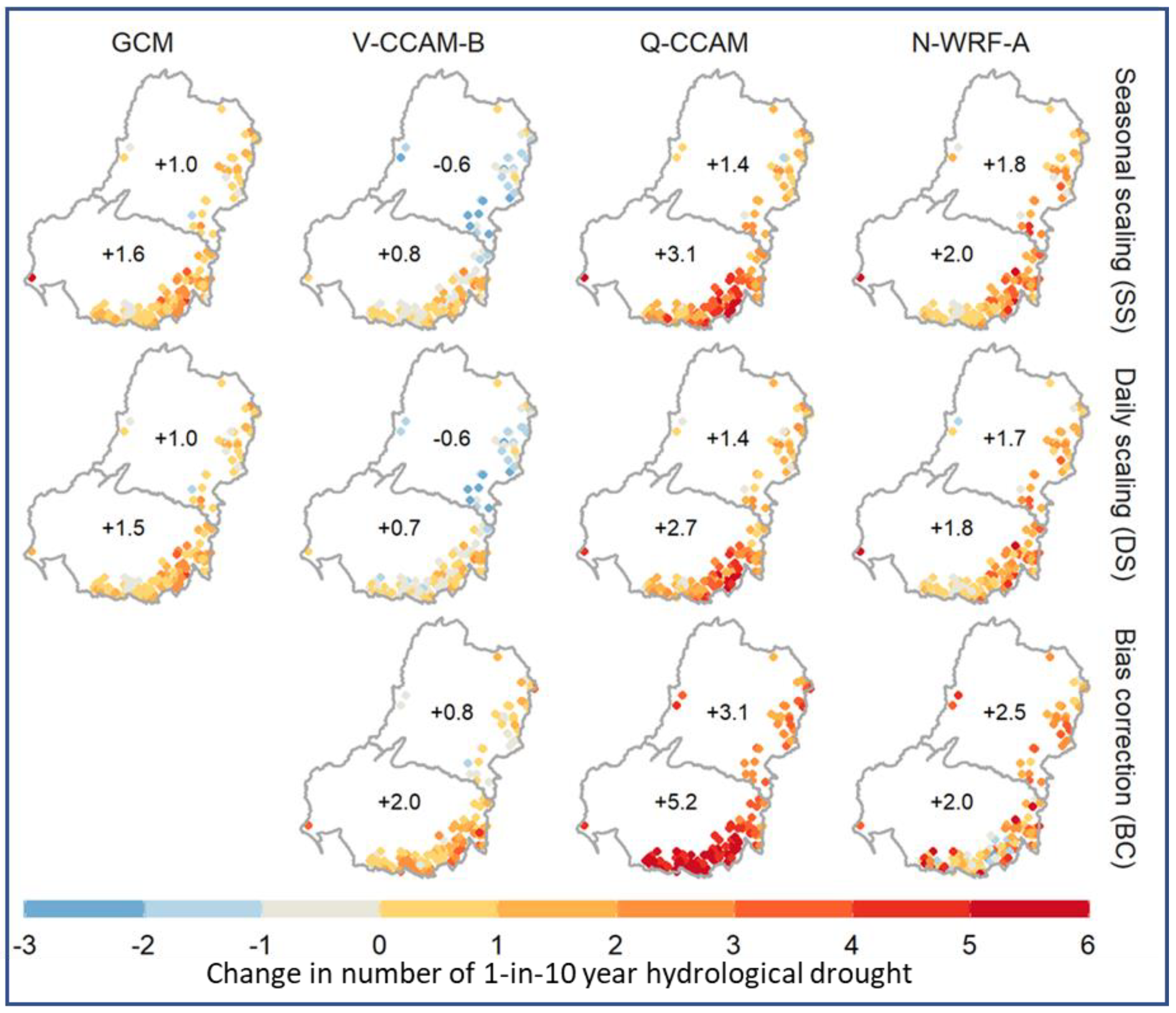
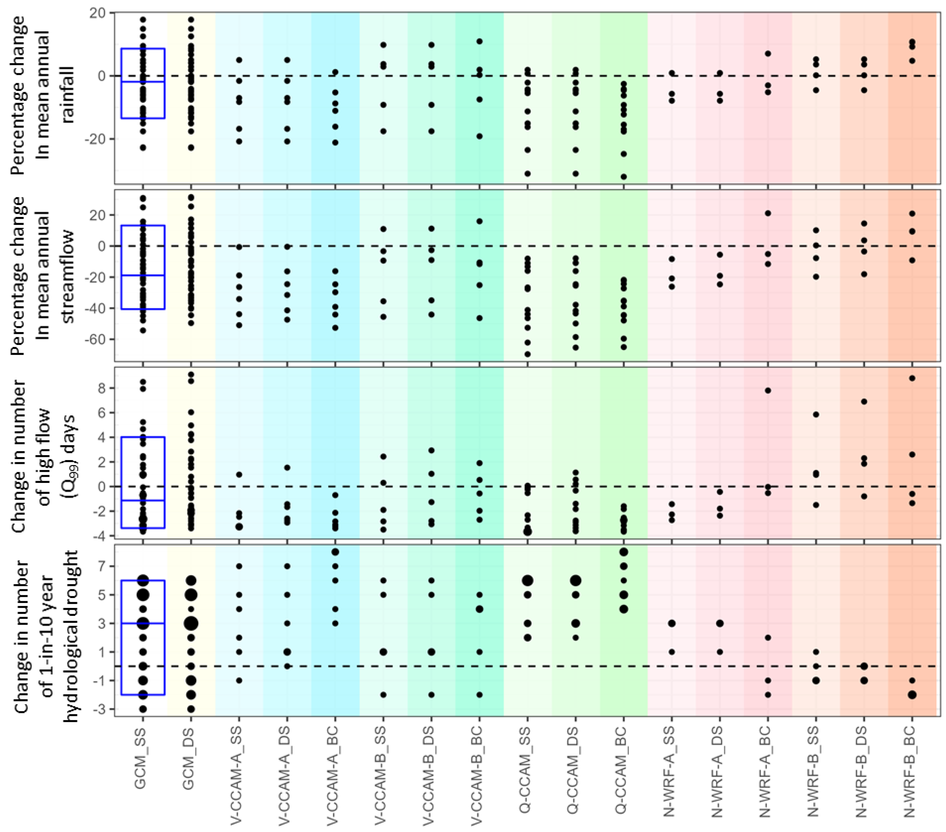
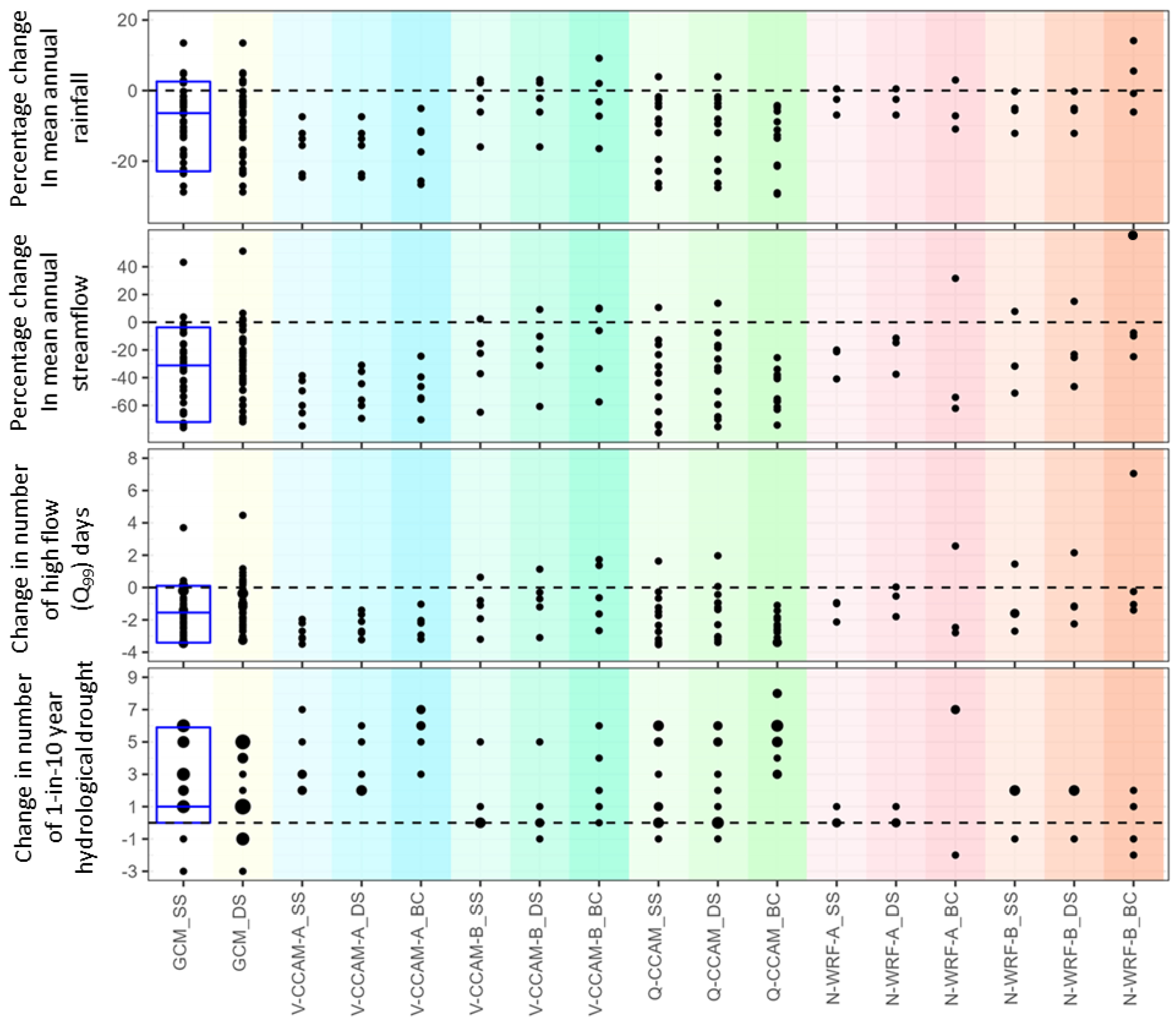
3.2. Median Projected Change in Hydrological Characteristics in the 133 Catchments from Each Climate Projection Data Source and Method Used to Generate Future Daily Rainfall Series

Figure 3, Figure 4 and Figure 5 present the median projected change in the 133 catchments across the MDB, from the range of projections informed by each climate projection product (except V-CCAM-A and N-WRF-B where simulations are available only for Victoria) and the three methods used to generate future daily rainfall series, for the mean annual streamflow, high flow days, and hydrological drought, respectively. The averages of the median projections from all the catchments in the northern MDB (Darling River Basin) and the southern MDB (Murray River Basin) are also shown in the plots.

The results show that the projected percentage decline in future rainfall across the MDB is amplified in the percentage decline in the streamflow (Figure 3) and leads to fewer high flow days (Figure 4) and more frequent hydrological droughts (Figure 5). The climate change impact on the streamflow is greater in the southern MDB. The median projection from the hydrological modelling informed by the climate change signal in the 42 GCMs (for ~2 °C global warming as described in Section 2), and the seasonal scaling method is a 23% decline in the mean annual streamflow averaged across all the catchments in southern MDB and a 19% decline averaged across the catchments in northern MDB (first column in Figure 3).

The median projection for high flow days averaged across all the catchments is 1.5 fewer high flow days in the northern MDB (2.1 days per year with daily streamflow above Q₉₉ in the future period compared to 3.6 in the historical period) and 0.8 fewer high flow days in the southern MDB (2.8 days per year with daily streamflow above Q₉₉ in the future period compared to 3.6 in the historical period (first column of Figure 4). The median projection for hydrological drought is about one to two more 1-in-10-year 3-year non-overlapping low streamflows compared to the historical period (and greater in some catchments), indicating that the hydrological drought that occurs once every 10 years in the historical period will occur once every 6 or 7 years in the future period (first column of Figure 5).

3.3. Range of Future Projections for Rainfall and Hydrological Characteristics within and across the Different Climate Projection Data Sources and Methods Used to Generate Future Daily Rainfall Series for Two Catchments

Figure 6 and Figure 7 present the projected changes in future mean annual rainfall, mean annual streamflow, high flow days, and hydrological drought for two catchments in Victoria, the state where modelling was carried out for all the datasets and methods in Table 1. There is large uncertainty in the modelled projection informed by each climate projection product because of the large uncertainty or range in the future rainfall projection. Figure 6 (first column) indicates that the mean annual rainfall projection across the 42 GCMs for Catchment 401212 ranges from −13% to +8% change (10th to 90th percentile range), and this leads to a modelled change of −40% to +12% in the mean annual streamflow (median of −19%), change of −3 to +4 days above Q₉₉ (median of −1 day), and −2 to +6 more 1-in-10-year hydrological drought (median of 3, or a 1-in-10-year drought in the historical period becoming a 1-in-5-year drought in the future period). Figure 7 (first column) indicates a larger impact in Catchment 415207, with mean annual rainfall changing by −22% to +2%, mean annual streamflow ranging from little change to a decline of up to 70%, high flow days ranging from a small decrease to potentially very few high flows days in the future period, and hydrological drought ranging from a small increase to being much more frequent (1-in-10-year drought occurring up to more than eight times in the future 30-year simulation period compared to three times in the 30-year historical simulation period).

3.4. Seasonal Scaling and Daily Scaling Methods

The mean annual rainfalls from the seasonal scaling and daily scaling methods are the same because after scaling to reflect the change in the future daily rainfall distribution, the daily rainfall is further rescaled to match the seasonal (and then annual) change signal. However, the projected change in the streamflow metrics can be different because daily scaling accounts for the potential increase in the very high daily rainfall that generates high runoff. This is most evident for the high flow days in the southern MDB with the daily scaling method, as expected, simulating more high flow days (larger increase or smaller decrease in future high flow days) than the seasonal scaling method (third row of Figure 6 and Figure 7, and the first two rows of Figure 4). The average of the median projection from all the catchments in the southern MDB is 1.0 fewer high flow days in the future period from the daily scaling method compared to 1.5 fewer high flow days from the seasonal scaling method, with the climate change signal informed by the 42 GCMs, 0.4 fewer high flow days from daily scaling compared to 0.8 fewer high flow days from seasonal scaling when informed by V-CCAM-B, 1.6 fewer high flow days from daily scaling compared to 2.2 fewer high flow days from seasonal scaling when informed by Q-CCAM, and 1.4 fewer high flow days from daily scaling compared to 1.8 fewer high flow days from seasonal scaling when informed by N-WRF-A.

Unlike in the southern MDB, the modelled projected change in high flow days from the daily and seasonal scaling methods for catchments in the northern MDB are similar. The mean annual streamflow from the daily scaling method is also slightly higher than from the seasonal scaling method, but the differences are relatively small as can be seen in the second rows of Figure 6 and Figure 7 and the first two rows of Figure 3 (e.g., the average decline in the mean annual streamflow of 21% across the southern MDB from the daily scaling method compared to 23% from the seasonal scaling method). There is little difference between the hydrological drought simulations from the seasonal and daily scaling methods (the first two rows of Figure 5).

3.5. Projections from GCMs and the Different Dynamical Downscaling Products

The future simulations from V-CCAM-B are considerably wetter (or less dry) than from the 42 GCMs. The median projection from the seasonal scaling method averaged across all the catchments in the southern MDB from V-CCAM-B is 11% lower mean annual streamflow (compared to 23% from the GCMs), 0.8 fewer high flow days (compared to 1.5 in the GCMs), and 0.8 more 1-in-10-year hydrological droughts (compared to 1.6 in the GCMs) (first row of Figure 3, Figure 4 and Figure 5). For the northern MDB, unlike all the other climate projection products, VCCAM-B projects a slightly wetter future (first two of Figure 3, Figure 4 and Figure 5). In contrast to V-CCAM-B, where the projections are wetter than from the GCMs, the V-CCAM-A projections (only available for Victoria) are generally drier than from the GCMs (Figure 6 and Figure 7). It should be noted again that the downscaling experiments are informed by a subset of the 42 GCMs rather than results driven by all 42 GCMs (as can be seen in Figure 6 and Figure 7).

The projected change from N-WRF-A, from the scaling methods, for Catchments 401212 and 415207, is generally within the range of the projected change from the full suite of 42 GCMs (Figure 6 and Figure 7). The median projection from N-WRF-A is slightly drier than from the GCMs for catchments in the southern MDB and considerably drier for catchments in the northern MDB. Averaged across southern MDB, the median projection from the seasonal scaling method for N-WRF-A is 26% lower mean annual streamflow (compared to 23% from the GCMs), 1.8 fewer high flow days (compared to 1.5 in the GCMs), and 2.0 more 1-in-10-year hydrological droughts (compared to 1.6 in the GCMs) (first row of Figure 3, Figure 4 and Figure 5). Averaged across northern MDB, the median projection from the seasonal scaling method for N-WRF-A is 31% lower mean annual streamflow (compared to 19% from the GCMs), 1.4 fewer high flow days (compared to 0.8 in the GCMs), and 1.8 more 1-in-10-year hydrological droughts (compared to 1.0 in the GCMs) (first row of Figure 3, Figure 4 and Figure 5). In contrast, the N-WRF-B projections for Victoria (simulations are only available for Victoria) are wetter than the projections from N-WRF-A and the GCMs, and generally show little change or a slightly wetter future (Figure 6 and Figure 7). Nevertheless, it should be noted that the results for N-WRF-A and N-WRF-B are based on a limited sample size of three and four dynamic downscaled projection datasets respectively.

The projected change from Q-CCAM for the southern MDB is much drier than from the 42 GCMs and is the driest of the climate projection products. Averaged across southern MDB, the median projection from the seasonal scaling method for Q-CCAM is 35% lower mean annual streamflow, 2.2 fewer high flow days (i.e., only 1.6 days per year above Q₉₉ in the future period compared to 3.6 days in the historical period) and 3.1 more 1-in-10-year hydrological droughts (i.e., a 1-in-10-year hydrological drought in the historical period becoming a 1-in-5-year drought in the future period) (first row of Figure 3, Figure 4 and Figure 5). The projected change from Q-CCAM for the northern Basin is also considerably drier than from the 42 GCMs, but slightly less dry than N-WRF-A. Averaged across northern MDB, the median projection from the seasonal scaling method for Q-CCAM is a 27% lower mean annual streamflow (compared to 19% from the GCMs), 1.2 fewer high flow days (compared to 0.8 in the GCMs), and 1.4 more 1-in-10-year hydrological droughts (compared to 1.0 in the GCMs) (first row of Figure 3, Figure 4 and Figure 5).

3.6. Bias Correction Method

The projections from the bias correction method can be very different compared to the seasonal and daily scaling methods. However, there is no consistent indication of drier or wetter simulations in the bias correction compared to the scaling methods. The projections for the southern basin from the bias correction and daily scaling methods are similar for V-CCAM-B, whilst bias correction leads to drier projections with Q-CCAM and wetter (or less dry) projections with N-WRF-A (Figure 3 and Figure 4). For the northern basin, bias correction leads to wetter (or less dry) projections for V-CCAM-B and N-WRF-A, and slightly drier projections for Q-CCAM (Figure 3 and Figure 4).

4. Discussion

4.1. Sources of Climate Projection Data for Hydrological Impact Modelling

The largest uncertainty in the streamflow projection comes from the uncertainty in the future rainfall projection. The uncertainty in the rainfall projection is considerably larger than the differences between hydrological models [56,57,58] and methods used to generate future rainfall series (as seen in the modelling results here). Nevertheless, it should be noted that there are also limitations when extrapolating hydrological models to predict the future [22,36,38], and the differences between hydrological models in predicting some hydrological metrics can also be large particularly low flow characteristics [59,60].

The relatively large number of archived global climate model (GCM) datasets can provide a useful indication of the uncertainty and range in the future rainfall projection. Numerous studies have explored reducing the uncertainty by putting more weight on, or only using, the GCMs that can best simulate the observed climatology. Although some studies show that this can reduce the range in the projections in some regions, the majority of studies show little correlation between the “better” GCMs and future rainfall projections; therefore, using only the better GCMs tends to provide similar projections as using all the available GCMs. The GCMs may also perform differently under different evaluation criteria (e.g., the ability to reproduce observed rainfall over the MDB versus the whole of Australia, the ability to simulate large-scale atmospheric and oceanic indices or drivers of rainfall (such as ENSO), ability to simulate the relationship between large scale drivers and regional rainfall), making the choice of GCMs difficult (selected Australian studies include [41,61,62,63]. Some dynamical downscaling studies select host GCMs that are more independent in their physics schemes used to model the atmospheric, land, and ocean processes, and have shown that downscaling informed by more “independent” GCMs can reduce the uncertainty in the future climate projections [64,65].

The added value of using regional climate models to downscale data from coarse resolution global climate models has been extensively researched [66,67]. For example, [68], through analysing daily precipitation outputs from the EURO-CORDEX and CORDEX-CORE downscaled projection ensembles, showed an overall positive added value from regional climate models for most precipitation metrics, especially for the tail end of the distribution. Reference [4] showed added value from downscaling in areas of complex topography and coastlines, as well as in tropical regions. Regional climate models used for producing climate change projections share with global climate models uncertainties associated with future emission trajectories, internal variability of the climate system, and physical representation of climate processes [69]. The additional uncertainties related to the regional climate models themselves need to be accounted for when evaluating regional projections from downscaling [70].

Dynamical downscaling generally simulates the historical climate better than the GCMs because the physics schemes and parameterisations for the dynamical downscaling are inevitably chosen to best reproduce the historical climatology in the region. For the same reason, the range in the future rainfall projections from a particular dynamical downscaling for a specific region also tends to be smaller than that from the GCMs [71,72,73]. The downscaled rainfall projection, particularly from CCAM, can also be quite different from the rainfall projection of the host GCM (after aggregation to compare at the GCM scale) [43,74].

Compared to GCMs, there are fewer dynamical downscaling datasets because the dynamical downscaling model needs to be developed and parameterised for the region of interest and because of the long computer run times required by much higher resolution modelling. In fact, the dynamical downscaling datasets available for the MDB are plentiful compared to most other parts of the world, because of the importance of the region and because of support from the different states in the MDB, opportunistically providing the datasets for the modelling experiments in this study.

The downscaled projections are influenced by the boundary conditions provided by the host GCMs. The V-CCAM downscaling selected the host GCMs to provide a similar range as the range of projections from all 42 CMIP5 GCMs. It is interesting to note that the same V-CCAM dynamic downscaling can give different results, depending on the downscaling method used, for example, bias correction of sea surface temperature in V-CCAM-A and spectral nudging of sea surface temperature in V-CCAM-B. The two V-CCAM models can therefore be essentially considered as two different downscaling models, with the V-CCAM-A future projections for this region being drier than the V-CCAM-B projections. The host GCMs used for the Q-CCAM downscaling is based on the availability of sea surface temperature and sea ice outputs from the GCMs, and the GCM skill and spread of climate change signal across Australia [51]. It is interesting to note that the Q-CCAM projections are considerably drier than the V-CCAM projections. The four host GCMs used in N-WRF-B are selected based on GCM performance and independence [47,48], and the three host GCMs used in N-WRF-A are selected to represent future scenarios of little change, some drying, and significant drying across the region. The more recent N-WRF-A future projections are hotter and drier than the N-WRF-B projections (Section 3; Figure 6 and Figure 7; [48]).

In summary, the results here show that projections from different downscaling products can be very different, which has also been reported in previous studies [74,75]. Although the differences in the projections can be partly explained by the different host GCMs used, uncertainty related to the experimental setup and physical parameterisation is a significant contributor to the divergence in projected changes in rainfall.

Therefore, although there is a clear value in dynamical downscaling research to understand the processes and evolution of (and changes in) weather dynamics, is difficult to test or know if the future rainfall projections from particular downscaling simulations are better or more reliable or if the projections are better than those from the GCMs.

4.2. Methods Used to Generate Future Rainfall Series for Hydrological Impact Modelling

Various methods have been used to generate future rainfall series for hydrological modelling. Similar to the above discussion about climate projection products, the use of a more complex method does not necessarily lead to more robust projections. Instead, it is important to understand what the method is doing, what rainfall change signal in the climate model simulation it is considering, and how these impact the hydrological modelling and objectives of the modelling study.

The seasonal scaling method is attractive because it is simple to understand and communicate and can be relatively easily applied. The daily scaling method is an advancement of the seasonal scaling method where changes in daily rainfall distribution are also considered. The daily scaling method is potentially advantageous because it can reflect the increase in high extreme rainfall intensity expected under warmer conditions and simulated by most climate models. This is important because a significant amount of runoff is generated during high rainfall events. For example, the modelling results here show that the daily scaling method simulates more high flow days than the seasonal scaling method (reflected as a larger increase or smaller decrease in future high flow days) (Section 3, Figure 4). However, the differences between the methods are relatively small for most other hydrological metrics, for example, the daily scaling method simulates only a slightly higher mean annual streamflow compared to the seasonal scaling method (Figure 3) and both methods give similar projections for hydrological drought (Figure 5). As such, the additional effort and care that must be taken when using the daily scaling method over the seasonal scaling method may not always be necessary. The latter is important and requires looking into the data carefully rather than simply applying a computer algorithm for daily scaling.

For example, early modelling results in this study for a couple of catchments showed increases in the mean annual streamflow despite projected decreases in rainfall. Looking at the data in more detail revealed that some of the dynamical downscaling projected more than a five-time increase in the highest daily rainfall. This potentially unrealistic simulation for only the several highest daily rainfalls in the 30 years of simulation will have minimal effect on the mean annual rainfall, but because all the high daily rainfalls become runoff directly this will result in a significantly higher simulation of mean annual streamflow. Therefore, the realism and causality of these simulations need to be considered and included or modified as appropriate. For the purpose of the modelling here, the daily scaling factor (and likewise in the bias correction method) is constrained to an upper limit of 2.0.

The assumption that the future daily rainfall sequence is the same as the historical daily rainfall sequence is a significant limitation of the seasonal and daily scaling methods. This limitation can be overcome by using daily rainfall simulations from the climate models. However, there is considerable bias in the climate model simulation of rainfall over all the temporal scales. To overcome this, bias correction methods are applied; that is, developing a relationship between the historical daily rainfall from the climate model and the observed catchment rainfall and then using this relationship to translate the future rainfall simulated by the climate model to future catchment rainfall.

The bias correction method is attractive because, in theory, it reflects the changes in all the rainfall characteristics as simulated by the climate model, including rainfall sequence and multi-year variability. However, it is difficult to know what specific rainfall characteristic is being changed and how the characteristic influences streamflow, and whether the climate models have any skill in predicting these. Further, questions can be raised about the realism of the underlying climate modelling when the bias that needs to be corrected is often much larger than the change signal itself [9,76,77]. It is also difficult to robustly bias correct some of the rainfall characteristics, particularly rainfall sequencing, which is important for runoff generation. Bias correction methods are generally statistical in nature and, by explicitly disregarding the modelling of physical processes, can result in the amplification of structural errors and biases in the climate process modelling [11]. A particular example is wet and dry spells, where climate models often produce too many rainfall days (the “drizzle effect”) and this is not corrected by standard bias correction methods [9,78,79]. This probably explains the large variation in the bias correction results and no consistent indication of drier or wetter simulations compared to the empirical scaling methods. There is considerable research attempting to overcome these limitations, and examples include bias correcting rainfall at multiple nested time scales and accounting for daily rainfall correlation structures [80,81,82]. However, there are also many assumptions in these, and their value in hydrological impact modelling requires careful consideration and interpretation as the same apparently positive efforts could also be corrupting the change signals that are important for the specific hydrological application.

In addition, after bias correction, the seasonal and annual change signals are no longer the same as the raw change signals in the climate model [10], and this may require communication, interpretation, and choice depending on the application. For the purpose of the modelling here, the bias-corrected daily rainfall series is used directly rather than rescaled to match the raw seasonal and annual change signals as this would negate the purpose of the bias correction to reflect changes in all the rainfall characteristics as simulated by the climate model. Similar to the daily scaling method, the complex and laborious manipulations in the bias correction also require checking the data carefully, rather than simply applying a computer algorithm for the bias correction, in order to identify potentially unrealistic or erroneous outputs from the data manipulation. Another limitation in the context of hydrological modelling and impact assessment is that the historical bias-corrected rainfall series is no longer the same as the observed series resulting in a different baseline modelled streamflow series to compare the future simulations against. This can be a challenge in communicating the (historical) simulations, particularly in some water resources applications that must use the observed historical streamflow and not a different baseline modelled series.

4.3. Implications for Water Resources Management

The availability of many climate projection products in the MDB (Section 4.1) and the consideration of different methods to generate future rainfall series for hydrological impact modelling (Section 4.2) can provide a fuller and more robust exploration of future hydroclimate and uncertainty in future projections. However, the same availability of many datasets and methods can also be confusing, particularly to catchment and water resources managers, planners, and decision-makers. This is particularly so when different state jurisdictions use different methods and hydroclimate projections whilst water resources planning and adaptation seek to enhance outcomes for the regions as well as the whole MDB.

The many datasets and methods can magnify the perception of deficit in hydroclimate science, and the need to wait for more certainty in the hydroclimate projections before considering climate change in water resources planning [83,84,85,86]. This is unfortunate because, despite their differences, practically all the projection datasets point to a hotter and drier future in the MDB, which will be amplified as a decline in streamflow with more frequent and severe hydrological droughts (Section 3). The national climate projections developed for Australia over the past two decades, generally updated after the release of IPCC assessment reports, have also consistently projected hotter and drier conditions, particularly in the southern MDB [42,87,88].

Although hydroclimate science and modelling will continue to improve, the uncertainty in future projections is likely to remain large because of the challenges in understanding and modelling the complex global and regional atmospheric and land surface processes under current and future climates. However, there is already sufficient knowledge and consistency in the projections to consider and assess adaptation options and scenarios. This is particularly so for engineering applications and water resources management, where uncertainty is acknowledged and formally considered in management and planning through probabilistic and stochastic frameworks. The top-down hydroclimate impact modelling presented in this paper can also be complemented with a bottom-up system approach that “stress-test” the water resources system to characterise and quantify system vulnerability and reliability under different climate inputs [89,90,91]. The top-down hydroclimate projections and bottom-up consideration of system outcomes can then be used to better inform decisions that consider risk versus reward in the different adaptation options (cost of adaptation versus the cost of not adapting fast enough).

Nevertheless, most adaptation considerations start with a top-down impact assessment, and to overcome the confusion and challenges in interpreting the plethora of climate projection datasets and modelling methods, several approaches are proposed here. A useful first step would be to just use a couple of simple future scenarios to assess the potential impact on the different stakeholders and realistic adaptation options and water resources management levers that can reduce the climate change risk. For example, two scenarios could be adopted for the MDB, a median or mid-range scenario (e.g., 20% decline in future water resources as indicated in Figure 3 and 50% more frequent hydrological drought as indicated in Figure 5), and a dry end scenario (e.g., 40% decline in future water resources and twice more frequent hydrological drought). These simple scenarios are easy to communicate to stakeholders, water managers, and policymakers. This will provide a better appreciation of the potential impact, and risk versus reward of the various adaptation options, and are more likely to lead to adaptation actions. In many applications, the use of these scenarios may be sufficient, particularly when all the different datasets and methods indicate the need to adapt to a hotter and drier MDB, but with uncertainty around how much and by when.

It is possible that some adaptation considerations may require a fuller understanding of the uncertainty in the hydroclimate projections. For these, it is probably best to use all the available datasets as presented here (unless they are clearly unrealistic or erroneous) to represent the full range of plausible futures [41,43,92]. At the very least, researchers, stakeholders, and water resources managers should be aware of the different hydroclimate projection datasets and their similarities and differences, and whether the differences matter in the management decisions and outcomes. A better understanding of the different datasets and methods will enable optimum and fit-for-purpose choices based on the science and modelling combined with pragmatic decisions influenced by resources available and the importance and objectives of the modelling study. There are often good reasons to adopt locally developed approaches because of the investment and accumulated learnings from research and modelling and the goodwill that has been established with stakeholders. In the context of the MDB, different approaches may be used for different regions and needs, but with a good understanding of the implications in the context of the range of datasets and methods available.

5. Conclusions

The paper compares future streamflow projections modelled by a hydrological model with future rainfall inputs generated from different methods informed by climate change signals from different global climate models and dynamically downscaled datasets. The large number of archived global climate model datasets is useful in providing an indication of the plausible range of future rainfall. Dynamical downscaling can potentially add value at the local or catchment scale; however, the modelling results here show that future hydroclimate projections from the different dynamical downscaling products can be very different, with some downscaled datasets being wetter and some being drier compared to the global climate models.

The empirical scaling method, which scales the historical rainfall series by the change signal in the climate model, is relatively simple to apply and communicate. Scaling at the daily level, which takes into account more intense extreme future rainfall simulated by most climate models, results in more (or lower projected decrease in) future high flow days compared to scaling at the monthly or annual level. However, the difference between daily scaling and seasonal scaling is relatively small for most other streamflow characteristics. The empirical scaling method assumes that the future rainfall sequence is the same as the historical sequence, and to overcome this limitation daily simulations from dynamical downscaling can be used. However, the dynamically downscaled rainfall must be bias-corrected so that the daily rainfall inputs to hydrological models have the same characteristics as the catchment rainfall. Robustly bias correcting rainfall characteristics that influence runoff generation is challenging and can potentially corrupt some of the change signal from the downscaling simulation. This may explain the larger variation in the bias correction results, and a lack of consistent indication of drier or wetter simulations compared to the empirical scaling methods. Nevertheless, the differences between methods used to generate future rainfall series for hydrological impact modelling are relatively smaller than the uncertainty resulting from the large range of future rainfall projections.

The extensive research and the large number of climate projection datasets in the MDB provide a robust understanding of the plausible range of future hydroclimate and uncertainty in future projections. However, the large number of datasets and methods can also be confusing. To overcome this, initial modelling studies and interactions with stakeholders could focus on just a couple of scenarios that are easy to communicate (e.g., a median or mid-range scenario of a 20% decline in future water resources and 50% more frequent hydrological drought, as well as a dry end scenario) to characterise impacts and vulnerabilities and to explore adaptation options. In many applications, these simple scenarios may be sufficient, as practically all the different datasets and methods point to a hotter and drier future in the MDB. Studies and adaptation considerations that require a fuller understanding of the uncertainty in the hydroclimate projections could either use methods that are fit for purpose for the specific application whilst appreciating the range of other datasets and methods or possibly use all of the available datasets and methods to represent the full range of plausible futures.

References

1. Chiew, F.H.S.; Teng, J.; Vaze, J.; Post, D.A.; Perraud, J.-M.; Kirono, D.G.C.; Viney, N.R. Estimating climate change impact on runoff across south-east Australia: Method, results and implications of modelling method. Water Resour. Res. 2019, 45, W10414. [Google Scholar]
2. IPCC. Climate Change 2014: Synthesis Report, Contributions of Working Groups 1, 2 and 3 to the Fifth Assessment Report of the Intergovernmental Panel on Climate Change; Cambridge University Press: Cambridge, UK, 2014; p. 151.
3. IPCC. The Physical Science Basis. Contribution of Working Group 1 to the Sixth Assessment Report of the Intergovernmental Panel on Climate Change; Cambridge University Press: Cambridge, UK, 2021.
4. Di Virgilo, G.; Evans, J.P.; Di Luca, A.; Grose, M.R.; Round, V.; Thatcher, M. Realised added value in dynamic downscaling of Australian climate change. Clim. Dyn. 2020, 54, 4675–4692. [Google Scholar] [CrossRef]
5. Grose, M.R.; Syktus, J.; Thatcher, M.; Evans, J.P.; Ji, F.; Rafer, T.; Remenyi, T. The role of topography on projected rainfall change in mid-latitude mountain regions. Clim. Dyn. 2019, 53, 3675–3690. [Google Scholar] [CrossRef]
6. Zheng, H.; Chiew, F.H.S.; Potter, N.J.; Kirono, D.G.C. Projections of water futures for Australia: An update. In Proceedings of the 23rd International Congress on Modelling and Simulation, Canberra, ACT, Australia, 1–6 December 2019; pp. 1000–1006. [Google Scholar] [CrossRef]
7. Mpelasoka, F.S.; Chiew, F.H.S. Influence of rainfall scenario construction methods on runoff projections. J. Hydrometeorol. 2009, 10, 1168–1183. [Google Scholar] [CrossRef]
8. Chen, J.; Brisette, F.P.; Chaumont, D.; Braun, M. Performance and uncertainty evaluation of empirical downscaling methods in quantifying the climate change impacts on hydrology over two North American river basins. J. Hydrol. 2012, 479, 200–214. [Google Scholar] [CrossRef]
9. Potter, N.J.; Chiew, F.H.S.; Charles, S.P.; Fu, G.; Zheng, H.; Zhang, L. Bias in downscaled rainfall characteristics. Hydrol. Earth Syst. Sci. 2020, 24, 2963–2979. [Google Scholar] [CrossRef]
10. Charles, S.P.; Chiew, F.H.S.; Potter, N.J.; Zheng, H.; Fu, G.; Zhang, L. Impact of dynamically downscaled rainfall biases on projected runoff changes. Hydrol. Earth Syst. Sci. 2020, 24, 2981–2997. [Google Scholar] [CrossRef]
11. Addor, N.; Siebert, J. Bias correction for hydrological impact studies—Beyond the daily perspective. Hydrol. Process. 2014, 28, 4823–4828. [Google Scholar] [CrossRef]
12. Chen, J.; Brisette, F.P.; Chaumont, D.; Braun, M. Finding appropriate bias correction methods in downscaling precipitation for hydrologic impact studies over Northern America. Water Resour. Res. 2013, 49, 4187–4205. [Google Scholar] [CrossRef]
13. Bennett, B.; Devanand, A.; Culley, S.; Westra, S.; Gio, D.; Maier, H.R. A modelling framework and R-package for evaluating system performance under hydroclimate variability and change. Environ. Model. Softw. 2021, 139, 104999. [Google Scholar] [CrossRef]
14. Kiem, A.S.; Kuczera, G.; Kozarovski, P.; Zhang, L.; Willgoose, G. Stochastic generation of future hydroclimate using temperature as a climate change covariate. Water Resour. Res. 2021, 56, 2020WR027331. [Google Scholar] [CrossRef]
15. Culley, S.; Bennett, B.; Westra, S.; Maier, H. Generating realistic perturbed hydrometeorological time series to inform scenario-neutral climate impact assessments. J. Hydrol. 2019, 576, 111–122. [Google Scholar] [CrossRef]
16. Henley, B.J.; Thyer, M.A.; Kuczera, G.; Franks, S.W. Climate-informed stochastic hydrological modelling: Incorporating decadal-scale variability using paleo data. Water Resour. Res. 2011, 47, W11509. [Google Scholar] [CrossRef]
17. Fowler, H.J.; Klsby, C.G.; O’Connell, P.E. A stochastic rainfall model for the assessment of regional water resource systems under changed climatic condition. Hydrol. Earth Syst. Sci. 2000, 4, 263–281. [Google Scholar] [CrossRef]
18. Hart, B.T.; Bond, N.R.; Byron, N.; Pollino, C.A.; Stewardson, M.J. Introduction to the Murray-Darling Basin system, Australia. In Murray-Darling Basin, Australia—Its Future Management; Hart, B., Byron, N., Bond, N., Carmel Pollino, C., Stewardson, M., Eds.; Elsevier: Amsterdam, The Netherlands, 2021; pp. 1–17. [Google Scholar]
19. Peel, M.C.; McMahon, T.A.; Finlayson, B.L. Continental differences in the variability of annual runoff—Update and reassessment. J. Hydrol. 2004, 295, 185–197. [Google Scholar] [CrossRef]
20. Chiew, F.H.S.; McMahon, T.A. Global ENSO-streamflow teleconnection, streamflow forecasting and interannual variability. Hydrol. Sci. J. 2002, 47, 505–522. [Google Scholar] [CrossRef]
21. Van Dijk, A.I.J.M.; Beck, H.E.; Crosbie, R.; De Jeu, R.A.M.; Liu, Y.Y.; Podger, G.M.; Timbal, B.; Viney, N. The Millennium Drought in southeast Australia (2001–2009): Natural and human causes and implications for water resources, ecosystems, economy and society. Water Resour. Res. 2013, 49, 1040–1057. [Google Scholar] [CrossRef]
22. Chiew, F.H.S.; Potter, N.J.; Vaze, J.; Petheram, C.; Zhang, L.; Teng, J.; Post, D.A. Observed hydrologic non-stationarity in far south-eastern Australia: Implications and future modelling predictions. Stoch. Environ. Res. Risk Assess. 2014, 28, 3–15. [Google Scholar] [CrossRef]
23. Prosser, I.P.; Chiew, F.H.S.; Stafford Smith, M. Adapting water management to climate change in the Murray-Darling Basin, Australia. Water 2021, 13, 2504. [Google Scholar] [CrossRef]
24. Dyson, M. Current water resources policy and planning in the Murray-Darling Basin. In Murray-Darling Basin, Australia—Its Future Management; Hart, B., Byron, N., Bond, N., Carmel Pollino, C., Stewardson, M., Eds.; Elsevier: Amsterdam, The Netherlands, 2021; pp. 163–225. [Google Scholar]
25. Whetton, P.; Chiew, F. Climate change impacts in the Murray-Darling Basin. In Murray-Darling Basin, Australia—Its Future Management; Hart, B., Byron, N., Bond, N., Carmel Pollino, C., Stewardson, M., Eds.; Elsevier: Amsterdam, The Netherlands, 2021; pp. 253–274. [Google Scholar]
26. Timbal, B.; Hendon, H. The role of tropical models of variability in the current rainfall deficit across the Murray-Darling Basin. Water Resour. Res. 2011, 47, W00G09. [Google Scholar] [CrossRef]
27. Post, D.A.; Timbal, B.; Chiew, F.H.S.; Hendon, H.H.; Nguyen, H.; Moran, R. Decrease in southeastern Australian water availability linked to ongoing Hadley cell expansion. Earth’s Future 2014, 2, 231–238. [Google Scholar] [CrossRef]
28. Rauniyar, S.P.; Power, S.B. The impact of anthropogenic forcing and natural processes on past, present and future rainfall over Victoria, Australia. J. Clim. 2020, 33, 8087–8106. [Google Scholar] [CrossRef]
29. Zhang, X.S.; Amirthanathan, G.E.; Bari, M.A.; Laugesen, R.M.; Shin, D.; Kent, D.M.; MacDonald, A.M.; Turner, M.E.; Tuteja, N.K. How streamflow has changed across Australia since the 1950s: Evidence from the network of hydrologic reference stations. Hydrol. Earth Syst. Sci. 2016, 20, 3947–3965. [Google Scholar] [CrossRef]
30. Jones, D.; Wang, W.; Fawcett, R. High-quality spatial climate datasets for Australia. Aust. Meteorol. Mag. 2009, 58, 233–248. [Google Scholar]
31. Evans, A.; Jones, D.; Smalley, R.; Lellyett, S. An Enhanced Gridded Rainfall Analysis Scheme for Australia. 2020. Available online: www.bom.gov.au/research/publications/researchreports/BRR-041.pdf (accessed on 15 March 2021).
32. Morton, F.I. Operational estimates of areal evapotranspiration and their significance to the science and practice of hydrology. J. Hydrol. 1983, 66, 1–76. [Google Scholar] [CrossRef]
33. Chiew, F.H.S.; McMahon, T.A. The applicability of Morton’s and Penman’s evapotranspiration estimates in rainfall-runoff modelling. Water Resour. Bull. 1993, 27, 611–620. [Google Scholar] [CrossRef]
34. Perrin, C.; Michel, C.; Andreassian, V. Improvement of a parsimonious model for streamflow simulations. J. Hydrol. 2003, 279, 275–289. [Google Scholar] [CrossRef]
35. Viney, N.R.; Perraud, J.; Vaze, J.; Chiew, F.H.S.; Post, D.A.; Yang, A. The usefulness of bias constraints in model calibration for regionalisation to ungauged catchments. In Proceedings of the 18th World IMACS/MODSIM Congress, Cairns, Australia, 13–17 July 2009; pp. 3421–3427. Available online: https://mssanz.org.au/modsim09/I7/viney_I7a.pdf (accessed on 15 March 2021).
36. Saft, M.; Peel, M.C.; Western, A.W.; Zhang, L. Predcting shifts in rainfall-runoff response during multiyear drought: Roles of dry period and catchment characteristics. Water Resour. Res. 2016, 52, 9290–9305. [Google Scholar] [CrossRef]
37. Peterson, T.J.; Saft, M.; Peel, M.C.; John, A. Watersheds may not recover from drought. Science 2021, 372, 745–749. [Google Scholar] [CrossRef]
38. Vaze, J.; Chiew, F.H.S.; Hughes, D.; Andreassian, V. Hydrological non-stationarity and extrapolating models to predict the future. Proc. Int. Assoc. Hydrol. Sci. PIAHS 2015, 371, 17–21. [Google Scholar] [CrossRef]
39. Vaze, J.; Post, D.A.; Chiew, F.H.S.; Perraud, J.-M.; Viney, N.; Teng, J. Climate non-stationarity—Validity of calibrated rainfall-runoff models for use in climate change studies. J. Hydrol. 2010, 394, 447–457. [Google Scholar] [CrossRef]
40. Fowler, K.J.A.; Coxon, G.; Freer, J.E.; Knoben, W.J.M.; Peel, M.C.; Wagener, T.; Western, A.W.; Woods, R.A.; Zhang, L. Towards more realistic runoff projections by removing limits on simulated soil moisture deficit. J. Hydrol. 2021, 600, 126505. [Google Scholar] [CrossRef]
41. CSIRO; BoM. Climate Change in Australia Information for Australia’s Natural Resource Management Regions: Technical Report; CSIRO; Bureau of Meteorology: Canberra, Australia, 2015; p. 216.
42. Grose, M.R.; Narsey, S.; Delage, F.P.; Dowdy, A.J.; Bador, M.; Boschat, G.; Chung, C.; Kajtar, J.B.; Rauniyar, S.; Freund, M.B.; et al. Insights from CMIP6 for Australia’s future climate. Earth’s Future 2020, 8, e2019EF001469. [Google Scholar] [CrossRef]
43. Clarke, J.M.; Grose, M.; Thatcher, M.; Hernaman, V.; Heady, C.; Round, V.; Rafter, T.; Trenham, C.; Wilson, L. Victorian Climate Projections 2019; CSIRO Technical report; CSIRO: Melbourne, Australia, 2019; p. 95.
44. McGregor, J.L. C-CAM: Geometric Aspects and Dynamical Formulation; CSIRO Marine and Atmospheric Research Technical Paper 70; CSIRO: Melbourne, Australia, 2005; p. 43.
45. Hoffman, P.; Katzfey, J.; McGregor, J.L.; Thatcher, M. Bias and variance correction of sea surface temperature used for dynamic downscaling. J. Geophys. Res. Atmos. 2016, 121, 12877–12890. [Google Scholar] [CrossRef]
46. Thatcher, M.; McGregor, J.L. Using a scale-selective filter for dynamical downscaling with the Conformal Cubic Model. Mon. Weather Rev. 2009, 137, 1742–1752. [Google Scholar] [CrossRef]
47. Nishant, N.; Evans, J.P.; Di Virgilo, D.; Downes, S.M.; Ji, F.; Cheung, K.K.; Tam, E.; Miller, J.; Beyer, K.; Riley, M.L. Introducing NARCliM1.5: Evaluating the performance of regional climate projections for southeast Australia for 1950–2010. Earth’s Future 2021, 9, e2020EF001833. [Google Scholar] [CrossRef]
48. Evans, J.P.; Ji, F.; Lee, C.; Smith, P.; Argueso, D.; Fita, L. Design of a regional climate modelling projection ensemble experiment—NARCLiM. Geosci. Model Dev. 2014, 7, 621–629. [Google Scholar] [CrossRef]
49. Shamarock, W.C.; Klemp, J.B.; Dudhia, J.; Gill, D.O.; Barker, D.M.; Huang, X.; Wang, W.; Powers, J.G. A Description of the Advanced Research WRF Version 3; NCAR Technical Note; NCAR: Boulder, CO, USA, 2008; p. 113. [Google Scholar]
50. Ji, F.; Evans, J.P.; Teng, J.; Scorgie, Y.; Argueso, D.; Di Luca, A. Evaluation of long-term precipitation and temperature Weather Research and Forecasting simulations for southeast Australia. Clim. Res. 2016, 67, 99–115. [Google Scholar] [CrossRef]
51. Syktus, J.; Toombs, N.; Wong, K.; Trancoso, R.; Ahrens, D. Queensland Future Climate Dataset—Downscaled CMIP5 Climate Projections for RCP8.5 and RCP4.5, Version 1.0.2, Terrestrial Ecosystem Research Network (TERN). 2020. Available online: https://portal.tern.org.au/queensland-future-climate-rcp85-rcp45/21735 (accessed on 15 March 2021).
52. Syktus, J.; McAlpine, C.A. More than carbon sequestration: Biophysical climate benefits of restored savanna woodlands. Sci. Rep. 2016, 6, 1–11. [Google Scholar]
53. Trancoso, R.; Syktus, J.; Toombs, N.; Ahrens, D.; Wong, K.K.H.; Dalla Pozza, R. Heatwaves intensification in Australia: A consistent trajectory across past, present and future. Sci. Total Environ. 2020, 742, 140521. [Google Scholar] [CrossRef]
54. Eccles, R.; Zhang, H.; Hamilton, D.; Trancoso, R.; Syktus, J. Impacts of climate change on streamflow and floodplain inundation in a coastal subtropical catchment. Adv. Water Res. 2021, 147, 103825. [Google Scholar] [CrossRef]
55. Gudmundsson, L.; Bremnes, J.B.; Haugen, J.E.; Engen Skaugen, T. Technical note: Downscaling RCM precipitation to the station scale using statistical transformations—A comparison of methods. Hydrol. Earth Syst. Sci. 2012, 16, 3383–3390. [Google Scholar] [CrossRef] [Green Version]
56. Teng, J.; Vaze, J.; Chiew, F.H.S.; Wang, B.; Perraud, J.-M. Estimating the relative uncertainties sourced from GCMs and hydrological models in modelling climate change impact on runoff. J. Hydrometeorol. 2012, 13, 122–139. [Google Scholar] [CrossRef]
57. Hattermann, F.F.; Vetter, T.; Breuer, L.; Su, B.; Daggupati, P.; Donnelly, C.; Fekete, B.; Flörke, F.; Gosling, S.N.; Hoffmann, P.; et al. Sources of uncertainty in hydrological climate impact assessment in a cross-scale study. Environ. Res. Lett. 2018, 13, 015006. [Google Scholar] [CrossRef]
58. Joseph, J.; Ghosh, S.; Pathak, A.; Sahai, A.K. Hydrologic impacts of climate change: Comparisons between hydrological parameter uncertainty and climate model uncertainty. J. Hydrol. 2018, 566, 1–22. [Google Scholar] [CrossRef]
59. Chiew, F.H.S.; Zheng, H.; Potter, N.J. Rainfall-runoff modelling considerations to predict streamflow characteristics in ungauged catchments and under climate change. Water 2018, 10, 1319. [Google Scholar] [CrossRef]
60. Vaghefi, S.A.; Iravani, M.; Sauchyn, D.; Andreichuk, Y.; Goss, G.; Faramarzi, M. Regionalisation and parameterisation of a hydrologic model significantly affect the cascade of uncertainty in climate-impact projections. Clim. Dyn. 2019, 53, 2862–2886. [Google Scholar]
61. Chiew, F.H.S.; Teng, J.; Vaze, J.; Kirono, D.G.C. Influence of global climate model selection on runoff impact assessment. J. Hydrol. 2009, 379, 172–180. [Google Scholar] [CrossRef]
62. Smith, I.N.; Chandler, E. Refining rainfall projections for the Murray-Darling Basin of south-eastern Australia—The effect of sampling model results based on performance. Clim. Change 2009, 102, 377–393. [Google Scholar] [CrossRef]
63. Suppiah, R.; Hennessy, K.J.; Whetton, P.H.; Innes, K.; Macadam, I.; Bathols, J.; Ricketts, J.; Page, C.M. Australian climate change projections derived from simulations performed for the IPCC 4th Assessment Report. Aust. Meteorol. Mag. 2017, 56, 131–152. [Google Scholar]
64. Evans, J.P.; Ji, F.; Abramowitz, G.; Ekstrom, M. Optimally choosing small ensemble members to produce robust climate simulations. Environ. Res. Lett. 2013, 8, 044050. [Google Scholar] [CrossRef]
65. Herger, N.; Angelil, O.; Abramowitz, G.; Donat, M.; Stone, D.; Lehman, K. Calibrating climate model ensembles for assessing extremes in a changing climate. J. Geophys. Res. Atmos. 2018, 123, 5988–6004. [Google Scholar] [CrossRef]
66. Di Luca, A.; Argueso, D.; Evans, J.P.; de Elia, R.; Laprise, R. Quantifying the overall added value of dynamical downscaling and the contribution from different spatial scales. J. Atmos. Res. Atmos. 2016, 121, 1575–1590. [Google Scholar] [CrossRef]
67. Di Luca, A.; de Elia, R.; Laprise, R. Potential for small scale added value of RCM’s downscaled climate change signals. Clim. Dyn. 2013, 40, 601–608. [Google Scholar] [CrossRef] [Green Version]
68. Ciarlo, J.M.; Coppola, E.; Fantini, A.; Giorgi, F.; Gao, X. A new spatially distributed added value index for regional climate models: The EURO-CORDEX and the CORDEX-CORE highest resolution ensembles. Clim. Dyn. 2021, 57, 1403–1424. [Google Scholar] [CrossRef]
69. Hawkins, E.; Sutton, R. The potential to narrow uncertainty in regional climate prediction. Bull. Am. Meteorol. Soc. 2009, 90, 1095–1108. [Google Scholar] [CrossRef]
70. Lloyd, E.A.; Bukovsky, M.; Mearns, L.O. An analysis of the disagreement about added value by regional climate models. Synthesise 2021, 198, 11645–11672. [Google Scholar] [CrossRef]
71. Teng, J.; Chiew, F.H.S.; Timbal, B.; Wang, Y.; Vaze, J.; Wang, B. Assessment of an analogue downscaling method for modelling climate change impacts on runoff. J. Hydrol. 2012, 472–473, 111–125. [Google Scholar] [CrossRef]
72. Burger, G.; Sobie, S.R.; Cannon, A.J.; Werner, A.T.; Murdock, T.Q. Downscaling extremes: An intercomparison of multiple methods for future climate. J. Clim. 2013, 26, 3429–3449. [Google Scholar] [CrossRef]
73. Sunyer, M.A.; Hundecha, Y.; Lawrence, D.; Madsen, H.; Willems, P.; Martinkova, M.; Vormoor, K.; Bürger, G.; Hanel, M.; Kriaučiūnienė, J.; et al. Intercomparison of statistical downscaling methods for projection of extreme precipitation in Europe. Hydrol. Earth Syst. Sci. 2015, 19, 1827–1847. [Google Scholar] [CrossRef]
74. DELWP. Victoria’s Water in a Changing Climate; Victorian Department of Environment, Land, Water and Planning: Melbourne, Australia, 2020; p. 97.
75. Potter, N.J.; Ekstrom, M.; Chiew, F.H.S.; Zhang, L.; Fu, G. Change-signal impacts in downscaled data and its influence on hydrological projections. J. Hydrol. 2018, 564, 12–25. [Google Scholar] [CrossRef]
76. Shrestha, R.R.; Schnorbus, M.A.; Werner, A.T.; Zwiers, F.W. Evaluating hydroclimatic change signals from statistically and dynamically downscaled GCMs and hydrological models. J. Hydrometeorol. 2014, 15, 844–860. [Google Scholar] [CrossRef]
77. Sangelantoni, L.; Russo, A.; Gennaretti, F. Impact of bias correction and downscaling through quantile mapping on simulated climate change signal: A case study of central Italy. Theor. Appl. Climatol. 2019, 135, 725–740. [Google Scholar] [CrossRef]
78. Li, X.; Pijcke, G.; Babovic, V. Analysis of capabilities of bias-corrected precipitation simulations from ensemble of downscaled GCMs in reconstruction of historical wet and dry spell characteristics. Procedia Eng. 2016, 154, 631–638. [Google Scholar] [CrossRef]
79. Rajczak, J.; Kotlarski, S.; Schar, C. Does quantile mapping of simulated precipitation change correct for biases in transition probabilities and spell lengths? J. Clim. 2016, 29, 1605–1615. [Google Scholar] [CrossRef]
80. Mehrotra, R.; Sharma, A. Correcting for systematic biases in multiple raw GCM variables across a range of timescales. J. Hydrol. 2015, 520, 214–223. [Google Scholar] [CrossRef]
81. Mehrotra, R.; Sharma, A. A multivariate quantile-matching bias correction approach with auto- and cross-dependence across multiple time scales: Implications for downscaling. J. Clim. 2016, 29, 3519–3539. [Google Scholar] [CrossRef]
82. Johnson, F.; Sharma, A. A nesting model for bias correction of variability at multiple time scales in general circulation model precipitation simulations. Water Resour. Res. 2012, 48, W01504. [Google Scholar] [CrossRef]
83. Neave, I.; McLeod, A.; Raisin, G.; Swirepik, J. Managing water in the Murray-Darling Basin under a variable and changing climate. Aust. Water Assoc. Water J. 2015, 42, 102–107. [Google Scholar]
84. Slatyer, A. Adaptation and policy responses to climate change impacts in the Murray-Darling Basin. In Murray-Darling Basin, Australia—Its Future Management; Hart, B., Byron, N., Bond, N., Carmel Pollino, C., Stewardson, M., Eds.; Elsevier: Amsterdam, The Netherlands, 2021; pp. 275–286. [Google Scholar]
85. Alexandra, J. The science and politics of climate risk assessment in Australia’s Murray-Darling Basin. Environ. Sci. Policy 2020, 112, 17–27. [Google Scholar] [CrossRef]
86. Horne, J. The 2012 Murray-Darling Basin Plan—Issues to watch. Int. J. Water Resour. Dev. 2013, 30, 152–163. [Google Scholar] [CrossRef]
87. Whetton, P.H.; Grose, M.R.; Hennessy, K.J. A short history of the future: Australian climate projections 1987–2015. Clim. Serv. 2016, 2–3, 1–14. [Google Scholar] [CrossRef]
88. Chiew, F.H.S.; Whetton, P.H.; McMahon, T.A.; Pittock, A.B. Simulation of the impacts of climate change on runoff and soil moisture in Australian catchments. J. Hydrol. 2015, 167, 121–147. [Google Scholar] [CrossRef]
89. Bennett, B.; Zhang, L.; Potter, N.J.; Westra, S. Climate Resilience Analysis Framework: Testing the Resilience of Natural and Engineered Systems; Technical Report 01/18; Goyder Institute for Water Research: Adelaide, Australia, 2018; p. 12. [Google Scholar]
90. Turner, S.W.; Marlow, D.; Ekstrom, M.; Rhodes, B.G.; Kularathna, U.; Jeffrey, P.J. Linking climate projections to performance: A yield-based decision scaling assessment of a large urban water resources system. Water Resour. Res. 2014, 50, 3553–3567. [Google Scholar] [CrossRef]
91. Fowler, K.; Baliss, N.; Horne, A.; John, A.; Nathan, R.; Peel, M. Integrated framework for rapid climate stress testing on a monthly timestep. Environ. Model. Softw. 2020, 150, 105339. [Google Scholar] [CrossRef]
92. Ekstrom, M.; Grose, M.; Heady, C.; Turner, S.W.D.; Teng, J. The method of producing climate change datasets impacts the resulting policy guidance and chance of maladaptation. Clim. Serv. 2016, 4, 13–29. [Google Scholar] [CrossRef] [Green Version]
Figure 1. Components in the modelling climate change impact on streamflow.
Water 14 02730 g001
Figure 2. Locations of 133 catchments used for the modelling (detailed results are presented for the two red catchments).
Water 14 02730 g002
Figure 3. Median value of modelled change in future mean annual streamflow across the 133 catchments from each of the different climate projection products and methods used to generate future daily rainfall series (numbers in the map show the average of the median values in all the catchments in the northern MDB and the southern MBD).
Water 14 02730 g003
Figure 4. Median value of modelled change in future high flow days across the 133 catchments from each of the different climate projection products and methods used to generate future daily rainfall series (the numbers in the map show the average of the median values in all the catchments in the northern MDB and the southern MBD).
Water 14 02730 g004
Figure 5. Median value of modelled change in future hydrological drought across the 133 catchments from each of the different climate projection products and methods used to generate future daily rainfall series (numbers in the map show the average of the median values in all the catchments in the northern MDB and the southern MBD).
Water 14 02730 g005
Figure 6. Modelled changes in the mean annual rainfall, mean annual streamflow, high flow days, and hydrological drought from the different climate projection products and methods used to generate future daily rainfall series for Catchment 401212 Nariel Creek at Upper Nariel (acronyms for the datasets and methods on the x-axis are described in Table 1 and Section 2, definitions for high flow days and the 1-in-10-year hydrological drought on the y-axis are described in the first paragraph of Section 3, blue boxes for GCM_SS show the median and 10th and 90th percentile ranges from the simulations informed by the 42 GCMs; for the discrete (integer value) hydrological drought, metric larger dots indicate more modelling results showing the projected change).
Water 14 02730 g006
Figure 7. Modelled changes in the mean annual rainfall, mean annual streamflow, high flow days, and hydrological drought from the different climate projection products and methods used to generate future daily rainfall series for Catchment 415207 Wimmera River at Eversley (acronyms for the datasets and methods on the x-axis are described in Table 1 and Section 2, definitions for high flow days and the 1-in-10-year hydrological drought on the y-axis are described in the first paragraph of Section 3, blue boxes for GCM_SS show the median and 10th and 90th percentile values from the simulations informed by the 42 GCMs, for the discrete (integer value) hydrological drought metric larger dots indicate more modelling results showing the projected change).
Water 14 02730 g007