
Application of a New Architecture Neural Network in Determination of Flocculant Dosing for Better Controlling Drinking Water Quality
Abstract
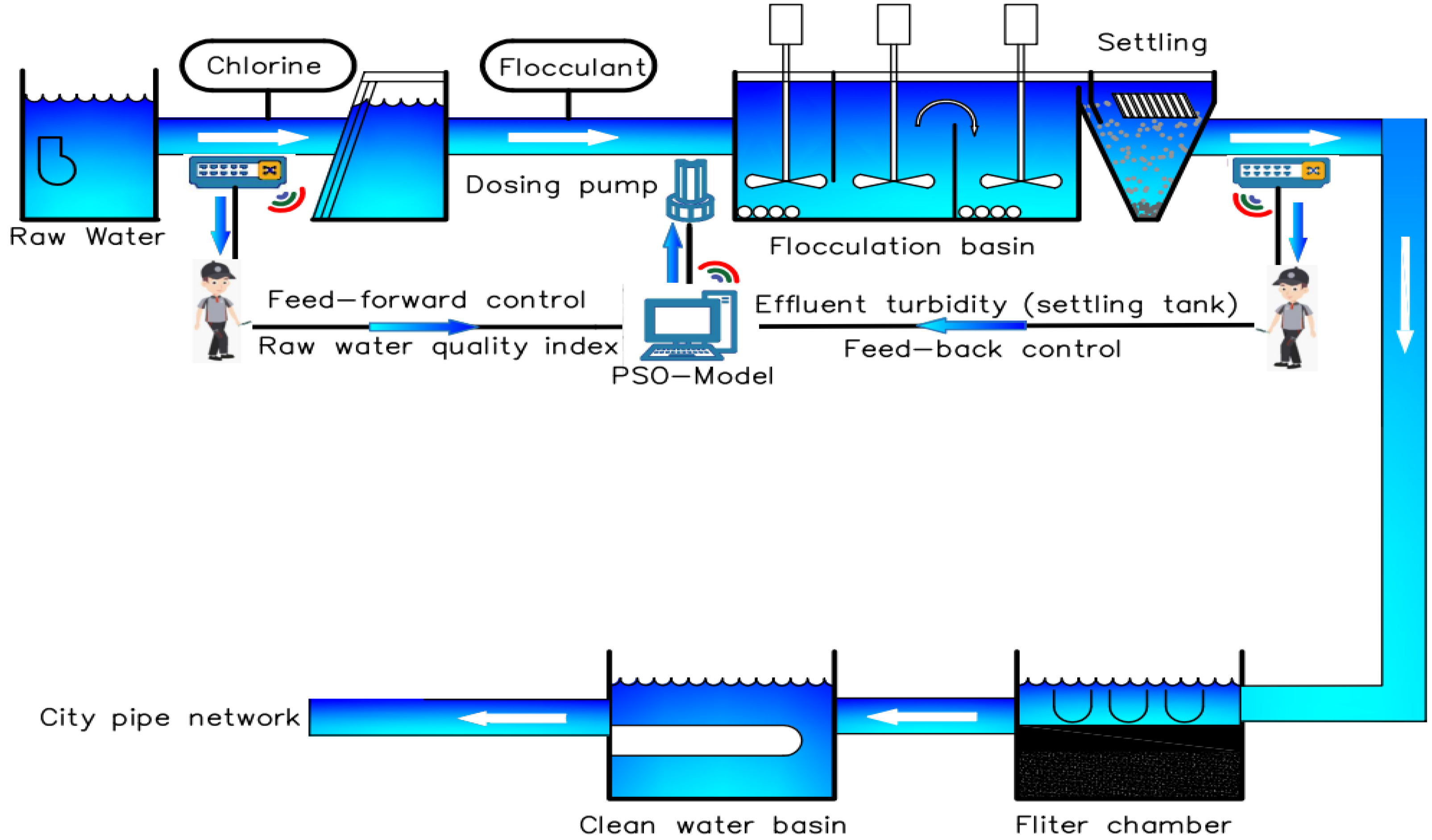
:1. Introduction
2. Materials and Methods
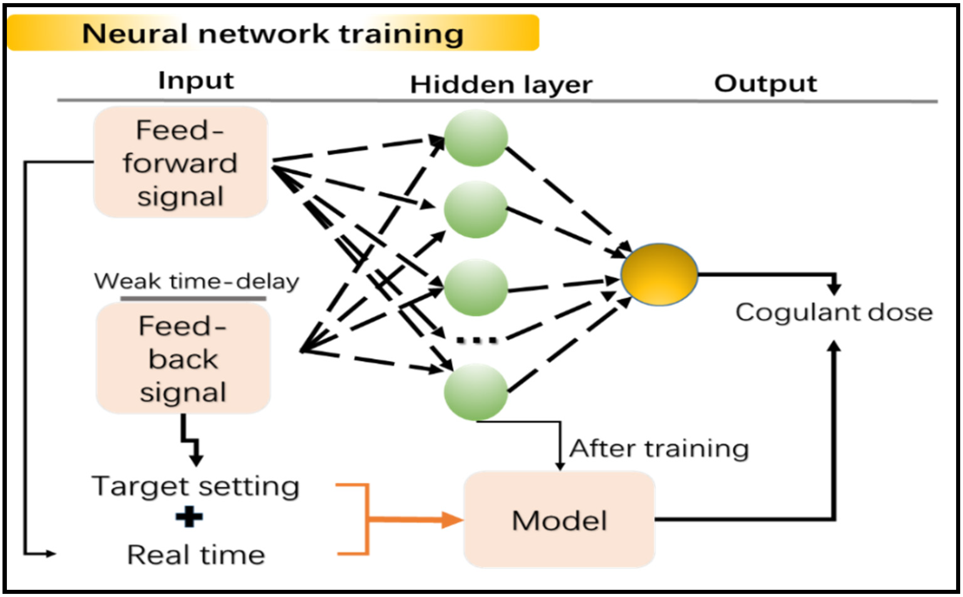
2.1. Proposed Architecture of Neural Network
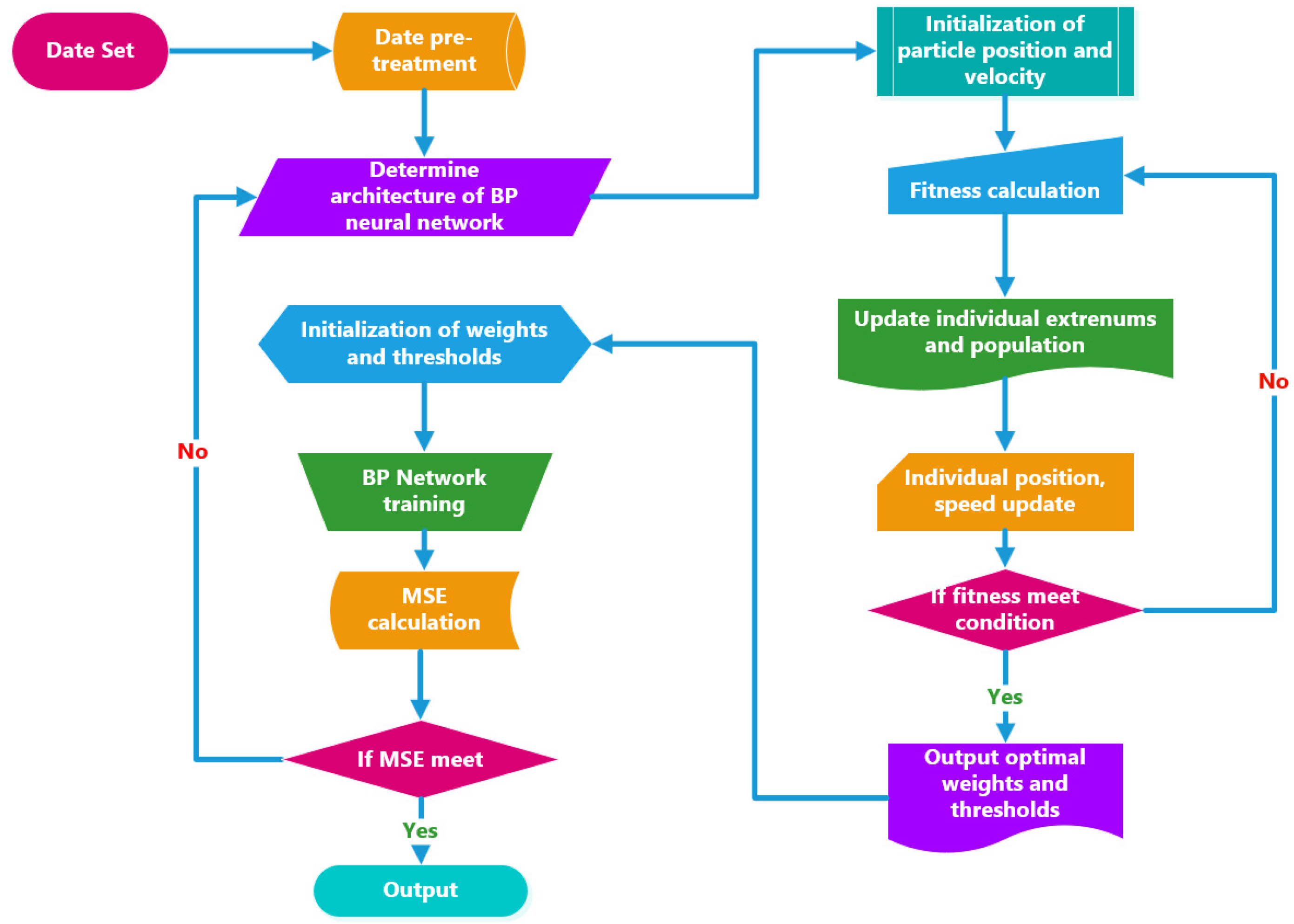
2.2. Structure Optimization
2.3. Sampling
2.4. Data Pretreatment
2.5. Accuracy
3. Results and Discussion
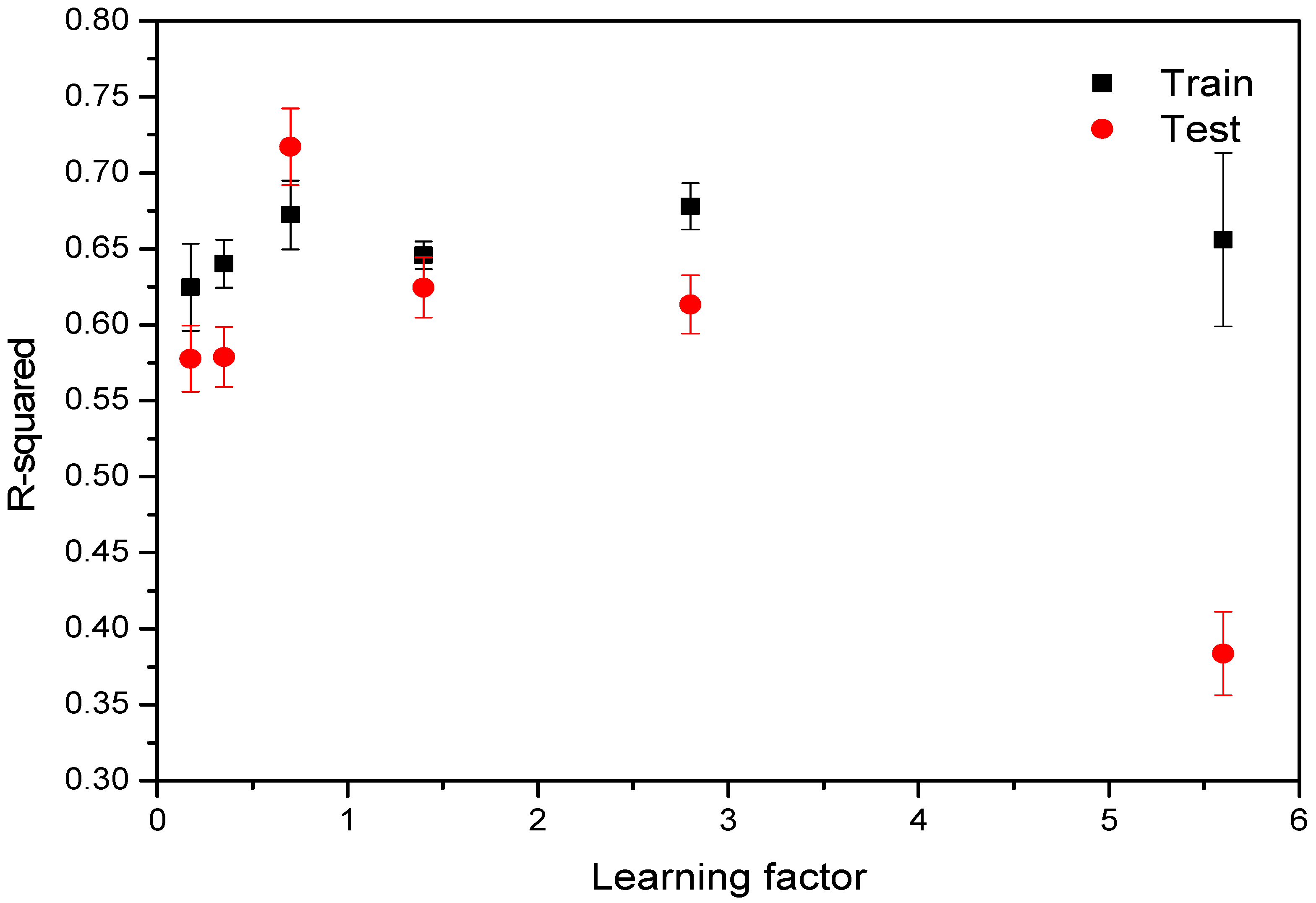
3.1. Effect of Learning Factor
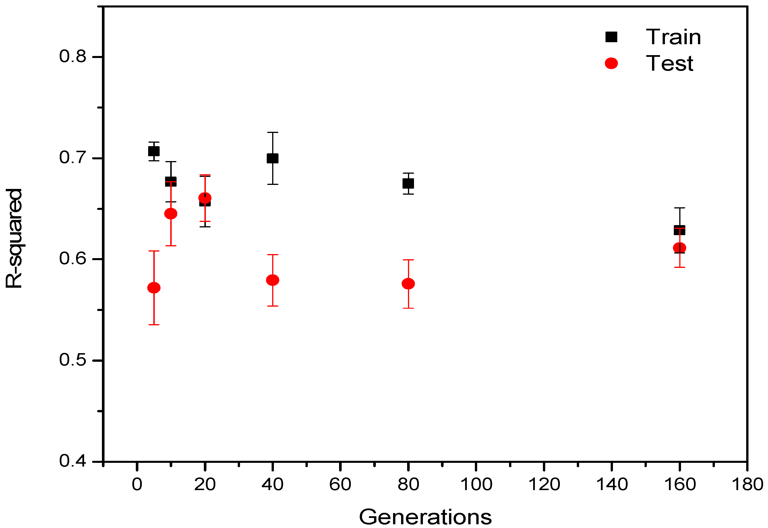
3.2. Effect of Generations
3.3. Effect of Population Size
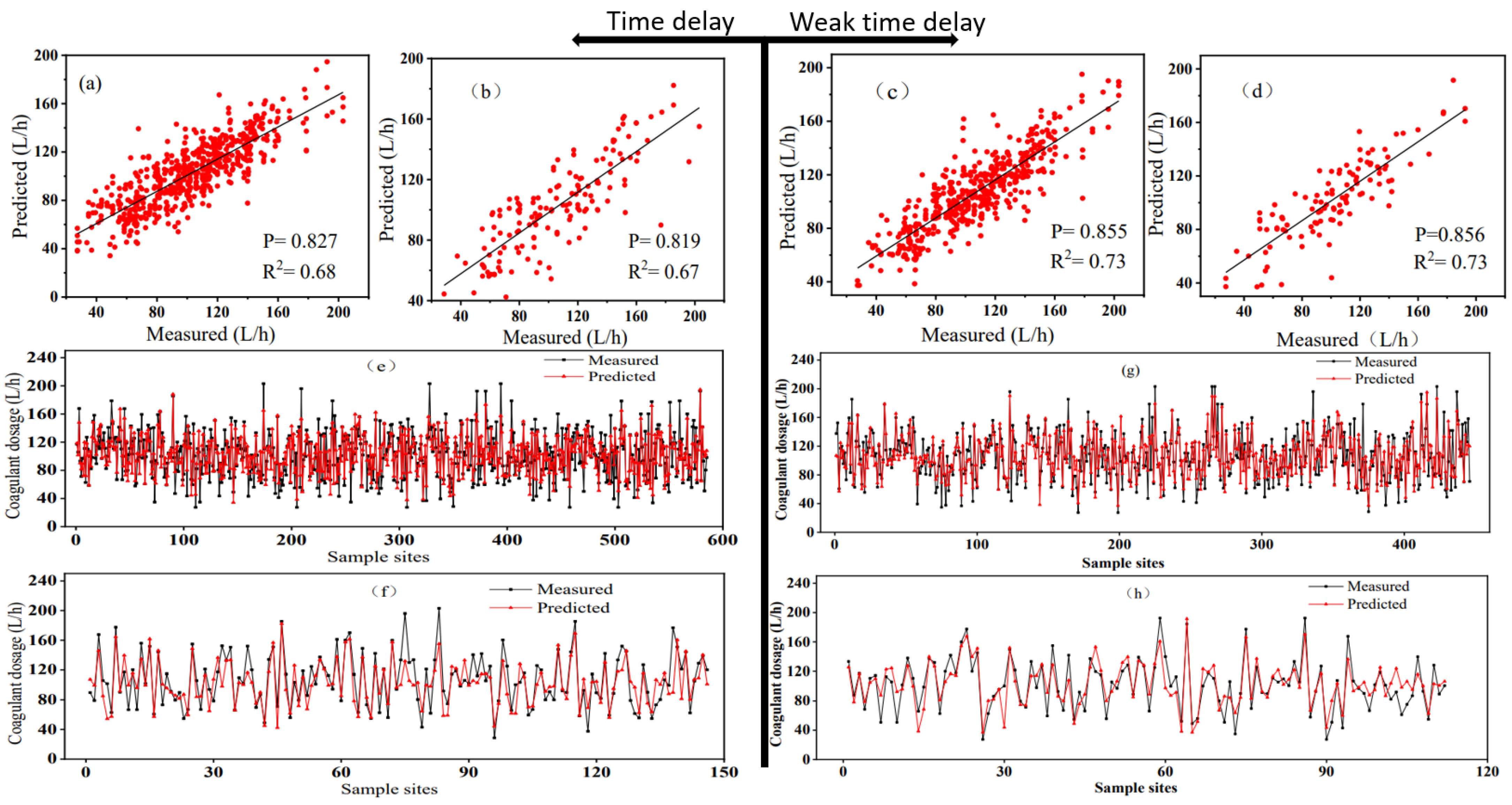
3.4. Effect of Weak Time-Delay
3.4.1. Result of Weak Time-Delay Data Training
3.4.2. Validation
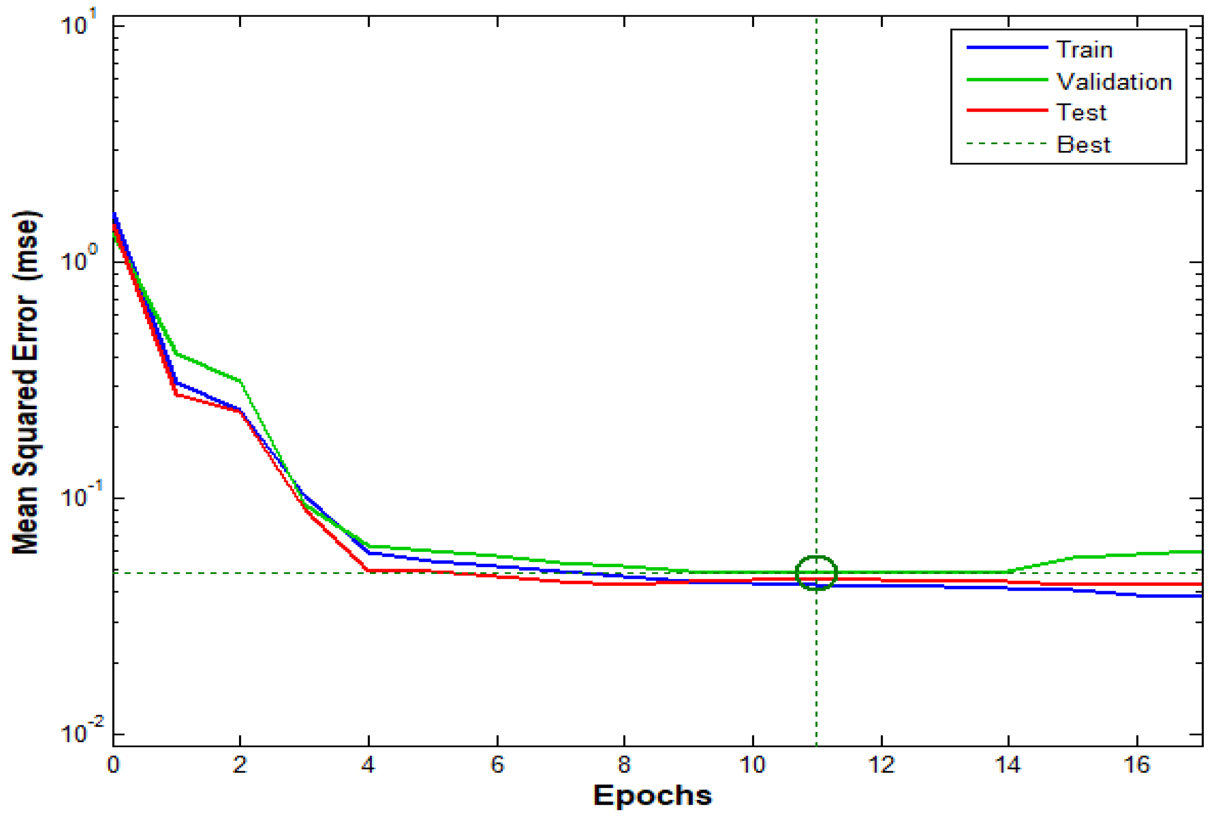
3.4.3. Variations in PSO’s Fitness and Accuracy
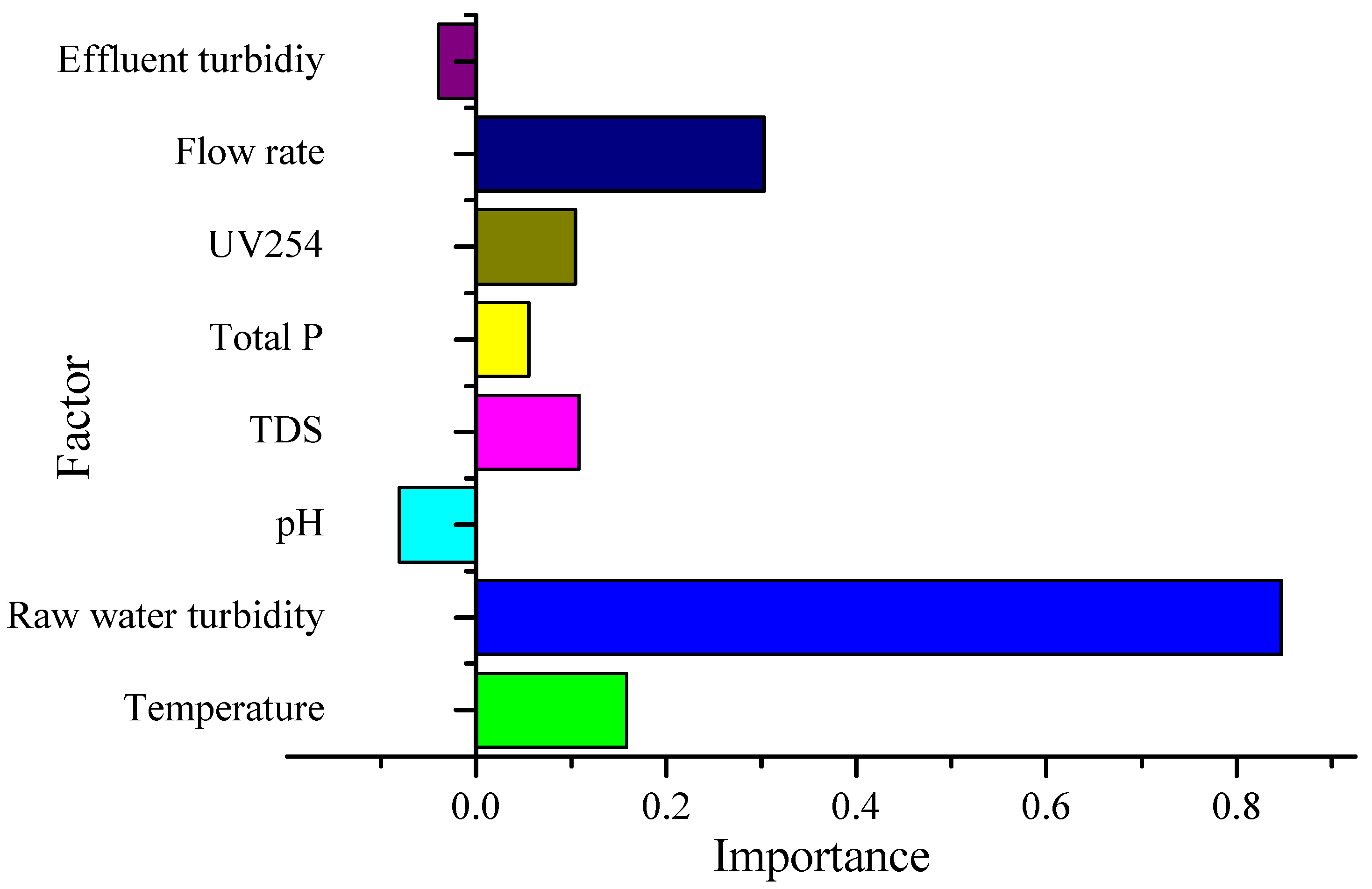
3.4.4. Sensitivity Analysis
4. Conclusions
Author Contributions
Funding
Institutional Review Board Statement
Informed Consent Statement
Data Availability Statement
Conflicts of Interest
References
- Zhang, Y.; Gao, X.; Smith, K.; Inial, G.; Liu, S.; Conil, L.B.; Pan, B.K. Integrating water quality and operation into prediction of water production in drinking water treatment plants by genetic algorithm enhanced artificial neural network. Water Res. 2019, 164, 114888. [Google Scholar] [CrossRef] [PubMed]
- Dayarathne, H.N.P.; Angove, M.J.; Aryal, R.; Abuel-Naga, H.; Mainali, B. Removal of natural organic matter from source water: Review on coagulants, dual coagulation, alternative coagulants, and mechanisms. J. Water Process Eng. 2021, 40, 101820. [Google Scholar] [CrossRef]
- Li, X.; Cheng, Z.; Yu, Q.; Bai, Y.; Li, C. Water-Quality Prediction Using Multimodal Support Vector Regression: Case Study of Jialing River, China. J. Environ. Eng. 2017, 143, 04017070. [Google Scholar] [CrossRef]
- Choo, G.; Oh, J.-E. Seasonal occurrence and removal of organophosphate esters in conventional and advanced drinking water treatment plants. Water Res. 2020, 186, 116359. [Google Scholar] [CrossRef]
- Guo, H.; Jeong, K.; Lim, J.; Jo, J.; Kim, Y.M.; Park, J.-P.; Kim, J.H.; Cho, K.H. Prediction of effluent concentration in a wastewater treatment plant using machine learning models. J. Environ. Sci. 2015, 32, 90–101. [Google Scholar] [CrossRef]
- Bai, Y.; Li, C. Daily natural gas consumption forecasting based on a structure-calibrated support vector regression approach. Energy Build. 2016, 127, 571–579. [Google Scholar] [CrossRef]
- Sezen, C.; Bezak, N.; Bai, Y.; Šraj, M. Hydrological modelling of karst catchment using lumped conceptual and data mining models. J. Hydrol. 2019, 576, 98–110. [Google Scholar] [CrossRef]
- Xiao, X.; Mo, H.; Zhang, Y.; Shan, G. Meta-ANN—A dynamic artificial neural network refined by meta-learning for Short-Term Load Forecasting. Energy 2022, 246, 123418. [Google Scholar] [CrossRef]
- Bai, Y.; Sun, Z.; Zeng, B. A multi-pattern deep fusion model for short-term bus passenger flow forecasting. Appl. Soft Comput. 2017, 58, 669–680. [Google Scholar] [CrossRef]
- Hassan, W.H.; Hussein, H.H.; Alshammari, M.H.; Jalal, H.K.; Rasheed, S.E. Evaluation of gene expression programming and artificial neural networks in PyTorch for the prediction of local scour depth around a bridge pier. Results Eng. 2022, 13, 100353. [Google Scholar] [CrossRef]
- Hassan, W.H.; Attea, Z.H.; Mohammed, S.S. Optimum layout design of sewer networks by hybrid genetic algorithm. J. Appl. Water Eng. Res. 2020, 8, 2324–9676. [Google Scholar] [CrossRef]
- Jalal, H.K.; Hassan, W.H. Effect of bridge pier shape on depth of scour[C], IOP Conference Series: Materials Science and En-gineering. IOP Publ. 2020, 671, 012001. [Google Scholar] [CrossRef]
- Odili, J.B.; Noraziah, A.; Babalola, A.E. A new fitness function for tuning parameters of Peripheral Integral Derivative Controllers. ICT Express 2021, in press. [CrossRef]
- Zhu, G.C.; Xiong, N.N.; Wang, C.; Li, Z.; Hursthouse, A.S. Application of a new HMW framework derived ANN model for optimization of aquatic dissolved organic matter removal by coagulation. Chemosphere 2021, 262, 127723. [Google Scholar] [CrossRef]
- Marzouk, M.; Elkadi, M. Estimating water treatment plants costs using factor analysis and artificial neural networks. J. Clean. Prod. 2016, 112, 4540–4549. [Google Scholar] [CrossRef]
- Li, K.; Li, L.; Qin, J.; Liu, X. A facile method to enhance UV stability of PBIA fibers with intense fluorescence emission by forming complex with hydrogen chloride on the fibers surface. Polym. Degrad. Stab. 2016, 128, 278–285. [Google Scholar] [CrossRef]
- Godo-Pla, L.; Emiliano, P.; Valero, F.; Poch, M.; Sin, G.; Monclús, H. Predicting the oxidant demand in full-scale drinking water treatment using an artificial neural network: Uncertainty and sensitivity analysis. Process Saf. Environ. Prot. 2019, 125, 317–327. [Google Scholar] [CrossRef]
- Li, L.; Rong, S.; Wang, R.; Yu, S. Recent advances in artificial intelligence and machine learning for nonlinear relationship analysis and process control in drinking water treatment: A review. Chem. Eng. J. 2021, 40, 126673. [Google Scholar] [CrossRef]
- Agudosi, E.S.; Abdullah, E.C.; Mubarak, N.M.; Khalid, M.; Pudza, M.Y.; Agudosi, N.P.; Abutu, E.D. Pilot study of in-line: Continuous flocculation water treatment plant. J. Environ. Chem. Eng. 2018, 6, 7185–7191. [Google Scholar] [CrossRef]
- Katrivesis, F.K.; Karela, A.D.; Papadakis, V.G.; Paraskeva, C.A. Revisiting of coagulation-flocculation processes in the production of potable water. J. Water Process Eng. 2019, 27, 193–204. [Google Scholar] [CrossRef]
- Alharbi, M.; Hong, P.-Y.; Laleg-Kirati, T.-M. Sliding window neural network bafsed sensing of bacteria in wastewater treatment plants. J. Process Control 2022, 110, 35–44. [Google Scholar] [CrossRef]
- Weil, M.; Mandelboim, M.; Mendelson, E.; Manor, Y.; Shulman, L.; Ram, D.; Barkai, G.; Shemer, Y.; Wolf, D.; Kraoz, Z.; et al. Human enterovirus D68 in clinical and sewage samples in Israel. J. Clin. Virol. 2017, 86, 52–55. [Google Scholar] [CrossRef] [PubMed]
- Newhart, K.B.; Holloway, R.W.; Hering, A.S.; Cath, T.Y. Data-driven performance analyses of wastewater treatment plants: A review. Water Res. 2017, 157, 498–513. [Google Scholar] [CrossRef]
- Wang, J.H.; Zhao, X.L.; Guo, Z.W.; Yan, P.; Gao, X.; Shen, Y.; Chen, Y.P. A full-view management method based on artificial neural networks for energy and material-savings in wastewater treatment plants. Environ. Res. 2022, 211, 113054. [Google Scholar] [CrossRef]
- García-Alba, J.; Bárcena, J.F.; Ugarteburu, C.; García, A. Artificial neural networks as emulators of process-based models to analyse bathing water quality in estuaries. Water Res. 2019, 150, 283–295. [Google Scholar] [CrossRef]
- Sharma, S.K.; Tiwari, K.N. Bootstrap based artificial neural network (BANN) analysis for hierarchical prediction of monthly runoff in Upper Damodar Valley Catchment. J. Hydrol. 2009, 374, 209–222. [Google Scholar] [CrossRef]
- Lin, D.; Hu, L.; Bradford, S.A.; Zhang, X.; Lo, I.M.C. Prediction of collector contact efficiency for colloid transport in porous media using Pore-Network and Neural-Network models. Sep. Purif. Technol. 2022, 290, 120846. [Google Scholar] [CrossRef]
- Onukwuli, O.D.; Nnaji, P.C.; Menkiti, M.C.; Anadebe, V.C.; Oke, E.O.; Ude, C.N.; Ude, C.J.; Okafor, N.A. Dual-purpose optimization of dye-polluted wastewater decontamination using bio-coagulants from multiple processing techniques via neural intelligence algorithm and response surface methodology. J. Taiwan Inst. Chem. Eng. 2021, 125, 372–386. [Google Scholar] [CrossRef]
- Huang, M.; Ma, Y.; Wan, J.; Wang, Y. Simulation of a paper mill wastewater treatment using a fuzzy neural network. Expert Syst. Appl. 2009, 36, 5064–5070. [Google Scholar] [CrossRef]
- Zhang, X.; He, X.; Wei, M.; Li, F.; Hou, P.; Zhang, C. Magnetic flocculation treatment of coal mine water and a comparison of water quality prediction algorithms. Mine Water Environ. 2019, 38, 391–401. [Google Scholar] [CrossRef]
- Zheng, H.; Zhu, G.; Jiang, S.; Tshukudu, T.; Xiang, X.; Zhang, P.; He, Q. Investigations of coagulation–flocculation process by performance optimization, model prediction and fractal structure of flocs. Desalination 2011, 269, 148–156. [Google Scholar] [CrossRef]
- Zangooei, H.; Asadollahfardi, G.; Delnavaz, M. Prediction of coagulation and flocculation processes using ANN models and fuzzy regression. Water Sci. Technol. 2016, 74, 1296–1311. [Google Scholar] [CrossRef] [PubMed]
- Du, J.; Shang, X.; Shi, J.; Guan, Y. Removal of chromium from industrial wastewater by magnetic flocculation treatment: Experimental studies and PSO-BP modelling. J. Water Process Eng. 2022, 47, 102822. [Google Scholar] [CrossRef]
- Baxter, C.W.; Stanley, S.J.; Zhang, Q. Development of a full-scale artificial neural network model for the removal of natural organic matter by enhanced coagulation. Aqua 1999, 48, 129–136. [Google Scholar] [CrossRef]
- Najah, A.; El-Shafie, A.; Karim, O.A.; El-Shafie Amr, H. Application of artificial neural networks for water quality prediction. Neural Comput. Appl. 2013, 22, 187–201. [Google Scholar] [CrossRef]
- Liu, H. Optimal selection of control parameters for automatic machining based on BP neural network. Energy Rep. 2022, 8, 7016–7024. [Google Scholar] [CrossRef]
- Xing, J.; Luo, K.; Pitsch, H.; Wang, H.; Bai, Y.; Zhao, C.; Fan, J. Predicting kinetic parameters for coal devolatilization by means of Artificial Neural Networks. Proc. Combust. Inst. 2019, 37, 2943–2950. [Google Scholar] [CrossRef]
- Zhou, Z.; Gong, H.; You, J.; Liu, S.; He, J. Research on compression deformation behavior of aging AA6082 aluminum alloy based on strain compensation constitutive equation and PSO-BP network model. Mater. Today Commun. 2021, 28, 102507. [Google Scholar] [CrossRef]
- Zou, X.F.; Hu, Y.J.; Long, X.B.; Huang, L.Y. Prediction and optimization of phosphorus content in electroless plating of Cr12MoV die steel based on PSO-BP model. Surf. Interfaces 2020, 18, 100443. [Google Scholar] [CrossRef]
- Li, S.; Fan, Z. Evaluation of urban green space landscape planning scheme based on PSO-BP neural network model. Alex. Eng. J. 2022, 61, 7141–7153. [Google Scholar] [CrossRef]
- Kuzenkov, O.; Kuzenkova, G. Identification of the Fitness Function using Neural Networks. Procedia Comput. Sci. 2020, 169, 692–697. [Google Scholar] [CrossRef]
- Edelmann, D.; Móri, T.F.; Székely, G.J. On relationships between the Pearson and the distance correlation coefficients. Stat. Probab. Lett. 2021, 169, 108960. [Google Scholar] [CrossRef]
- Karunasingha, D.S.K. Root mean square error or mean absolute error? Use their ratio as well. Inf. Sci. 2022, 585, 609–629. [Google Scholar] [CrossRef]
- Al-Swaidani, A.M.; Khwies, W.T.; Al-Baly, M.; Lala, T. Development of multiple linear regression, artificial neural networks and fuzzy logic models to predict the efficiency factor and durability indicator of nano natural pozzolana as cement additive. J. Build. Eng. 2022, 52, 104475. [Google Scholar] [CrossRef]
- Zhao, S.; Xu, W.; Chen, L. The modeling and products prediction for biomass oxidative pyrolysis based on PSO-ANN method: An artificial intelligence algorithm approach. Fuel 2022, 312, 122966. [Google Scholar] [CrossRef]
- Olden, J.D.; Joy, M.K.; Death, R.G. An accurate comparison of methods for quantifying variable importance in artificial neural networks using simulated data. Ecol. Model. 2004, 178, 389–397. [Google Scholar] [CrossRef]


| Type | R2 | RMSE | RMSE% | PBIAS | EF | d |
|---|---|---|---|---|---|---|
| Weak time-delay train | 0.73 | 17.97 | 16.90 | 0.00 | 0.73 | 0.91 |
| Weak time-delay test | 0.73 | 18.15 | 17.76 | 0.00 | 0.73 | 0.91 |
| Time-delay train | 0.68 | 19.08 | 18.58 | 0.00 | 0.68 | 0.89 |
| Time-delay test | 0.67 | 21.10 | 19.73 | 0.00 | 0.65 | 0.89 |
Publisher’s Note: MDPI stays neutral with regard to jurisdictional claims in published maps and institutional affiliations. |
© 2022 by the authors. Licensee MDPI, Basel, Switzerland. This article is an open access article distributed under the terms and conditions of the Creative Commons Attribution (CC BY) license (https://creativecommons.org/licenses/by/4.0/).
Share and Cite
Luo, H.; Li, X.; Yuan, F.; Yuan, C.; Huang, W.; Ji, Q.; Wang, X.; Liu, B.; Zhu, G. Application of a New Architecture Neural Network in Determination of Flocculant Dosing for Better Controlling Drinking Water Quality. Water 2022, 14, 2727. https://doi.org/10.3390/w14172727
Luo H, Li X, Yuan F, Yuan C, Huang W, Ji Q, Wang X, Liu B, Zhu G. Application of a New Architecture Neural Network in Determination of Flocculant Dosing for Better Controlling Drinking Water Quality. Water. 2022; 14(17):2727. https://doi.org/10.3390/w14172727
Chicago/Turabian StyleLuo, Huihao, Xiaoshang Li, Fang Yuan, Cheng Yuan, Wei Huang, Qiannan Ji, Xifeng Wang, Binzhi Liu, and Guocheng Zhu. 2022. "Application of a New Architecture Neural Network in Determination of Flocculant Dosing for Better Controlling Drinking Water Quality" Water 14, no. 17: 2727. https://doi.org/10.3390/w14172727