
Evaluation of Hydrological Rainfall Loss Methods Using Small-Scale Physical Landslide Model


1
Faculty of Civil and Geodetic Engineering, University of Ljubljana, 1000 Ljubljana, Slovenia
2
Faculty of Civil Engineering, University of Rijeka, 51000 Rijeka, Croatia
*
Author to whom correspondence should be addressed.
Water 2022, 14(17), 2726; https://doi.org/10.3390/w14172726
Submission received: 28 July 2022
/
Revised: 24 August 2022
/
Accepted: 30 August 2022
/
Published: 1 September 2022
(This article belongs to the Special Issue Hydrological Modeling of Landslides and Debris Flows)
Abstract
:An adequate representation of the relationship between effective rainfall and rainfall losses is required in hydrological rainfall–runoff models to reduce the uncertainty of the modelling results. This study evaluates the performance of several hydrological rainfall loss methods using the experimental data obtained from a laboratory small-scale physical landslide model with variable slope inclination, homogenous material and no vegetation effects. Three different experiments were selected and five rainfall loss methods were tested to evaluate their performance in reproducing the experimental results from the perspective of the surface runoff formation on the experimental slope. Initial and calibrated parameters were used to test the performance of these hydrological rainfall loss methods. The results indicate that the initial parameters of the rainfall loss model can satisfactorily reproduce the experimental results in some cases. Despite the fact that the slope material characteristics used in the laboratory experiments were relatively homogenous, some well-known methods yielded inaccurate results. Hence, calibration of the rainfall loss model proved to be essential. It should also be noted that, in some cases, the calibrated model parameters were relatively different from the initial model parameters estimated from the literature. None of the tested hydrological rainfall loss methods proved to be superior to the others. Therefore, in the case of natural environments with heterogeneous soil characteristics, multiple rainfall loss methods should be tested and the most suitable method should be selected only after cross-validation or a similar evaluation of the tested methods.
1. Introduction
Extreme rainfall is one of the main drivers of water-related disasters such as floods, flash floods, extreme soil erosion and landslides [1,2,3,4,5,6,7]. In terms of analyzing flood generation mechanisms, rainfall is often separated into effective rainfall, which contributes to the increasing part of the hydrograph during and soon after a rainfall event, and rainfall losses [8]. The rainfall losses can be regarded as a part of precipitation that does not directly contribute to the surface or sub-surface runoff or that does not increase the hydrograph during or immediately after the precipitation event [8,9,10]. Hence, rainfall losses are part of the precipitation that is either intercepted by vegetation or infiltrated into soil. The separation of the total rainfall into effective rainfall and rainfall losses needs to be correctly represented within the hydrological rainfall–runoff models.
Rainfall–runoff modelling is widely used in hydrology and related disciplines for various purposes, such as flood prediction, the design of flood protection measures or climate change investigations [11,12,13,14,15]. In addition, there are various rainfall–runoff models available, including physically based, conceptual, empirical and data-driven models [16,17,18]. Hence, each of these models has its own characteristics, including data requirements, model structure, complexity and a representation of the effective rainfall–rainfall loss relationship [17]. One of the most frequently applied models in engineering hydrology is the Hydrological Engineering Center (HEC) Hydrologic Modeling System (HMS), or, in short, HEC-HMS software [9]. This software includes a variety of methods that can be used for relatively simple event-based rainfall–runoff calculations using the unit hydrograph (UH) theory, or to conduct more complex continuous or even grid-based modelling of various rainfall–runoff processes [9]. In the scope of engineering applications related to design discharge and hydrograph estimation, which are often carried out with the HEC-HMS software [14,19,20], a suitable method for the calculation of rainfall losses must also be chosen.
Within the HEC-HMS model, there are several methods available, such as Green and Ampt’s model or the initial and constant method, which can be used to estimate rainfall losses [8,9]. Some of them are suitable for event-based simulations and others for continuous rainfall–runoff modelling [9]. Additionally, these methods mostly use different infiltration process theories, which can be found in the literature [21]. These models describing infiltration are either empirical (e.g., Horton infiltration model) or physically based (e.g., Green and Ampt model) [21]. Previous studies have shown that different methods that are incorporated into the HEC-HMS can yield very diverse results in terms of estimating the effective rainfall (the part of the rainfall that contributes to runoff) [8,22,23]. Therefore, additional investigations are needed to evaluate the performance of specific methods. Such evaluations can be undertaken based on large datasets including rainfall and discharge data for various catchments (e.g., as part of national hydro-meteorological monitoring systems [13,24]), using detailed measurements from experimental catchments [25,26,27], considering data obtained from laboratory experiments [28,29] or a combination of data from laboratory experiments and experimental catchments [30].
Laboratory experiments are also frequently used in the context of studying the dynamics of landslides and the effects of landslide remediation measures [31,32,33,34,35,36,37,38]. Hence, the focus of this type of experiment is usually not only on the relationship between rainfall, soil moisture, infiltration and runoff, despite their relative importance for the initiation of rainfall-induced landslides [39,40]. The focus is often on the investigation of landslide dynamics and on understanding landslides’ initiation mechanisms [31,32]. These issues are important for the communities affected by landslides, since landslides are one of the natural hazards that can occur almost anywhere around the globe [41], in various types and magnitudes [42]. Additionally, landslides can cause significant economic damage and endanger human lives [43,44]. Moreover, understanding landslide behavior, modelling, mitigation and prediction are becoming more and more important in order to increase social resilience, and also due to the climate change impact, which is expected to affect landslide frequency and dynamics [45,46,47,48]. Interdisciplinary research, such as combining hydrological aspects with experimental data from laboratory landslide tests, can therefore provide new insights from which multiple scientific disciplines can benefit.
Therefore, the main aim of this study is to evaluate the performance of different methods that can be used to estimate rainfall losses based on measurements taken within small-scale landslide laboratory experiments. More specifically, we tested the hypothesis that estimating rainfall loss parameters based on the literature can provide a valuable representation of conditions during laboratory experiments. We also investigated whether the calibrated rainfall loss parameters can reproduce the observed experimental results. The secondary objective of the study was to analyze how soil moisture changed during the laboratory experiments with respect to slope geometry and soil material characteristics.
2. Methods
2.1. Laboratory Landslide Experiments
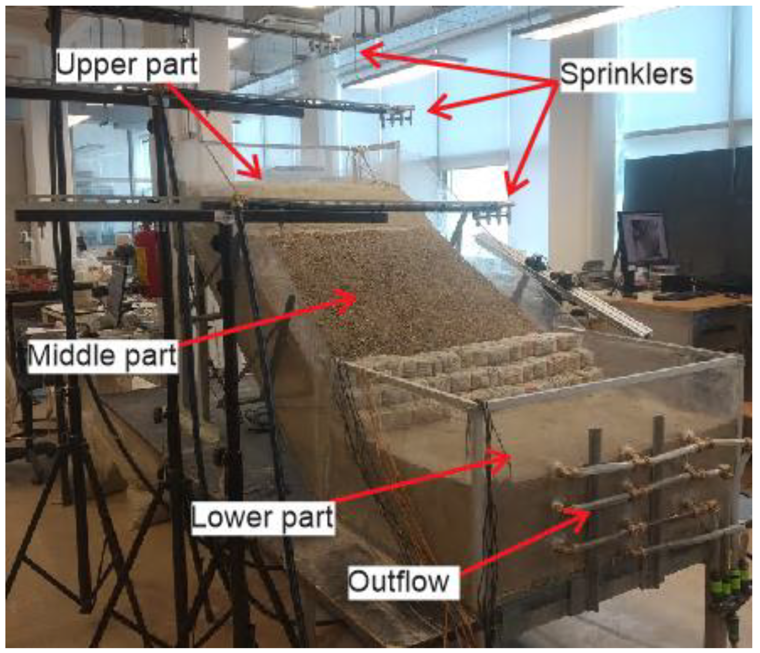
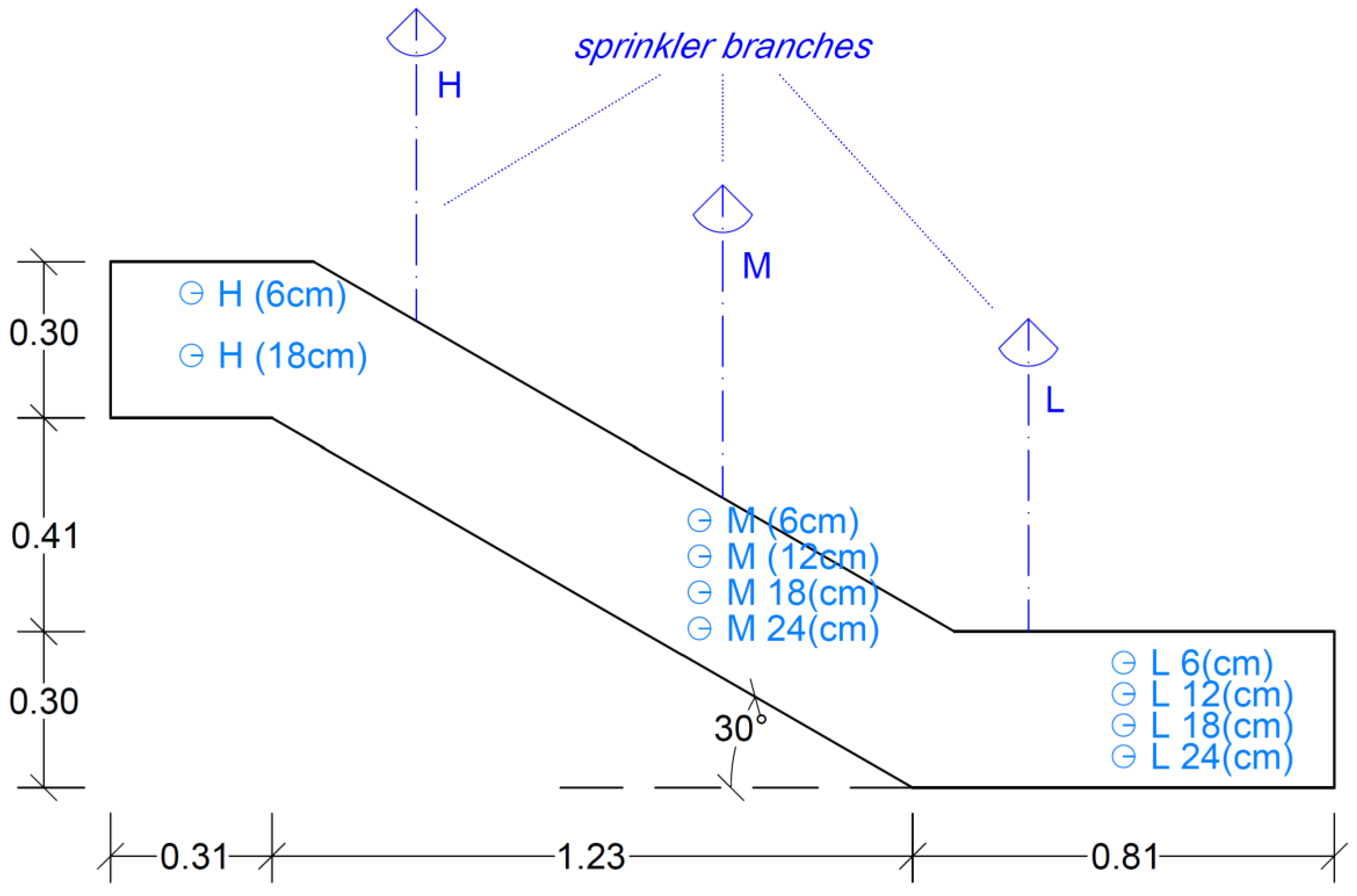
In the scope of this study, we used the results of the physical landslide model experiments described in detail in previous studies [31,32,49]. A platform for testing small-scale physical landslide models was developed within a four-year research project entitled “Physical modeling of landslide remediation constructions’ behavior under static and seismic actions (ModLandRemSS)”. This platform was designed to investigate the landslide triggering mechanisms and the effects of landslide remediation measures on the stability of slopes. The experimental setup is equipped with extensive geotechnical and geodetic monitoring systems that are able to measure multiple variables, such as soil moisture, suction, pore pressures and displacements [31]. Hence, numerous accelerometers, strain gauges, pore pressure transducers and soil moisture probes are used to measure these variables [31]. In addition, infrared cameras, high-speed cameras, terrestrial laser scanners and Structure-from-Motion (SfM) photogrammetry were used to detect displacements, landslide failure mechanisms and patterns during the experiment [31]. A detailed description of the geodetic and geotechnical monitoring systems and the sensors used is provided by Pajalić et al. [31] and Peranić et al. [50]. It should be noted that all water-related sensors were produced by the METER Group company, and TEROS 10 and TEROS 12 sensors were employed for soil moisture measurements [31]. These sensors were also used in the scope of this study. Figure 1 shows the main elements of the small-scale physical model. The model consists of a steel base plate with side elements made of transparent plexiglass [31]. The dimensions of the slope are 1 m (width), 2.3 m (length) and 0.5 m (height) [31]. A schematic representation of the physical model’s cross-section with the position of the soil moisture sensors is presented in Figure 2. The model slope can be modified and a series of tests were performed using inclinations of 30°, 35° and 40°. A detailed description of the preparation of the model experiment and material (e.g., achieving the targeted compaction and moisture conditions) is available in previous publications [31,32,49].
The rainfall simulator used in the setup shown in Figure 2 is one of the main elements that was constructed specifically to provide variable water pressure and hence variable rainfall intensities during the experiments [31]. As can be seen in Figure 1, three sprinkler branches, each equipped with four different axial-flow nozzles with spray angles of 60° and 90°, were used to produce controlled artificial rainfall events. The height of the sprinklers above the model was determined by considering rainfall spread in such a way that water reached the edges of the model during the experiments. The rainfall intensities can vary from 30 to 140 mm/h [31]. Starting rainfall intensities used during the experiments were determined based on the infiltration capacity of different slope materials. The maximum values of rainfall intensity that can infiltrate into the soil without the appearance of surface runoff were selected for each specific experiment, as described in the following sections.
Multiple experiments have been conducted using three different slope materials, where their properties are shown in Table 1. Besides clean uniform sand, two sand–kaolin mixtures, one with 10% and one with 15% of kaolin particles, were used to build scaled slope models (Table 1). The kaolin mixtures were determined based on weight (mass) proportions of sand and kaolin. The grain size distribution curve included the distribution of soil particles of different sizes in the soil mass. Grain size distribution curves and other material properties are presented in Vivoda Prodan et al. [49]. Dynamic responses of models built of different soil types and with different inclinations (30°, 35° and 40°) were observed and measurements were taken during the experiments. Moreover, to observe differences in the dynamic responses of scaled slope models with and without different remediation measures, the tests were also repeated with specific landslide remediation measures applied, such as gabion and gravity retaining walls, piles, etc. [51].
2.1.1. Data Used for Rainfall Loss Simulations
Three experiments were selected for the assessment of the applicability of selected rainfall loss methods (Section 2.2):
- Experiment with sandy material with 35° inclination, where surface runoff was observed during the experiment after increasing the rainfall intensity during the second part of the experiment (Sand).
- Experiment with a mixture of sand and 10% kaolin with a 40° inclination, where the initial moisture of the material was relatively high (volumetric water content of approximately 0.2 m3/m3) and surface runoff (and erosion) was observed shortly after the start of the experiment (SK10er).
- Experiment with a mixture of sand and 10% kaolin with a 40° inclination, where the initial moisture content of the material was lower (approximately 0.06 m3/m3) than in the previously selected experiment and where no surface runoff was observed during the experiment (SK10).
The above considered combinations represent various conditions (e.g., higher initial moisture, increase in the rainfall intensity during the event). It should be noted that the rainfall intensity for the experiment Sand was slightly higher (around 3 L/min) than for the experiments SK10er and SK10 (around 0.8 L/min), as shown in Section 3. As indicated, initial rainfall intensities used during specific experiments were determined based on the infiltration capacity of different slope materials. During the experiments, rainfall intensity was reduced when the ground water level reached the ground surface in the lowest part (foot) of the model and the foot of the slope was submerged. In the last part of the experiment Sand, when most of the expected slope movements were reached, the rainfall intensity was increased above the soil infiltration capacity in order to observe the joint impact of infiltration and surface runoff on the slope behavior.
2.1.2. Data Used for Investigation of Soil Moisture Changes
Additionally, we also investigated soil moisture dynamics at various depths (Figure 2) with respect to the inclination of the model and the material characteristics. Appropriate combinations were selected considering two conditions: (i) the rainfall intensity was the same during different experiments and (ii) the initial soil moisture was similar between different experiments. The following combinations were compared:
- Sandy material for 35° and 40° inclinations with an initial approx. rainfall intensity of 3 L/min;
- Sandy material with 10% kaolin for 35° and 40° inclinations with an initial rainfall intensity of approx. 0.8 L/min.
2.2. Methods for the Evaluation of the Rainfall Losses
HEC-HMS software [9] was used for the estimation of rainfall losses for the selected methods, with the exception of the Horton infiltration method, which is not incorporated into the HEC-HMS (Section 2.2.5). Four methods that can be used for event-based simulations were selected [9]: Green and Ampt, Smith Parlange, initial and constant and Soil Conservation Service (SCS) methods. Descriptions of these methods, including the Horton infiltration model, are provided in the following sub-sections.
2.2.1. Green and Ampt
The Green and Ampt method can be regarded as a physically based model and is, in general, a simplification of a more complex equation for unsteady water flow in soils proposed by Richards [9,21,52,53,54]. Within the HEC-HMS software, the Green and Ampt method uses the so-called piston-type displacement for the movement of the infiltrated water by the approximation of the wetting front [9]. Initially, the soil is assumed to be uniformly saturated in the case of this method. In the case of conducted experiments, there were smaller variations in the initial soil moisture because of the water movement and evaporation during the experiment preparation (see Section 3 for further details). The soil is also assumed to be infinitely deep (only the Green and Ampt equation can be used for defining the saturation point); the Green and Ampt model also takes into consideration ponding at the soil–air interface [9]. The rainfall losses for specific time intervals are calculated within the HEC-HMS model using the following expression [9]:
where K is the saturated hydraulic conductivity, is the rainfall loss during the time step t, is the volume moisture deficit, is the cumulative loss at time t and is the wetting front suction. Parameters required by the HEC-HMS software are [9]:
- Initial content (m3/m3);
- Saturated content (m3/m3);
- Suction (mm);
- Conductivity (mm/h).
In our case, the initial moisture content was defined based on the soil moisture measurements (METER group sensors) before the start of an experiment (Section 2.1). The saturated content defines the maximum water holding capacity from the perspective of the volume ratio and can be estimated based on the total porosity [9]. Furthermore, the suction parameter is related to the wetting front suction head and represents the attraction of water within the material void spaces [9]. Hence, this parameter can be estimated either based on the soil texture information or the soil water retention curve (wetting phase). Moreover, the conductivity parameter is the saturated hydraulic conductivity that represents the rate at which water from the surface enters soil when completely saturated [9]. Table 2 shows the estimated Green and Ampt parameters that were determined based on the material characteristics and literature information.
2.2.2. Smith Parlange Method
The second method that was selected for the calculation of the rainfall losses is the Smith Parlange model, which is also suitable for event-based simulations [9]. This method is a simplification of the Richards equation, with the assumption that the wetting front can be represented by the exponential scaling of saturated conductivity [9]. The potential infiltration rate at specific time steps within the HEC-HMS model can be calculated using the following expression [8]:
where KS is the effective saturated hydraulic conductivity within a time step, B is the saturation deficit parameter and fcum is the cumulative infiltration since the start of the event [8]. Parameters required within the HEC-HMS software in relation to the Smith Parlange method are [9]:
- Initial content (m3/m3);
- Residual content (m3/m3);
- Saturated content (m3/m3);
- Bubbling pressure (mm);
- Pore distribution;
- Conductivity (mm/h).
The initial and saturated content are similar to the Green and Ampt method (Section 2.2.1), while the residual water content is determined by the amount of water remaining in the soil after drainage [9]. Moreover, the bubbling pressure represents the wetting from suction. Additionally, the pore size distribution can be related to the soil texture [55] and defines the distribution of total pore spaces in different size classes [9]. For the conductivity parameter, typically, the effective saturated conductivity is used [9]. The HEC-HMS software also includes an option to adjust the water density, viscosity and matric potential based on the provided temperature data, which was not used within the simulations performed within the scope of this study. Table 3 shows the estimated Smith Parlange parameters that were estimated based on the material characteristics and literature information.
2.2.3. Initial and Constant Method
The third method that was used for the comparison was the initial and constant loss method, which can be regarded as a simpler empirical method compared to the Green and Ampt and the Smith Parlange methods. The method is more suitable for cases with limited soil information [9]. The method uses a single soil layer and the initial loss can be specified in order to represent the amount of water that is expected to be lost before the onset of runoff infiltration [9]. In other words, until the accumulated precipitation is equal to the initial loss value, no runoff will be simulated. After this period, the runoff will be simulated when the precipitation rate is higher than maximum potential rate of rainfall loss. Two parameters need to be defined in relation to this method within the HEC-HMS software [9]:
- Initial loss (mm);
- Constant rate (mm/h).
The initial loss parameter represents the amount of precipitation that is expected to be infiltrated before the start of the runoff and can be estimated as the product of the active layer depth (in our case, 30 cm of the material) and soil moisture state at the start of the simulation. This parameter can also be estimated based on the land use by using some pre-defined values [9]. In our case, the initial loss parameter was calculated as the ratio between the active layer depth and the difference between the saturated and initial content (Table 2). Additionally, the constant rate is usually assumed to be equal to the saturated hydraulic conductivity [9]. Table 4 shows the estimated initial and constant method parameters that were estimated based on the material characteristics and literature information.
2.2.4. Soil Conservation Service (SCS) Method
The fourth method that was selected was the SCS model, which is derived based on the water balance equation. The method was derived to calculate the total infiltration during a storm and uses only one parameter: the curve number (CN) [9,21]. It is one of the most frequently used in engineering hydrology since the CN parameter can be estimated based on the land use and soil characteristics [8]. The CN concept has also been used for several other purposes [56,57]. The calculated cumulative rainfall excess Pe can be calculated using:
where P is the accumulated rainfall at time step t; the S and Ia coefficients represent the maximum retention and initial abstraction, respectively. Both parameters can be calculated based on the CN parameter [8,9]. The HEC-HMS user’s manual provides a table with pre-defined CN parameters for various land cover types and for four different soil classes that can be related to the soil texture (A, B, C and D) [8,9]. Additionally, a specific initial abstraction Ia can be provided; otherwise, this parameter is calculated based on the provided CN value. In our study, the initial CN parameters were determined as representing areas without vegetation. For the experiment with sand, soil type A was assumed (CN = 77), and for the experiment on sand with 10% kaolin, soil type B was assumed (CN = 86).
2.2.5. Horton Infiltration Method
The last method that was used was the Horton infiltration method, which can be regarded as empirically based [21]. It is one of the most frequently used methods and assumes that infiltration is decreasing exponentially from the initial capacity to the final one. The method and the work conducted by Horton have been widely studied [58,59]. The infiltration rate f at time t can be calculated as [8]:
where f0 is the initial infiltration, fc is the final infiltration and k is a constant that represents the decrease in infiltration capacity. Table 5 shows the estimated Horton model parameters that were estimated based on the material characteristics and literature information [60].
2.3. Evaluation of Five Selected Rainfall Loss Methods Based on the Laboratory Experiments
For the evaluation of the applicability of the five rainfall loss methods (Section 2.2) for the selected experiments (Section 2.1.1), we have used the following steps:
- The initial rainfall loss methods’ parameters were estimated based on model material characteristics, initial measurements before the start of the experiment and literature information.
- The rainfall losses were estimated using the initial model parameters (previous step) and comparison with the experimental results was made with respect to the timing and occurrence of surface runoff.
- The rainfall loss parameters were calibrated in such a way that the experimental results could be reproduced with respect to the timing of the occurrence or non-occurrence of surface runoff. Evaluation of the calibrated parameters was conducted to see if the calibrated parameters were within a plausible range of the parameters according to the material characteristics. In other words, we were interested in whether the calibrated parameters for sandy material were within a range of parameters for this type of material or whether they correspond to completely different soil types (e.g., clay).
It should be noted that, in almost all cases, the HEC-HMS software user’s manual indicates that rainfall loss parameters for all the selected methods should be calibrated before conducting simulations.
Evaluation was performed using a ranking system ranging from 0 to 3, where the following system was used:
- 0 was used if simulated runoff was completely different from the experimental results (e.g., no runoff was simulated while runoff appeared during the experiment).
- 1 was used if simulations correctly predicted runoff occurrence for one part of the experiment (e.g., HEC-HMS simulations predicted runoff but missed the correct timing in comparison to the actual experimental results).
- 2 was used if simulations correctly predicted runoff (occurrence) and the timing of runoff for one part of the experiment but did not correctly predict runoff for another part of the experiment.
- 3 was used if simulations were completely in accordance with the experimental results.
2.4. Interpretation of Soil Moisture Changes during the Experiments
In relation to the second aim of the study, we also investigated changes in soil moisture at various locations and depths within the model for the selected combinations of model slope and material characteristics (Section 2.1.2). Hence, visualization was performed using scatter plots and relatively simple descriptive statistics were calculated to compare different experiments.
3. Results and Discussion
3.1. Evaluation of the Rainfall Loss Methods
3.1.1. Initial Model Parameters
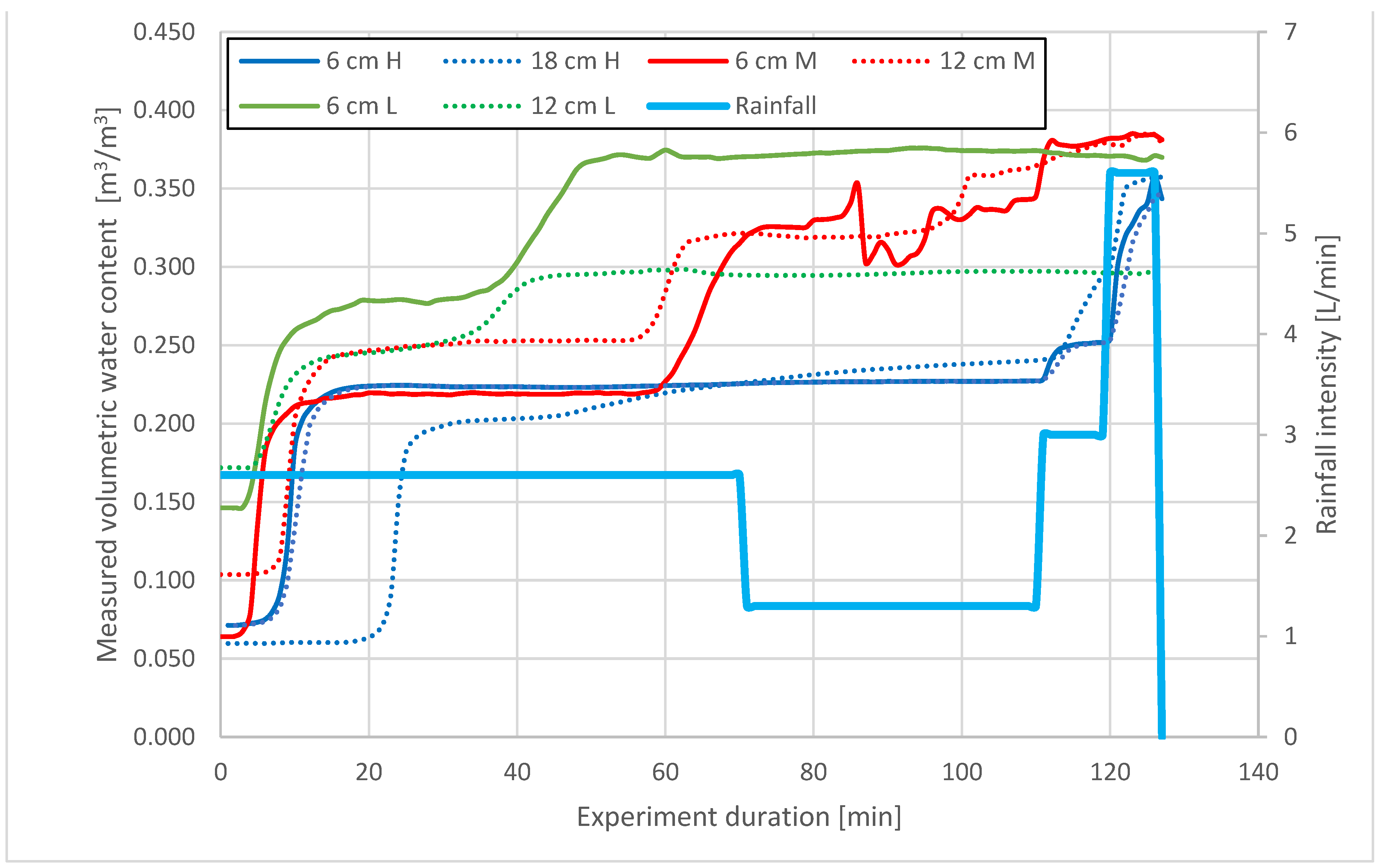
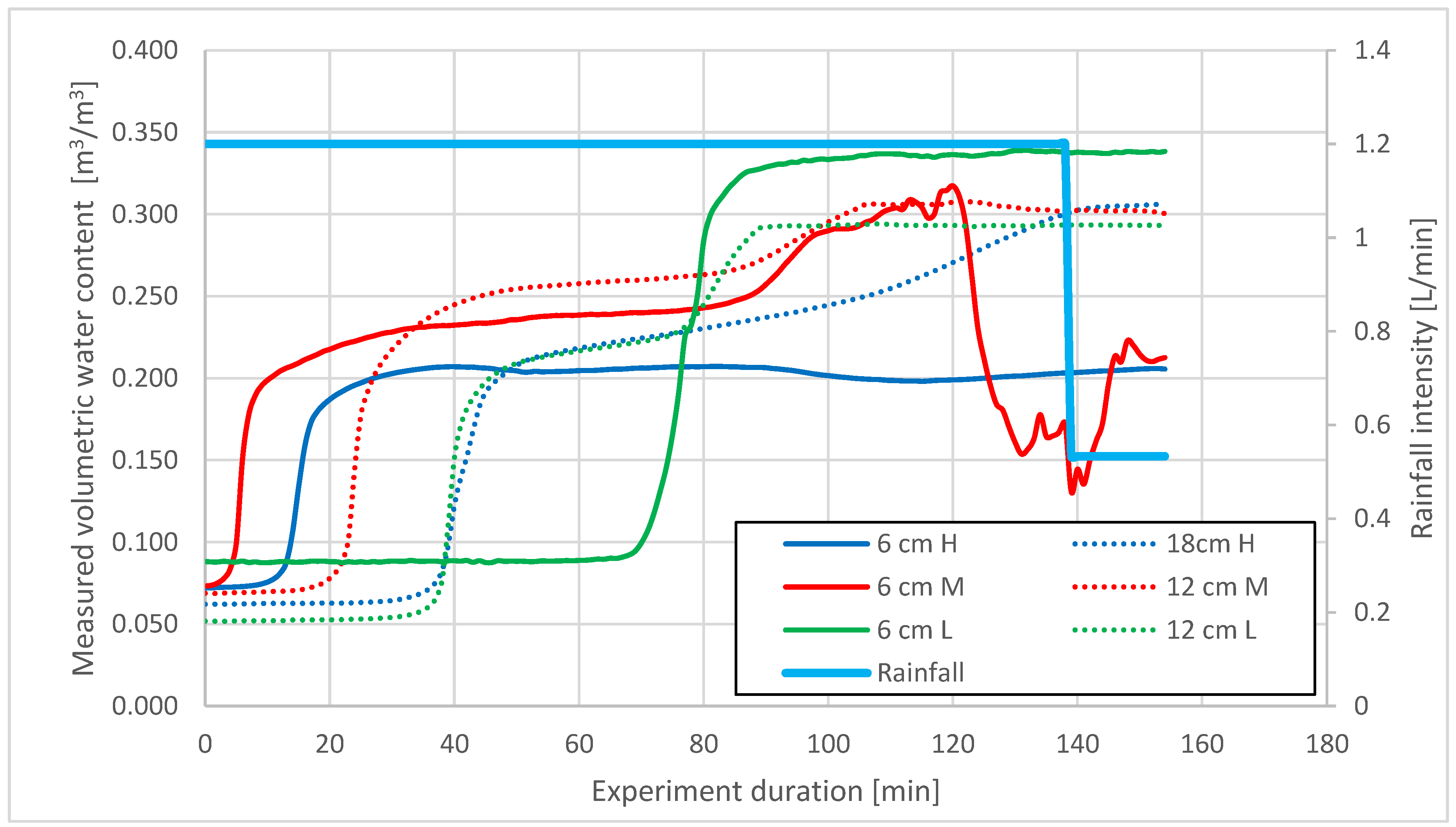
Firstly, we evaluated the performance of the selected rainfall loss methods using the initial parameters (Table 6). In the case of the experiment where sand (Sand) was used, all the methods yielded relatively similar performance according to the selected rank-based evaluation (Table 6). Hence, in this experiment, the surface runoff (in the upper part of the model: H section) started after an increase in the rainfall intensity during the last part of the experiment (Figure 3 and Figure 4). Hence, the surface runoff occurred at the point where the volumetric water content exceeded 0.25 m3/m3 and 0.35 m3/m3 in the upper part (H section) and middle part (M section) of the model, respectively. Meanwhile, the value of 0.35 m3/m3 was exceeded after around 50 min of the experiment in the lower part of the model as a result of water ponding in this part of the small-scale model. All the selected rainfall loss methods, with the exception of the initial and constant method, predicted the start of the surface runoff at around 15–20 min, where the volumetric water content quickly increased during the experiment (Figure 3). The first cracks during the experiment occurred around 30 min after the start of rainfall. Moreover, all the methods correctly predicted the increase in the surface runoff in the last part of the experiment, when the rainfall intensity was increased (Figure 3). The Green and Ampt method was the only method that predicted the end of the surface runoff at the middle part of the experiment (after around 1 h and before the increase in the rainfall intensity), while, in the case of the Smith Parlange, SCS curve number and Horton infiltration methods, the surface runoff did not stop until the end of the experiment. The initial and constant method was the only one that did predict the start of the runoff in the last part of the experiment (Figure 3 and Figure 4). Hence, in the case of this experiment, the results using the initial parameters for this method seem to slightly better reproduce the experimental results compared to some more complex methods that were tested (Table 6).
In the case of the second experiment that was taken into consideration (SK10), where no surface runoff could be observed during the experiment, the Green and Ampt, Smith Parlange and initial and constant methods yielded similar results and did not predict any surface runoff. On the other hand, the SCS curve number predicted the start of the surface runoff at around 20 min after the start of the rainfall, which corresponds relatively well to an increase in the volumetric water content at the upper and middle parts of the model (Figure 5). In this case, the volumetric water content increased by over 0.2 m3/m3. Moreover, the Horton infiltration method predicted the start of the runoff from the beginning of the rainfall, which is not in accordance with the experimental results. It should be noted that the second increase in the volumetric water content in the period from 40 to 80 min from the start of the experiment can be associated with the appearance of the first cracks in the model. None of the selected rainfall loss methods, except the SCS CN method, predicted an increase in the surface runoff at this stage (40–80 min from the start) of the experiment. A decrease in the volumetric water content in the middle part (M-6 cm), around 120 min after the start of the rainfall, is associated with the start of the landslide initiation and the relatively clear formation of the landslide sliding surface (Figure 6). However, this was not detected by the simulations performed by the HEC-HMS software.
The third experiment that was taken into consideration within the scope of this study was the SK10er, where, in comparison to the SK10, the initial volumetric water content was much higher (around 0.2 m3/m3, as shown in Figure 7). This is only reflected in a limited number of changed parameters (initial values of the parameters) compared to the SK10 experiment (Section 2). The performance of most applied methods in this case was worse than for the SK10 experiment (Table 6). It was observed that the parameters such as conductivity or constant rate had a more significant impact on the rainfall–runoff modelling results (higher sensitivity) (see Section 3.1.2). These parameters were the same for the SK10 and SK10er cases (initial values). In this experiment, the surface runoff occurred soon after the start of the experiment, when the volumetric water content in the middle and upper parts (M and H) increased by over 0.25 m3/m3 (Figure 7 and Figure 8). This was only correctly predicted by the SCS CN method,. The Green and Ampt, Smith Parlange and initial and constant methods did not predict any runoff at the start of the experiment but did predict runoff in the second part of the experiment. The Horton infiltration method predicted runoff for the entire duration of the experiment (similarly as in the case of the SK10 experiment).
A comparison of the rainfall loss methods at a larger scale and on a specific watershed with nonhomogeneous soil characteristics was also conducted by Šraj et al. [8], where the SCS curve number method yielded the best performance. In the case study conducted by Šraj et al. [8], the land use map and soil type classification were used to estimate the rainfall loss methods’ parameters. This is often the case in rainfall–runoff studies when no detailed soil information is available, and, additionally, soil and other characteristics can be significantly heterogeneous [61], which prevents the accurate estimation of rainfall loss parameters. Moreover, Zema et al. [23] reported good performance of the SCS curve number after calibration of the parameters. The same applied for the initial and constant method, which quite accurately predicted peak flows. On the other hand, the Green and Ampt method yielded worse results despite the method having more parameters [23]. However, it should be noted that the simulation results can be very site-specific. For example, Halwatura and Najim [22] showed that the SCS CN method did not perform well in their study, and the deficit and constant method yielded better results. There are also other studies published that compared different rainfall loss methods [62]. Hence, it is clear that the rainfall loss parameters need to be calibrated, and this is also clearly indicated in the HEC-HMS user’s manual [9]. The calibration is needed even if detailed material characteristics are known and the soil is relatively homogeneous.
3.1.2. Calibrated Model Parameters
In the second step of the study, we tried to calibrate the rainfall loss methods’ parameters in such a way that we could simulate the experimental results as well as possible. At the same time, we tried to keep the model parameters as close as possible to the initial (literature-related) values since these were estimated based on the well-known material characteristics. The calibrated parameters for specific experiments are shown in Table 7, Table 8, Table 9, Table 10 and Table 11, while the performance of specific tested rainfall loss methods using the calibrated parameters is shown in Table 6. It can be seen that, in all cases except one, the manual calibration was able to reproduce the experimental results (Table 6). However, in some of these cases (Table 7, Table 8, Table 9, Table 10 and Table 11), the calibrated parameters were quite different from the initial parameters that were defined based on the literature guidelines and material characteristics. In case of the Green and Ampt method, a higher value of the conductivity would need to be used to reproduce the Sand experiment results, and lower for the SK10er experiment results (Table 7). However, it should be noted that the hydraulic conductivity was determined using the constant and falling head test methods within the scope of the laboratory work [49]. Hence, the value that was used as the initial parameter should be regarded as relatively precise, with a lower level of uncertainty compared to some other parameters (e.g., f0 parameter for the Horton infiltration method). Additionally, slightly lower suction values were used for the SK10er experiment (Table 7). Similar values could be seen for the Smith Parlange method, where similar conductivity values were used as in the case of the Green and Ampt method (Table 8). Moreover, in the case of the initial and constant method and the SK10er experiment, we needed to quite significantly adjust the model parameters in order to reproduce the experimental results (Table 9). The same applied for the SCS curve number method, where, in the case of two of three experiments, we needed to adjust the rainfall loss method parameter (Table 10). In the case of the Sand and SK10 experiments, much lower CN values were used (not representing bare soil conditions). However, it should be noted that the theoretical CN values that can be found in the literature [9] do not truly account for such experimental cases but are based on different land use types that can be found in nature at larger scales. In the case of the Horton infiltration method, there is also quite a large difference between the initial and calibrated method parameters (Table 11). Hence, it is clear that all the tested rainfall loss methods have some disadvantages and none of the applied ones are able to fully reproduce the three different experiments that were taken into consideration. This is somewhat in accordance with the evaluations that can be found in the literature, where no optimal method could be identified when looking at various case studies from around the globe [8,22,23,62]. Additionally, in a number of cases, the calibrated parameters are quite different from the initial parameters (Table 7, Table 8, Table 9, Table 10 and Table 11), which confirms the necessity of rainfall–runoff model calibration before using them for further applications, such as flood mapping [63] or climate change evaluation [11]. It should also be noted that the experimental results used within the scope of this study compared to natural environments are quite different since the material characteristics are relatively homogeneous, although the initial volumetric moisture is difficult to keep constant through different parts of the model (e.g., Figure 3, Figure 5 and Figure 7). Moreover, the compaction of the material is relatively constant. On the other hand, natural environments have heterogeneous soil characteristics with a great deal of spatial heterogeneity, which is often difficult or impossible to incorporate within the rainfall–runoff models.
3.2. Changes in Soil Moisture during the Experiment with Respect to Slope and Material Characteristics
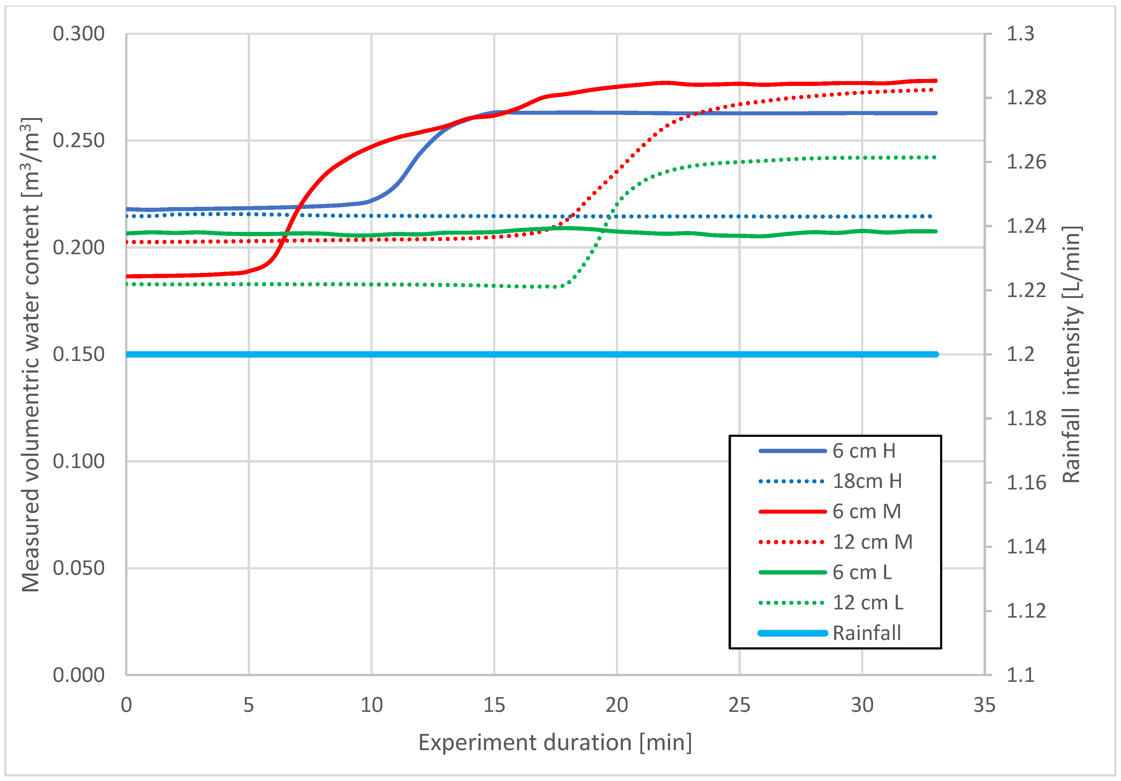
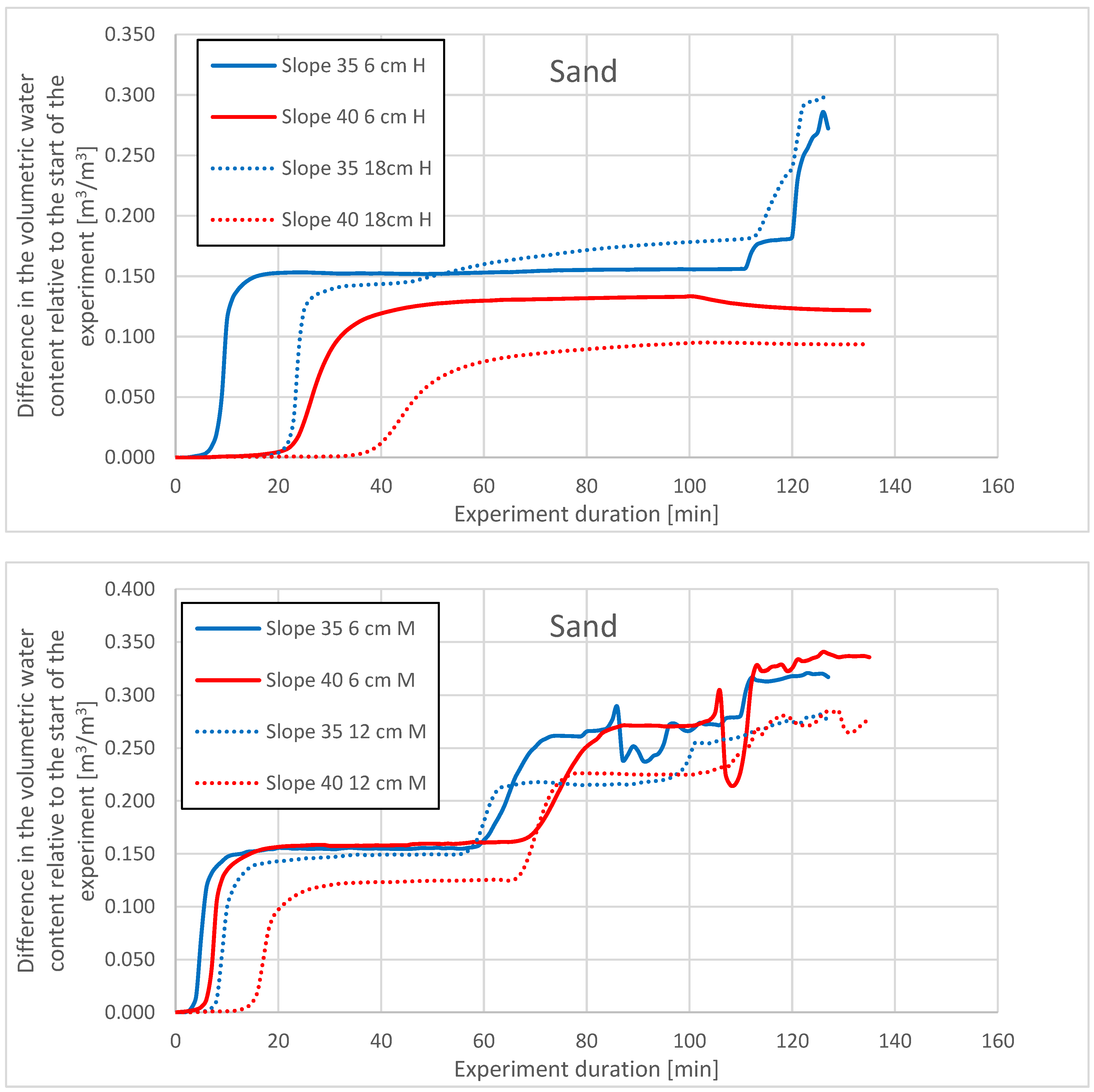
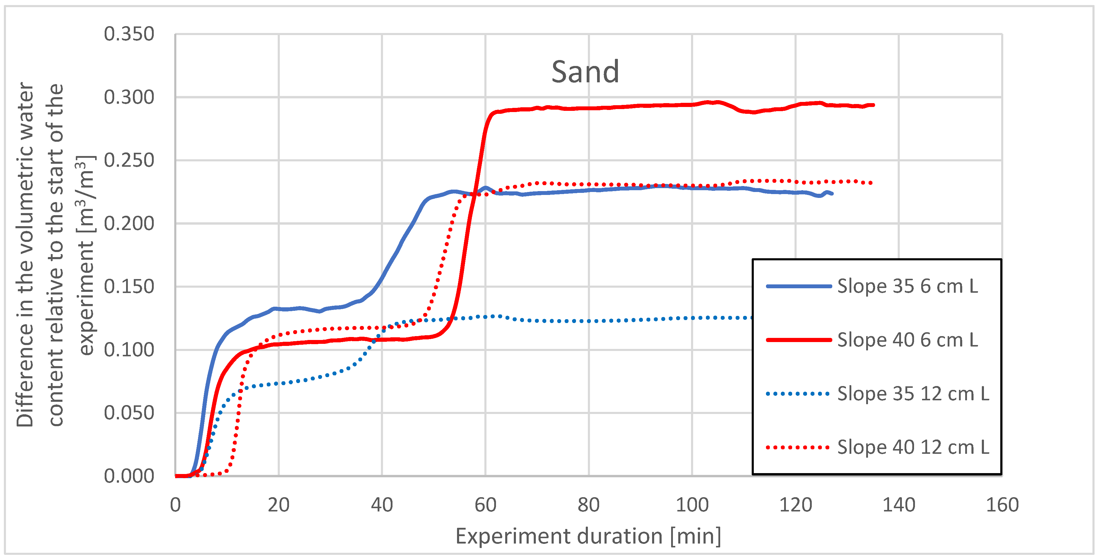
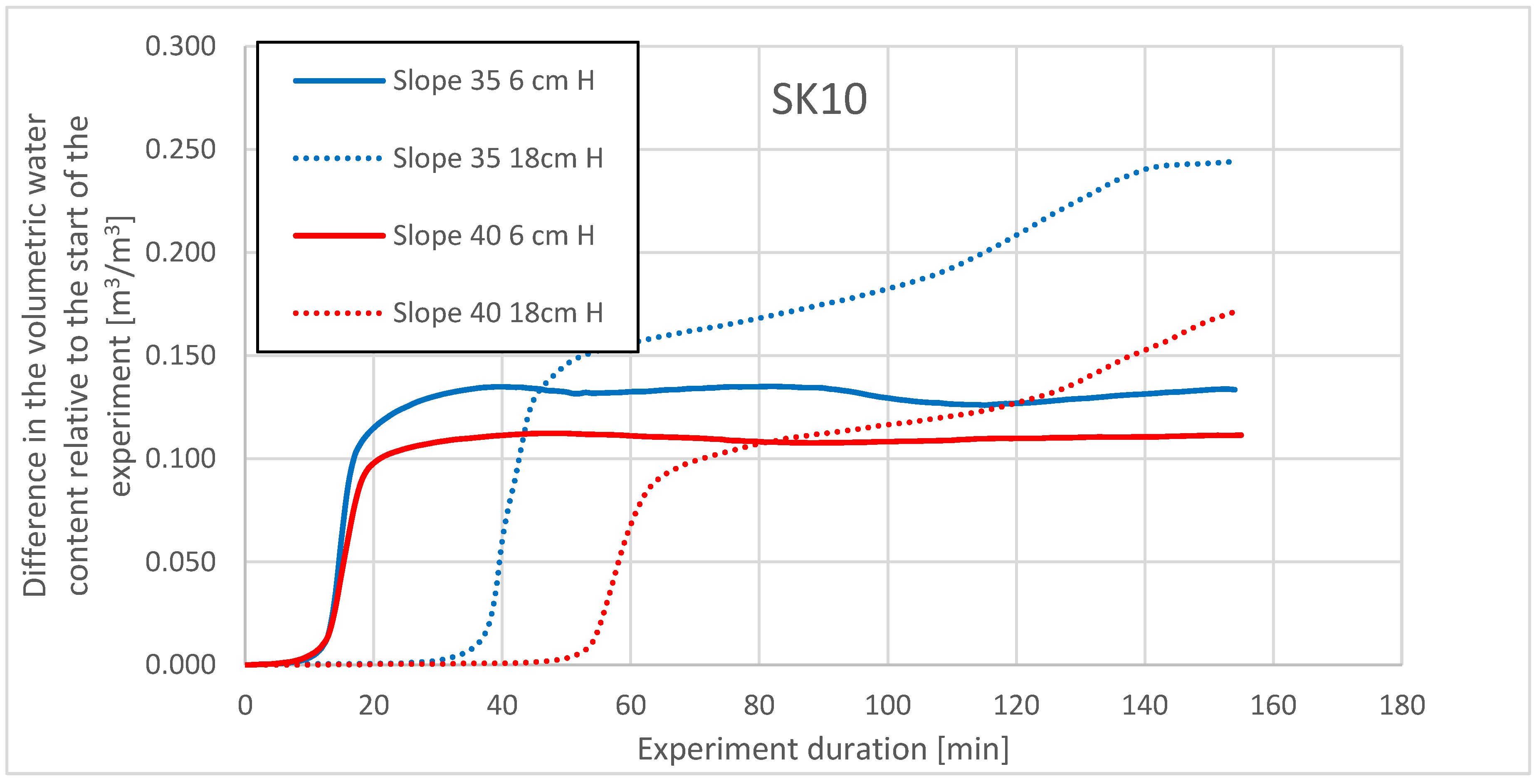
Additionally, we also compared changes in the volumetric water content for different experiments (Section 2.4). Since the initial volumetric moisture was not completely the same at all locations in the experimental model (Table 2), we compared the relative change in the volumetric water content among different experiments. In the case of sandy material, the initial volumetric water content was within the range of 0.05 and 0.1 m3/m3 at different locations. The same applies for the SK10 experiment. Figure 9 and Figure 10 show comparisons of the volumetric water content. It can be seen that in the upper part of the model (H part), the higher slope of the model is associated with a delayed increase in volumetric water content for both selected experiments in comparison to a lower slope (Figure 9 and Figure 10). Similar observations could be observed for the H and M sections of the model built in SK10 material—the higher slope is associated with a later increase in soil moisture throughout the experiment. In the case of a steeper slope, water moves more quickly to lower sections of the experimental model compared to a gentler slope. A similar impact of slope inclination can be seen for the middle part (M) of the model as well (Figure 9 and Figure 10). In the case of sandy and SK10 material, there are some steep changes in the volumetric water content in the second part of the experiment that can be attributed to the formation of cracks and slips (Figure 9 and Figure 10). Similar behavior was also observed in some other studies [36]. In the lower part of the model, the situation is more complex and is a result of direct simulated rainfall on the top of the lower part, as well as the inflow of infiltrated water from the upper and middle parts of the model. Hence, water ponding occurred in this part of the small-scale landslide model (e.g., Figure 4 and Figure 9).
4. Conclusions
This study evaluates the performance of five selected rainfall loss methods from the perspective of reproducing the experimental laboratory results that were obtained using a small-scale landslide model with a variable slope inclination. Based on the results presented, several important conclusions can be made:
- For some laboratory experiments, the initial rainfall loss method parameters estimated based on the literature provided a relatively good approximation of the experimental results in terms of the occurrence of surface runoff and its timing. In some other cases (SK10er), however, the rainfall–runoff model simulations using initial parameters yielded quite different results from those observed in the laboratory.
- The study results illustrate the importance of model calibration, even in cases where the slope material is homogenous and the material characteristics are well known (the uncertainty in parameter estimation is lower). Hence, it is essential to calibrate the rainfall loss method parameters in order to obtain adequate simulation results. It should be noted that, in some cases, the calibrated parameters differ significantly from the initial model parameters and, to some extent, also from the values that can be derived from the literature.
- None of the tested rainfall loss methods could be declared as a superior one and the performance of the tested methods depends on the specific characteristics of the laboratory experiment. Only in one case (SK10er experiment), for one of the methods, the parameters could not be changed in any way to reproduce the experimental results (calibration was not possible). In all other cases, post-experimental model calibration was successful.
- A comparison of the changes in volumetric water content as a function of slope and material characteristics (Sand and SK10) indicates that, in both cases, similar patterns could be detected for the upper and middle parts of the model, and that the model slope has a relatively significant impact on the changes in volumetric water content as a result of water movement within the model due to gravity effects (settlement of layers in the slope).
Compared to some of the previously conducted studies in which laboratory experiments with small-scale landslides were conducted to investigate slope stability, failure mechanisms and landslide dynamics, this study evaluates the performance of five rainfall loss methods for simulating the surface runoff during the experiments. It is recommended that rainfall loss methods are further tested using existing laboratory results on small-scale landslide models from other studies to gain further insights into the landslide hydrology at a small (laboratory) scale, as well as hillslope hydrology for the initiation of rainfall-induced landslides.
Author Contributions
Conceptualization, N.B. and J.P.; methodology, N.B.; formal analysis, N.B. and J.P.; investigation, J.P. and Ž.A.; data curation, J.P. and Ž.A.; writing—original draft preparation, N.B.; writing—review and editing, J.P., M.M. and Ž.A. All authors have read and agreed to the published version of the manuscript.
Funding
The software and research activities were supported by the Croatian Science Foundation under the project IP-2018-01-1503, “Physical modelling of landslide remediation constructions behaviour under static and seismic actions (ModLandRemSS)”. N. Bezak and M. Mikoš would like to acknowledge support from the Slovenian Research Agency (ARRS) through grants P2-0180 and V2-2137 and work conducted within the scope of the UNESCO Chair on Water-Related Disaster Risk Reduction.
Institutional Review Board Statement
Not applicable.
Informed Consent Statement
Not applicable.
Data Availability Statement
Data available on request.
Acknowledgments
We would like to thank the support staff from the University of Rijeka who were involved in conducting the laboratory experiments. Critical and useful comments from two anonymous reviewers greatly improved this work.
Conflicts of Interest
The authors declare no conflict of interest.
References
- Mikoš, M. After 2000 Stože landslide: Part II—Development in landslide disaster risk reduction policy in Slovenia—Po zemeljskem plazu Stože leta 2000: Del II—Razvoj politike zmanjševanja tveganja nesreč zaradi zemeljskih plazov v Sloveniji. Acta Hydrotech. 2021, 34, 39–59. [Google Scholar] [CrossRef]
- Mikoš, M. After 2000 Stože landslide: Part I—Development in landslide research in Slovenia—Po zemeljskem plazu Stože leta 2000: Del I—Razvoj raziskovanja zemeljskih plazov v Sloveniji. Acta Hydrotech. 2020, 33, 129–153. [Google Scholar] [CrossRef]
- Mikoš, M. Flood hazard in Slovenia and assessment of extreme design floods—Poplavna nevarnost v sloveniji in ocena ekstremnih projektnih poplavnih pretokov. Acta Hydrotech. 2020, 33, 43–59. [Google Scholar] [CrossRef]
- Islam, M.A.; Islam, M.S.; Chowdhury, M.E.; Badhon, F.F. Influence of vetiver grass (Chrysopogon zizanioides) on infiltration and erosion control of hill slopes under simulated extreme rainfall condition in Bangladesh. Arab. J. Geosci. 2021, 14, 119. [Google Scholar] [CrossRef]
- Islam, M.S.; Azijul Islam, M. Reduction of Landslide Risk and Water-Logging Using Vegetation. E3S Web Conf. 2018, 65, 06003. [Google Scholar] [CrossRef]
- Jelen, M.; Mikoš, M.; Bezak, N. Karst springs in Slovenia: Trend analysis—Kraški izviri v Sloveniji: Analiza trendov. Acta Hydrotech. 2020, 33, 1–12. [Google Scholar] [CrossRef]
- Sidle, R.C.; Greco, R.; Bogaard, T. Overview of Landslide Hydrology. Water 2019, 11, 148. [Google Scholar] [CrossRef]
- Šraj, M.; Dirnbek, L.; Brilly, M. The influence of effective rainfall on modeled runoff hydrograph|Vplyv efekťvnych zrážok na modelovaný hydrograf odtoku. J. Hydrol. Hydromech. 2010, 58, 3–14. [Google Scholar] [CrossRef]
- HEC HMS. HEC HMS User’s Manual, v. 4.7; US Army Corps of Engineers: Davis, CA, USA, 2021.
- Štajdohar, M.; Brilly, M.; Šraj, M. The influence of sustainable measures on runoff hydrograph from an urbanized drainage area. Acta Hydrotech. 2016, 29, 145–162. [Google Scholar]
- Sapač, K.; Medved, A.; Rusjan, S.; Bezak, N. Investigation of low- and high-flow characteristics of karst catchments under climate change. Water 2019, 11, 925. [Google Scholar] [CrossRef]
- Sezen, C.; Šraj, M.; Medved, A.; Bezak, N. Investigation of rain-on-snow floods under climate change. Appl. Sci. 2020, 10, 1242. [Google Scholar] [CrossRef] [Green Version]
- Bezak, N.; Petan, S.; Kobold, M.; Brilly, M.; Bálint, Z.; Balabanova, S.; Cazac, V.; Csík, A.; Godina, R.; Janál, P.; et al. A catalogue of the flood forecasting practices in the Danube River Basin. River Res. Appl. 2021, 37, 909–918. [Google Scholar] [CrossRef]
- Bezak, N.; Kovačević, M.; Johnen, G.; Lebar, K.; Zupanc, V.; Vidmar, A.; Rusjan, S. Exploring options for flood risk management with special focus on retention reservoirs. Sustainability 2021, 13, 10099. [Google Scholar] [CrossRef]
- Sezen, C.; Bezak, N.; Šraj, M. Hydrological modelling of the karst Ljubljanica River catchment using lumped conceptual model. Acta Hydrotech. 2018, 31, 87–100. [Google Scholar] [CrossRef]
- Addor, N.; Melsen, L.A. Legacy, Rather Than Adequacy, Drives the Selection of Hydrological Models. Water Resour. Res. 2019, 55, 378–390. [Google Scholar] [CrossRef]
- Astagneau, P.C.; Thirel, G.; Delaigue, O.; Guillaume, J.H.A.; Parajka, J.; Brauer, C.C.; Viglione, A.; Buytaert, W.; Beven, K.J. Technical note: Hydrology modelling R packages—A unified analysis of models and practicalities from a user perspective. Hydrol. Earth Syst. Sci. 2021, 25, 3937–3973. [Google Scholar] [CrossRef]
- Bai, Y.; Bezak, N.; Sapač, K.; Klun, M.; Zhang, J. Short-Term Streamflow Forecasting Using the Feature-Enhanced Regression Model. Water Resour. Manag. 2019, 33, 4783–4797. [Google Scholar] [CrossRef]
- Bezak, N.; Sodnik, J.; Maček, M.; Jurček, T.; Jež, J.; Peternel, T.; Mikoš, M. Investigation of potential debris flows above the Koroška Bela settlement, NW Slovenia, from hydro-technical and conceptual design perspectives. Landslides 2021, 18, 3891–3906. [Google Scholar] [CrossRef]
- Bezak, N.; Mikoš, M.; Šraj, M. Development of the methodology for the design hydrograph estimation. In Proceedings of the Mišičev Vodarski Dan; VGP Maribor: Maribor, Slovenija, 2021; pp. 50–58. [Google Scholar]
- Delleur, J. The Handbook of Groundwater Engineering; CRC Press: Boca Raton, FL, USA, 1999; ISBN 0-8493-2698-2. [Google Scholar]
- Halwatura, D.; Najim, M.M.M. Application of the HEC-HMS model for runoff simulation in a tropical catchment. Environ. Model. Softw. 2013, 46, 155–162. [Google Scholar] [CrossRef]
- Zema, D.A.; Labate, A.; Martino, D.; Zimbone, S.M. Comparing Different Infiltration Methods of the HEC-HMS Model: The Case Study of the Mésima Torrent (Southern Italy). L. Degrad. Dev. 2017, 28, 294–308. [Google Scholar] [CrossRef]
- Ceola, S.; Arheimer, B.; Baratti, E.; Blöschl, G.; Capell, R.; Castellarin, A.; Freer, J.; Han, D.; Hrachowitz, M.; Hundecha, Y.; et al. Virtual laboratories: New opportunities for collaborative water science. Hydrol. Earth Syst. Sci. 2015, 19, 2101–2117. [Google Scholar] [CrossRef] [Green Version]
- Blöschl, G.; Blaschke, A.P.; Broer, M.; Bucher, C.; Carr, G.; Chen, X.; Eder, A.; Exner-Kittridge, M.; Farnleitner, A.; Flores-Orozco, A.; et al. The Hydrological Open Air Laboratory (HOAL) in Petzenkirchen: A hypothesis-driven observatory. Hydrol. Earth Syst. Sci. 2016, 20, 227–255. [Google Scholar] [CrossRef]
- Sapač, K.; Bezak, N.; Vidmar, A.; Rusjan, S. Nitrate nitrogen (no3-n) export regimes based on high-frequency measurements in the kuzlovec stream catchment|Režimi iznosov nitratnega dušika (no3-n) na podlagi meritev s kratkim časovnim korakom na porečju vodotoka kuzlovec. Acta Hydrotech. 2021, 34, 25–38. [Google Scholar] [CrossRef]
- Ferreira, C.S.S.; Keizer, J.J.; Santos, L.M.B.; Serpa, D.; Silva, V.; Cerqueira, M.; Ferreira, A.J.D.; Abrantes, N. Runoff, sediment and nutrient exports from a Mediterranean vineyard under integrated production: An experiment at plot scale. Agric. Ecosyst. Environ. 2018, 256, 184–193. [Google Scholar] [CrossRef]
- Song, J.; Wang, J.; Wang, W.; Peng, L.; Li, H.; Zhang, C.; Fang, X. Comparison between different infiltration models to describe the infiltration of permeable brick pavement system via a laboratory-scale experiment. Water Sci. Technol. 2021, 84, 2214–2227. [Google Scholar] [CrossRef]
- Haowen, X.; Yawen, W.; Luping, W.; Weilin, L.; Wenqi, Z.; Hong, Z.; Yichen, Y.; Jun, L. Comparing simulations of green roof hydrological processes by SWMM and HYDRUS-1D. Water Sci. Technol. Water Supply 2020, 20, 130–139. [Google Scholar] [CrossRef]
- Gu, W.-Z.; Liu, J.-F.; Lin, H.; Lin, J.; Liu, H.-W.; Liao, A.-M.; Wang, N.; Wang, W.-Z.; Ma, T.; Yang, N.; et al. Why hydrological maze: The hydropedological trigger? Review of experiments at Chuzhou hydrology laboratory. Vadose Zone J. 2018, 17, 170174. [Google Scholar] [CrossRef]
- Pajalić, S.; Peranić, J.; Maksimović, S.; Čeh, N.; Jagodnik, V.; Arbanas, Ž. Monitoring and Data Analysis in Small-Scale Landslide Physical Model. Appl. Sci. 2021, 11, 5040. [Google Scholar] [CrossRef]
- Jagodnik, V.; Peranić, J.; Arbanas, Ž. Mechanism of Landslide Initiation in Small-Scale Sandy Slope Triggered by an Artificial Rain. In Understanding and Reducing Landslide Disaster Risk: Volume 6 Specific Topics in Landslide Science and Applications; Arbanas, Ž., Bobrowsky, P.T., Konagai, K., Sassa, K., Takara, K., Eds.; Springer International Publishing: Cham, Switzerland, 2021; pp. 177–184. ISBN 978-3-030-60713-5. [Google Scholar]
- Huang, A.-B.; Lee, J.-T.; Ho, Y.-T.; Chiu, Y.-F.; Cheng, S.-Y. Stability monitoring of rainfall-induced deep landslides through pore pressure profile measurements. Soils Found. 2012, 52, 737–747. [Google Scholar] [CrossRef]
- Hungr, O.; Morgenstern, N.R. Experiments on the flow behaviour of granular materials at high velocity in an open channel. Geotechnique 1984, 34, 405–413. [Google Scholar] [CrossRef]
- Wu, L.Z.; Zhou, Y.; Sun, P.; Shi, J.S.; Liu, G.G.; Bai, L.Y. Laboratory characterization of rainfall-induced loess slope failure. CATENA 2017, 150, 1–8. [Google Scholar] [CrossRef]
- Spolverino, G.; Capparelli, G.; Versace, P. An Instrumented Flume for Infiltration Process Modeling, Landslide Triggering and Propagation. Geosciences 2019, 9, 108. [Google Scholar] [CrossRef]
- Capparelli, G.; Damiano, E.; Greco, R.; Olivares, L.; Spolverino, G. Physical modeling investigation of rainfall infiltration in steep layered volcanoclastic slopes. J. Hydrol. 2020, 580, 124199. [Google Scholar] [CrossRef]
- Park, J.-Y.; Song, Y.-S. Laboratory Experiment and Numerical Analysis on the Precursory Hydraulic Process of Rainfall-Induced Slope Failure. Adv. Civ. Eng. 2020, 2020, 2717356. [Google Scholar] [CrossRef]
- Formetta, G.; Capparelli, G.; Versace, P. Evaluating performance of simplified physically based models for shallow landslide susceptibility. Hydrol. Earth Syst. Sci. 2016, 20, 4585–4603. [Google Scholar] [CrossRef]
- Krøgli, I.K.; Devoli, G.; Colleuille, H.; Boje, S.; Sund, M.; Engen, I.K.; Krogli, I.K.; Devoli, G.; Colleuille, H.; Boje, S.; et al. The Norwegian forecasting and warning service for rainfall- and snowmelt-induced landslides. Nat. Hazards Earth Syst. Sci. 2018, 18, 1427–1450. [Google Scholar] [CrossRef]
- Hong, Y.; Adler, R.F. Predicting global landslide spatiotemporal distribution: Integrating landslide susceptibility zoning techniques and real-time satellite rainfall estimates. Int. J. Sediment Res. 2008, 23, 249–257. [Google Scholar] [CrossRef]
- Hungr, O.; Leroueil, S.; Picarelli, L. The Varnes classification of landslide types, an update. Landslides 2014, 11, 167–194. [Google Scholar] [CrossRef]
- Dowling, C.A.; Santi, P.M. Debris flows and their toll on human life: A global analysis of debris-flow fatalities from 1950 to 2011. Nat. Hazards 2014, 71, 203–227. [Google Scholar] [CrossRef]
- Andres, N.; Badoux, A. The Swiss flood and landslide damage database: Normalisation and trends. J. Flood Risk Manag. 2019, 12, e12510. [Google Scholar] [CrossRef]
- Gariano, S.L.; Guzzetti, F. Landslides in a changing climate. Earth-Sci. Rev. 2016, 162, 227–252. [Google Scholar] [CrossRef] [Green Version]
- Jemec Auflič, M.; Bokal, G.; Kumelj, Š.; Medved, A.; Dolinar, M.; Jež, J. Impact of climate change on landslides in Slovenia in the mid-21st century. Geologija 2021, 64, 159–171. [Google Scholar] [CrossRef]
- Gariano, S.L.; Rianna, G.; Petrucci, O.; Guzzetti, F. Assessing future changes in the occurrence of rainfall-induced landslides at a regional scale. Sci. Total Environ. 2017, 596–597, 417–426. [Google Scholar] [CrossRef] [PubMed]
- Bezak, N.; Mikoš, M. Changes in the rainfall event characteristics above the empirical global rainfall thresholds for landslide initiation at the pan-European level. Landslides 2021, 18, 1859–1873. [Google Scholar] [CrossRef]
- Vivoda Prodan, M.; Peranić, J.; Pajalić, S.; Jagodnik, V.; Čeh, N.; Arbanas, Ž. Mechanism of rainfall induced landslides in small-scale models built of different materials. In Proceedings of the 5th Regional Symposium on Landslides in Adriatic-Balkan Region; Peranić, J., Vivoda Prodan, M., Bernat Gazibara, S., Krkač, M., Mihalić Arbanas, S., Arbanas, Ž., Eds.; University of Rijeka: Rijeka, Croatia, 2022. [Google Scholar]
- Peranić, J.; Jagodnik, V.; Čeh, N.; Vivoda Prodan, M.; Pajalić, S.; Arbanas, Ž. Small-scale physical landslide models under 1g infiltration conditions and the role of hydrological monitoring. In Proceedings of the 5th Regional Symposium on Landslides in Adriatic-Balkan Region; Peranić, J., Vivoda Prodan, M., Bernat Gazibara, S., Krkač, M., Mihalić Arbanas, S., Arbanas, Ž., Eds.; University of Rijeka: Rijeka, Croatia, 2022. [Google Scholar]
- Arbanas, Ž.; Peranić, J.; Jagodnik, V.; Vivoda Prodan, M.; Čeh, N.; Pajalić, S.; Plazonić, D. Impact of gravity retaining wall on the stability of a sandy slope in small-scale physical model. In Proceedings of the 5th Regional Symposium on Landslides in Adriatic-Balkan Region; Peranić, J., Vivoda Prodan, M., Bernat Gazibara, S., Krkač, M., Mihalić Arbanas, S., Arbanas, Ž., Eds.; University of Rijeka: Rijeka, Croatia, 2022. [Google Scholar]
- Mein, R.G.; Larson, C.L. Modeling infiltration during a steady rain. Water Resour. Res. 1973, 9, 384–394. [Google Scholar] [CrossRef]
- Heber Green, W.; Ampt, G.A. Studies on Soil Phyics. J. Agric. Sci. 1911, 4, 1–24. [Google Scholar] [CrossRef]
- Richards, L.A. Capillary conduction of liquids through porous mediums. Physics 1931, 1, 318–333. [Google Scholar] [CrossRef]
- Rawls, W.J.; Gish, T.J.; Brakensiek, D.L. Estimating Soil Water Retention from Soil Physical Properties and Characteristics. In Advances in Soil Science: Volume 16; Stewart, B.A., Ed.; Springer: New York, NY, USA, 1991; pp. 213–234. ISBN 978-1-4612-3144-8. [Google Scholar]
- Banasik, K.; Rutkowska, A.; Kohnová, S. Retention and curve number variability in a small agricultural catchment: The probabilistic approach. Water 2014, 6, 1118–1133. [Google Scholar] [CrossRef]
- Rutkowska, A.; Kohnová, S.; Banasik, K.; Szolgay, J.; Karabová, B. Probabilistic properties of a curve number: A case study for small Polish and Slovak Carpathian Basins. J. Mt. Sci. 2015, 12, 533–548. [Google Scholar] [CrossRef]
- Beven, K. The era of infiltration. Hydrol. Earth Syst. Sci. 2021, 25, 851–866. [Google Scholar] [CrossRef]
- Beven, K.; Robert, E. Horton’s perceptual model of infiltration processes. Hydrol. Process. 2004, 18, 3447–3460. [Google Scholar] [CrossRef]
- Akan, O.A. Urban Stormwater Hydrology: A Guide to Engineering Calculations, 1st ed.; CRC Press: Boca Raton, FL, USA, 1993; ISBN 0877629676. [Google Scholar]
- Lavtar, K.; Bezak, N.; Šraj, M. Rainfall-runoff modeling of the nested non-homogeneous sava river sub-catchments in Slovenia. Water 2020, 12, 128. [Google Scholar] [CrossRef]
- Garklavs, G.; Oberg, K.A. Effect of rainfall excess calculations on modeled hydrograph accuracy and unit-hydrograph parameters. JAWRA J. Am. Water Resour. Assoc. 1986, 22, 565–572. [Google Scholar] [CrossRef]
- Bezak, N.; Šraj, M.; Rusjan, S.; Mikoš, M. Impact of the rainfall duration and temporal rainfall distribution defined using the Huff curves on the hydraulic flood modelling results. Geosciences 2018, 8, 69. [Google Scholar] [CrossRef] [Green Version]
Figure 1.
A photo of the small-scale landslide model with a gabion wall applied as a remediation measure at the slope toe and with the indication of the main model elements.
Figure 1.
A photo of the small-scale landslide model with a gabion wall applied as a remediation measure at the slope toe and with the indication of the main model elements.

Figure 2.
A cross-section of the model with 30° slope (inclination) with the indication of the main geometric characteristics, soil moisture sensors’ positions (blue labels) and sprinkler branches in the upper (H), middle (M) and lower (L) parts of the model. Model dimensions are in meters.
Figure 2.
A cross-section of the model with 30° slope (inclination) with the indication of the main geometric characteristics, soil moisture sensors’ positions (blue labels) and sprinkler branches in the upper (H), middle (M) and lower (L) parts of the model. Model dimensions are in meters.

Figure 3.
Measured volumetric water content during the experiment with sand (Sand). Measured locations (H, M and L) are shown in Figure 2. Note that quick changes in the volumetric water content can be associated with the development of slope instabilities.
Figure 3.
Measured volumetric water content during the experiment with sand (Sand). Measured locations (H, M and L) are shown in Figure 2. Note that quick changes in the volumetric water content can be associated with the development of slope instabilities.

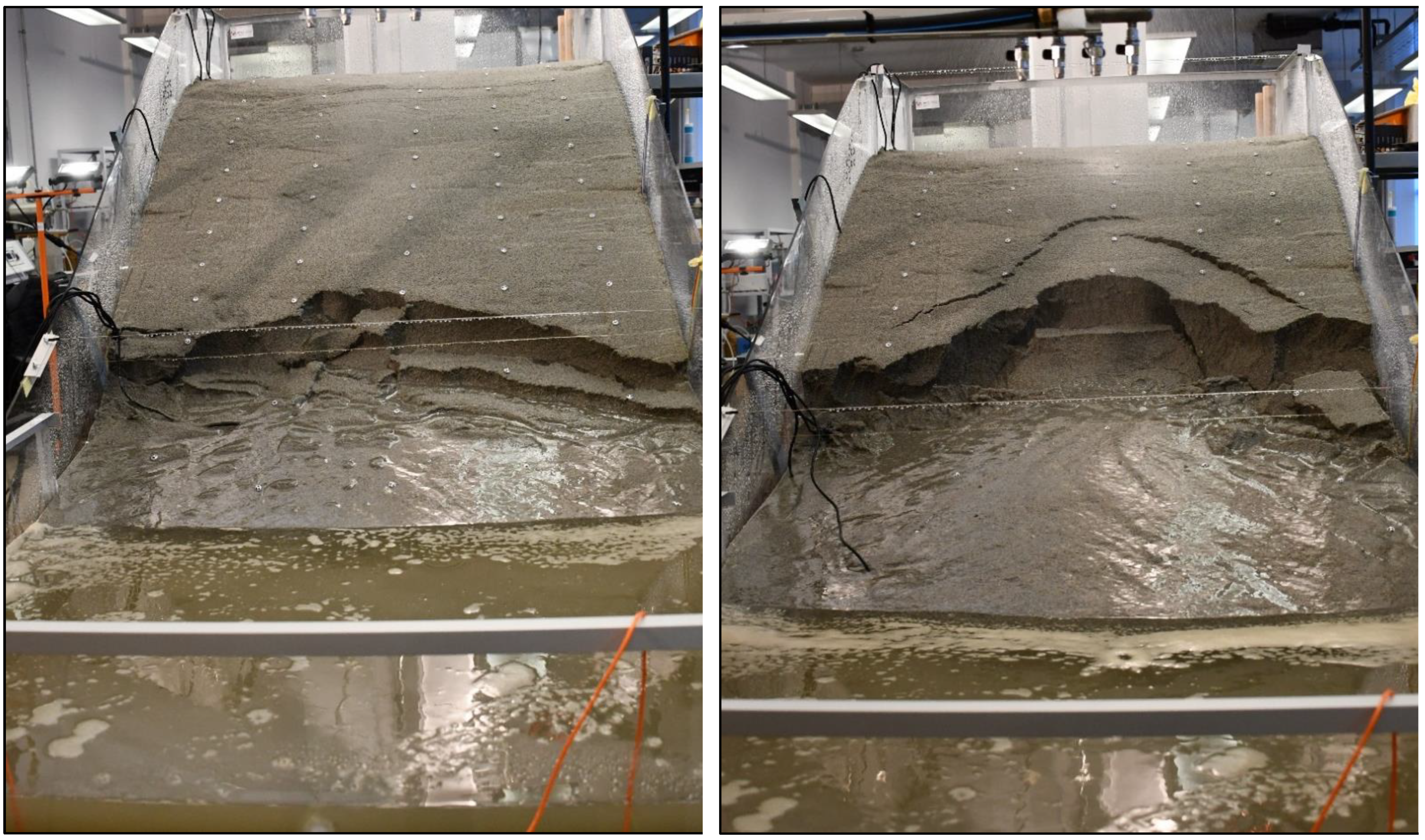
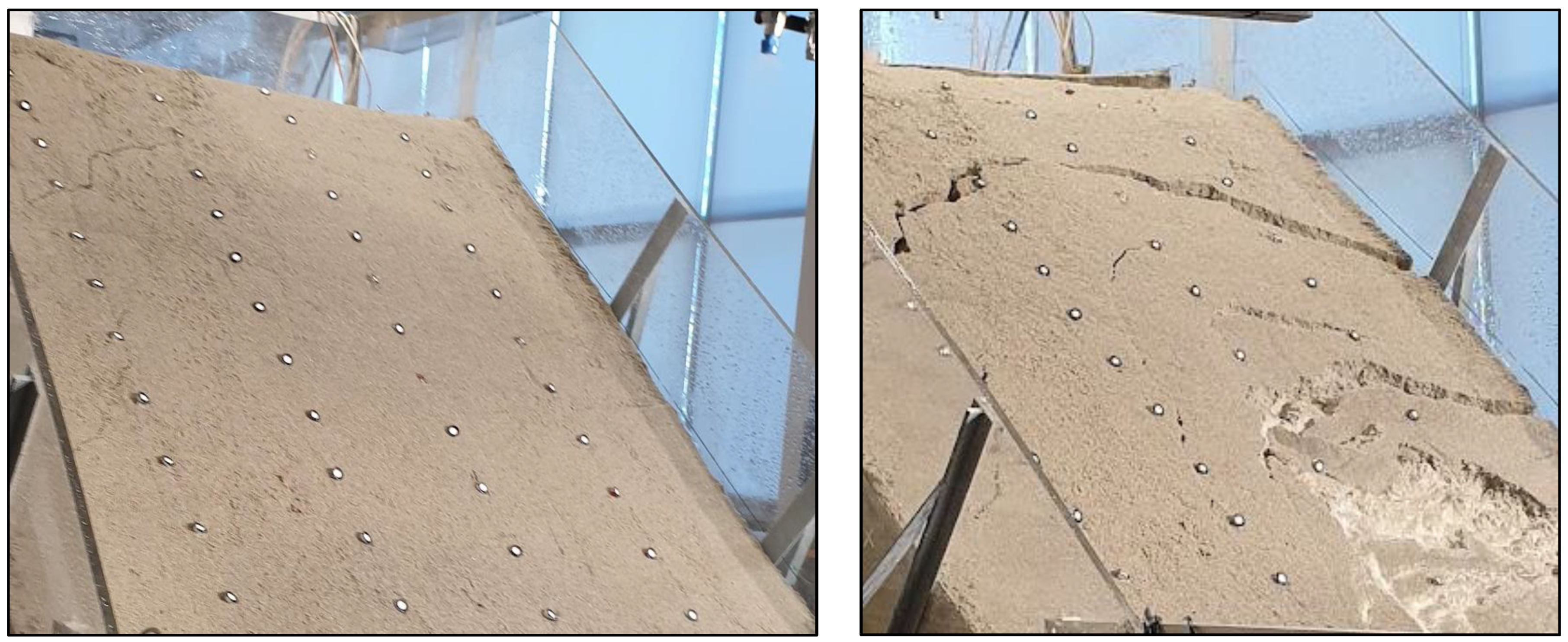
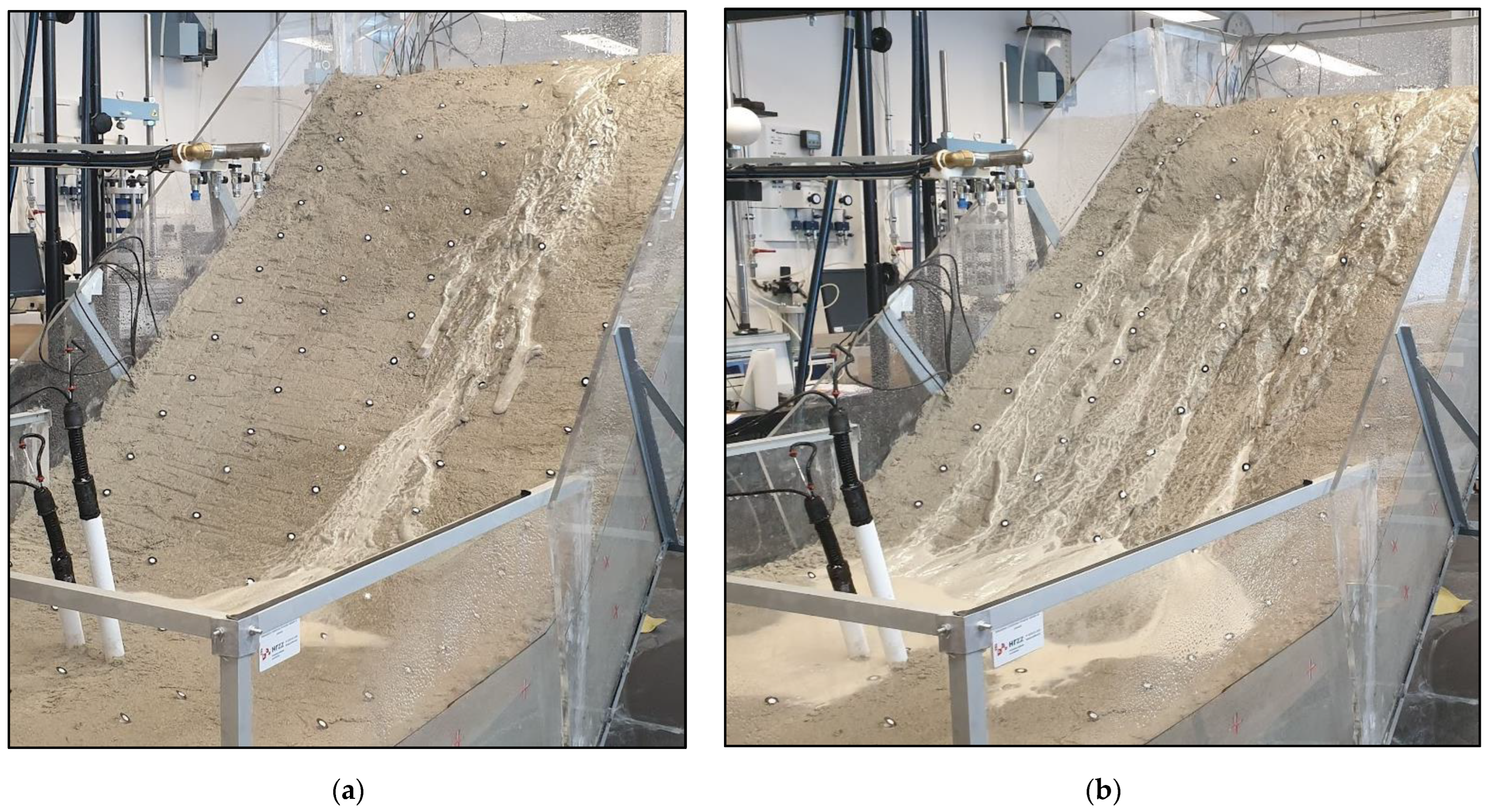
Figure 4.
A photo of the Sand experiment around 90 min after the start of the rainfall simulation (left), showing the evolution of the retrogressive sliding following the formation of the rotational slide in the slope’s toe, and a photo taken at the start of the surface runoff formation in the upper part of the model at around 125 min after the beginning of the Sand experiment (right).

Figure 5.
Measured volumetric water content during the SK10 experiment. Measured locations (H, M and L) are shown in Figure 2.
Figure 5.
Measured volumetric water content during the SK10 experiment. Measured locations (H, M and L) are shown in Figure 2.

Figure 6.
A photo of the second experiment considered (SK10) after around 55 min of the rainfall simulation, when first cracks were observed (left), and after 120 min (right), when further displacements took place, along with the mobilization of the large sliding surface in the model.
Figure 6.
A photo of the second experiment considered (SK10) after around 55 min of the rainfall simulation, when first cracks were observed (left), and after 120 min (right), when further displacements took place, along with the mobilization of the large sliding surface in the model.

Figure 7.
Measured volumetric water content during the SK10er experiment. Measured locations (H, M and L) are shown in Figure 2.
Figure 7.
Measured volumetric water content during the SK10er experiment. Measured locations (H, M and L) are shown in Figure 2.

Figure 8.
A photo of the SK10er experiment at around 8 (left) and 18 (right) min after the start of the experiment.
Figure 8.
A photo of the SK10er experiment at around 8 (left) and 18 (right) min after the start of the experiment.

Figure 9.
Comparison of the changes in the volumetric water content at different parts of the experimental model for the Sand experiment. Locations of measurement points are shown in Figure 2.
Figure 9.
Comparison of the changes in the volumetric water content at different parts of the experimental model for the Sand experiment. Locations of measurement points are shown in Figure 2.


Figure 10.
Comparison of the changes in the volumetric water content at different parts of the experimental model for the SK10 experiment. Locations of measurement points are shown in Figure 2.
Figure 10.
Comparison of the changes in the volumetric water content at different parts of the experimental model for the SK10 experiment. Locations of measurement points are shown in Figure 2.


Table 1.
Main characteristics of the slope material that was used for simulations. Adopted from Vivoda Prodan et al. [49].
Table 1.
Main characteristics of the slope material that was used for simulations. Adopted from Vivoda Prodan et al. [49].
| Slope Material | Sand | Sand–Kaolin (10%) | Sand–Kaolin (15%) |
|---|---|---|---|
| Specific gravity, Gs (/) | 2.70 | 2.69 | 2.67 |
| D10 (mm) | 0.190 | 0.038 | 0.056 |
| D60 (mm) | 0.370 | 0.310 | 0.207 |
| Uniformity coefficient, cu (/) | 1.95 | 8.16 | 54.11 |
| Minimum void ratio, emin (/) | 0.64 | 0.65 | 0.54 |
| Maximum void ratio, emax (/) | 0.91 | 1.21 | 1.43 |
| Hydraulic conductivity, ks (m/s) | 1.0 × 10⁻⁵ | 6.8 × 10⁻⁶ | 3.5 × 10⁻⁶ |
| Friction angle, ϕ (◦) | 34.9 | 31.3 | 31.8 |
| Cohesion, c (kPa) | 0 | 3.9 | 4.4 |
| Targeted initial porosity, ni (/) | 0.44 | 0.47 | 0.43 |
| Targeted initial relative density, Dr (/) | 0.5 | 0.5 | 0.75 |
| Targeted initial water content, wi (%) | 2 | 5 | 8.1 |
Table 2.
Green and Ampt initial parameters that were used for the rainfall–runoff simulations.
| Parameter/Experiment | Sand | SK10 | SK10er |
|---|---|---|---|
| Initial Content (m3/m3) | 0.06 | 0.09 | 0.22 |
| Saturated Content (m3/m3) | 0.44 | 0.47 | 0.47 |
| Suction (mm) | 50 | 100 | 100 |
| Conductivity (mm/h) | 36 | 25 | 25 |
Table 3.
Smith Parlange initial parameters that were used for the rainfall–runoff simulations.
| Parameter/Experiment | Sand | SK10 | SK10er |
|---|---|---|---|
| Initial Content (m3/m3) | 0.06 | 0.09 | 0.22 |
| Residual Content (m3/m3) | 0.02 | 0.02 | 0.02 |
| Saturated Content (m3/m3) | 0.44 | 0.47 | 0.47 |
| Bubbling Pressure (mm) | 50 | 100 | 100 |
| Pore Distribution | 0.6 | 0.5 | 0.5 |
| Conductivity (mm/h) | 36 | 25 | 25 |
Table 4.
Initial and constant method initial parameters that were used for the rainfall–runoff simulations.
Table 4.
Initial and constant method initial parameters that were used for the rainfall–runoff simulations.
| Parameter/Experiment | Sand | SK10 | SK10er |
|---|---|---|---|
| Initial Loss (mm) | 114 | 114 | 60 |
| Constant Rate (mm/h) | 36 | 25 | 25 |
Table 5.
Horton infiltration method initial parameters that were used for the rainfall–runoff simulations.
Table 5.
Horton infiltration method initial parameters that were used for the rainfall–runoff simulations.
| Parameter/Experiment | Sand | SK10 | SK10er |
|---|---|---|---|
| k (1/h) | 2 | 2 | 2 |
| f0 (mm/h) | 127 | 76 | 76 |
| fc (mm/h) | 10 | 9 | 9 |
Table 6.
Ranking-based performance metrics of different tested rainfall loss methods according to the methodology shown in Section 2.3. Values outside and inside brackets indicate performance with initial model parameters and after manual calibration, respectively.
Table 6.
Ranking-based performance metrics of different tested rainfall loss methods according to the methodology shown in Section 2.3. Values outside and inside brackets indicate performance with initial model parameters and after manual calibration, respectively.
| Method/Experiment | Sand | SK10 | SK10er |
|---|---|---|---|
| Green and Ampt | 2 (3) | 3 (3) | 1 (3) |
| Smith Parlange | 2 (3) | 3 (3) | 1 (3) |
| Initial and Constant | 3 (3) | 3 (3) | 1 (3) |
| SCS Curve Number | 2 (3) | 1 (3) | 3 (3) |
| Horton Infiltration | 2 (3) | 0 (3) | 1 (1) |
Table 7.
Calibrated values of parameters for different experiments using the Green and Ampt method. Initial values are shown in Table 2.
Table 7.
Calibrated values of parameters for different experiments using the Green and Ampt method. Initial values are shown in Table 2.
| Parameter/Experiment | Sand | SK10 | SK10er |
|---|---|---|---|
| Initial Content (m3/m3) | 0.06 | 0.09 | 0.22 |
| Saturated Content (m3/m3) | 0.44 | 0.47 | 0.47 |
| Suction (mm) | 50 | 100 | 40 |
| Conductivity (mm/h) | 60 | 25 | 10 |
Table 8.
Calibrated values of parameters for different experiments using the Smith Parlange method. Initial values are shown in Table 3.
Table 8.
Calibrated values of parameters for different experiments using the Smith Parlange method. Initial values are shown in Table 3.
| Parameter/Experiment | Sand | SK10 | SK10er |
|---|---|---|---|
| Initial Content (m3/m3) | 0.06 | 0.09 | 0.22 |
| Residual Content (m3/m3) | 0.02 | 0.02 | 0.02 |
| Saturated Content (m3/m3) | 0.44 | 0.47 | 0.47 |
| Bubbling Pressure (mm) | 50 | 100 | 40 |
| Pore Distribution | 0.44 | 0.5 | 0.47 |
| Conductivity (mm/h) | 69 | 25 | 10 |
Table 9.
Calibrated values of parameters for different experiments using the initial and constant method. Initial values are shown in Table 4.
Table 9.
Calibrated values of parameters for different experiments using the initial and constant method. Initial values are shown in Table 4.
| Parameter/Experiment | Sand | SK10 | SK10er |
|---|---|---|---|
| Initial Loss (mm) | 114 | 80 | 8 |
| Constant Rate (mm/h) | 36 | 25 | 10 |
Table 10.
Initial and calibrated values of parameters for different experiments using the SCS curve number method.
Table 10.
Initial and calibrated values of parameters for different experiments using the SCS curve number method.
| SCS Curve Number | Sand | SK10 | SK10er |
|---|---|---|---|
| Initial parameters | 77 | 86 | 86 |
| Calibrated parameters | 32 | 38 | 86 |
Table 11.
Calibrated values of parameters for different experiments using the Horton method. Initial values are shown in Table 5.
Table 11.
Calibrated values of parameters for different experiments using the Horton method. Initial values are shown in Table 5.
| Parameter/Experiment | Sand | SK10 | SK10er |
|---|---|---|---|
| k (1/h) | 2 | 2 | 2 |
| f0 (mm/h) | 220 | 80 | 76 |
| fc (mm/h) | 60 | 11 | 9 |
Publisher’s Note: MDPI stays neutral with regard to jurisdictional claims in published maps and institutional affiliations. |
© 2022 by the authors. Licensee MDPI, Basel, Switzerland. This article is an open access article distributed under the terms and conditions of the Creative Commons Attribution (CC BY) license (https://creativecommons.org/licenses/by/4.0/).
Share and Cite
MDPI and ACS Style
Bezak, N.; Peranić, J.; Mikoš, M.; Arbanas, Ž. Evaluation of Hydrological Rainfall Loss Methods Using Small-Scale Physical Landslide Model. Water 2022, 14, 2726. https://doi.org/10.3390/w14172726
AMA Style
Bezak N, Peranić J, Mikoš M, Arbanas Ž. Evaluation of Hydrological Rainfall Loss Methods Using Small-Scale Physical Landslide Model. Water. 2022; 14(17):2726. https://doi.org/10.3390/w14172726
Chicago/Turabian StyleBezak, Nejc, Josip Peranić, Matjaž Mikoš, and Željko Arbanas. 2022. "Evaluation of Hydrological Rainfall Loss Methods Using Small-Scale Physical Landslide Model" Water 14, no. 17: 2726. https://doi.org/10.3390/w14172726
Note that from the first issue of 2016, this journal uses article numbers instead of page numbers. See further details here.