In Situ Pumping–Injection Remediation of Strong Acid–High Salt Groundwater: Displacement–Neutralization Mechanism and Influence of Pore Blocking

Abstract

Acid-polluted groundwater may cause many environmental problems due to its corrosivity. Pumping and injection technology is a commonly used remediation technology, and its main principles are displacement and neutralization. However, due to the high salinity in groundwater, blockage easily occurs and reduces the efficiency. The mechanism of pumping and remediation of strong acid–high salinity groundwater is unclear, and the mechanism and effect of pore blocking are unknown. In this paper, based on an actual polluted site, a field pumping test was carried out. Through groundwater monitoring and drilling core sampling, the process and mechanism of acid groundwater pumping–injection remediation were clarified, and the principle and impact of pore blockage are revealed. The results showed that increasing the injection pressure can effectively improve the repairing efficiency. When the pressure increased from 0.2 MPa to 0.3 MPa, the water injection efficiency per unit time was increased by more than 20%. The principle of pumping–injection remediation of acidic groundwater was mainly displacement, accounting for more than 93%, while neutralization only contributed less than 0.1%. Although the neutralization contribution was small, the neutralization interface of injected alkaline water and acidic groundwater was the main place for precipitation. The precipitation was mainly formed around the injection well, the amount of which decreases greatly with the increase in displacement distance. This was because the formation of precipitation required both an appropriate concentration of Fe and high pH (5.63). Affected by neutralization and dispersion, the pH of the acid–base water interface decreased and the necessary conditions for the formation of precipitation were not met. Therefore, in the actual pumping–injection restoration project, optimization can be carried out from two perspectives of appropriately increasing the injected water pressure and reducing the injected water pH. This study has important reference value for the control and remediation of such acid-polluted groundwater.

1. Introduction

Pump-and-treat (PAT) is one of the most widely used remediation technologies for contaminated aquifers [1,2,3], mostly implemented for the remediation of groundwater polluted with high concentrations of soluble pollutants, which can be very effective for source removal and plume control [4,5,6,7]. In a typical PAT system, contaminated groundwater is pumped from the aquifer and treated above ground, then injected back into the aquifer or discharged [8,9,10]. By contrast, the traditional technology with only extraction, the pumping–injection technology with the addition of injection wells, has a higher displacement efficiency for pollutants [11].

Strong acid–high salt polluted groundwater is mostly caused by chemical weathering [12,13], acid leakage, discharge of acidic mine wastewater and chemical wastewater [14,15]. Acid groundwater pollution has been reported in the United States, South Korea, Australia, The Netherlands, etc. [16,17,18]. The Chemical Safety Clearing-house (CSC) system (https://CSC.me.go.kr, accessed on 7 August 2021), established by the Korean Ministry of Environment, reported that twenty-nine sulfuric acid leaks and eight hydrofluoric acid spills occurred between 2000 and 2018 [15]. In Australia, acid groundwater pollution caused by acidic soils is one of the major environmental and socio-economic problems [19]. Acid water enters the aquifer, increasing the dissolution of the aquifer medium that may significantly change the hydrogeological conditions [13], corrode aquiclude and cause cross-strata pollution, etc. The quality of the lower confined water is usually good and often used as a source of water supply; its pollution, therefore, may lead to greater environmental risks because its control and restoration is more difficult and costly. Therefore, increasing pH is the key to reducing the corrosiveness. Using the pumping–injection technology, injecting neutral or alkaline water combined with pumping for hydraulic control can achieve the purpose of rapidly increasing the pH of groundwater. However, acidic groundwater can dissolve minerals of the aqueous medium [20,21,22,23], resulting in a large amount of iron, aluminum, calcium, magnesium, etc. [15,24,25]. When the injected alkaline water contacts with the acid-polluted groundwater, the pH at the acid–base water interface rises rapidly, and the concentration of iron is also high, reaching the conditions for the formation of precipitation, which is easy-to-form iron oxide/hydroxide precipitation. The precipitation blocks the pores of the medium and reduces the permeability on account of the increased pH and high iron concentration [19,26]. It follows that when the pumping–injection technology is used to remediate acidic–high salt groundwater, it is easy to generate precipitation during the process of injecting alkaline water, reduce the permeability, decrease the effective influence radius and extend the repair time. From a summary of various studies, the causes of blockage can be summarized into three aspects. Firstly, hydrodynamic conditions, which is mainly the given water pressure during the water injection process [27,28]. Secondly, hydrochemical conditions, that is, differences in pH, iron concentration, etc., between injected water and polluted groundwater [29,30,31,32]. The last is the inherent permeability, particle size and porosity of the aqueous medium [33,34,35]. The increased injection pressure causes the higher hydraulic gradient, and the groundwater flow rate increases, resulting in a shorter residence time and less precipitation. At the same time, it can open up the water injection channel and increase the permeability, which will slow down the reduction in the water injection capacity caused by blockage. Differences in water quality between groundwater and injected water are also critical to the impact of injection. Previous studies have proposed the affinity theory between artificial recharge water and groundwater in aquifers, considered that injected water and original groundwater had good chemical affinity when chemical phases and soluble salt concentrations were similar and that the risk of problems, such as blockage and changes in water quality, was relatively small [29]. So, the chemical blockage usually formed by mineral precipitation mainly occurs in the front of the recharge water flow in the aquifer, that is, the mixed zone of groundwater and recharge water. For example, the blockage formed by iron precipitation often occurs near the infiltration zone [30]. The difference of the particle size and porosity of the aqueous medium has obvious influence on the blocking process and blocking degree [36,37]. For instance, in the injection of fine sand aquifers, the upper limit of the particulate matter content of the injection water quality was very low [37], while for sandy limestone aquifers with significant secondary pores, water with extremely high particulate matter content was continuously injected for 4 years [32]. Yan’s research showed that in the same area, different wells have different rock and soil particle sizes in aquifers; the recharge was also different, and the coarser the particles, the better the recharge effect [38]. Huang conducted a laboratory injection experiment on two kinds of sand samples with particle sizes of 0.59 mm and 0.34 mm, respectively. The sand column with a smaller particle size was more likely to be blocked, while the sand column with a particle size of 0.59 nm had a longer duration of decrease in the permeability coefficient [39].

This study is based on a chemical-polluted site. The groundwater is strongly acidic, which may corrode the aquiclude and contaminate the lower confined water. Therefore, a combination of pump and injection technology is used to inject alkaline water to displace and neutralize the acidic groundwater, so as to achieve the purpose of rapidly increasing pH and eliminating environmental risks. The hydrochemical conditions of the study area are relatively stable with a good uniform aquifer medium, which is mainly aeolian sand. The pH of the groundwater in the heavily polluted area is 1~3 and the iron concentration is extremely high. The injected water quality remains stable, with a pH of 8~8.5. It is easy to produce iron precipitation during the water injection to block the pores and affect the pumping effect. The objective of this study is to explore the principle of the pumping–injection process and the reasons for pore blockage based on the partition and staged water injection pressure test. The research includes: 1. Variation in injection volume and dynamic displacement process of groundwater under different injection pressures; 2. the change in groundwater pH in different zones at different water injection stages; 3. the influence and mechanism of water injection pressure on the blocking degree of aqueous medium during displacement–neutralization restoration.

2. Materials and Methods

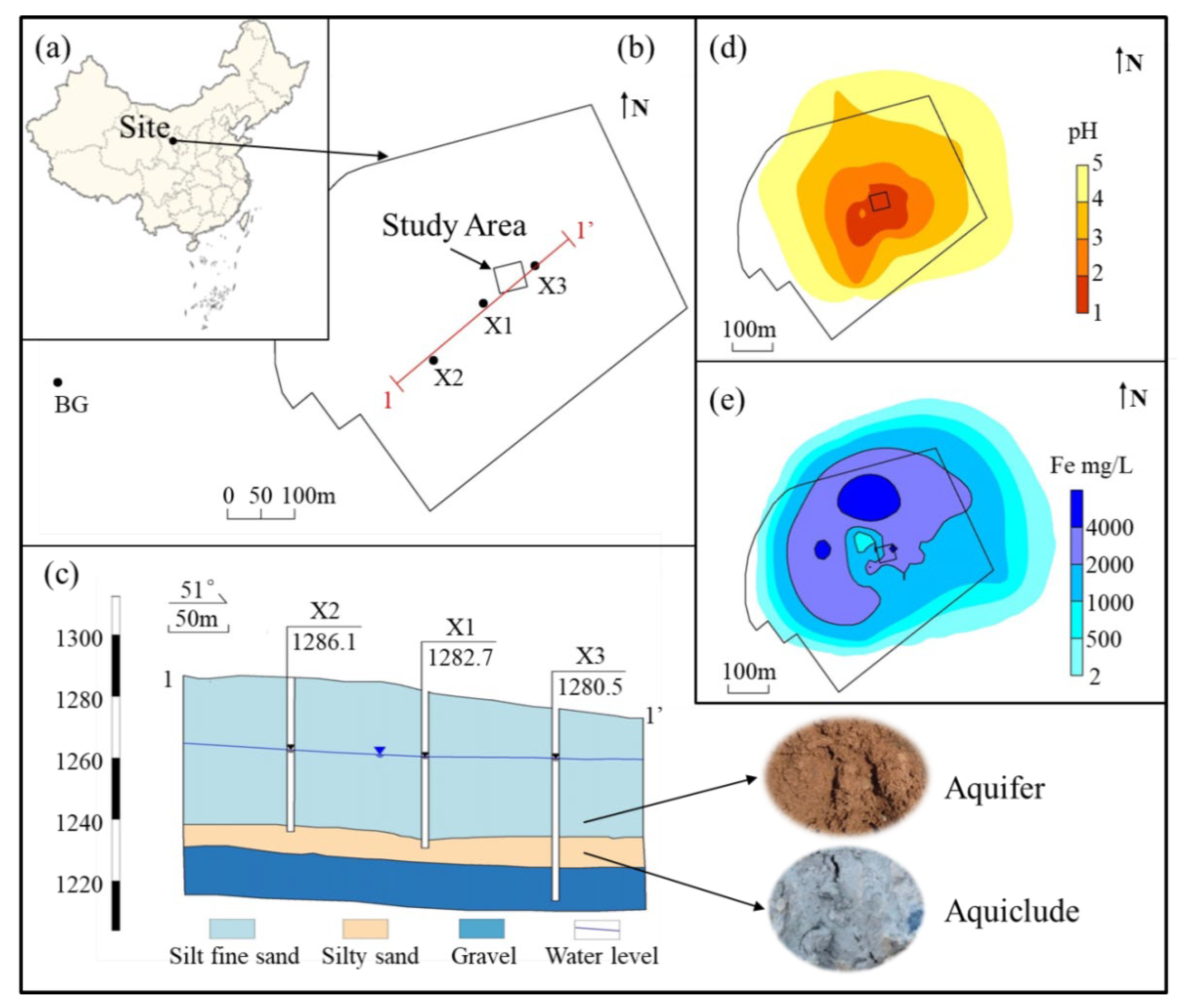
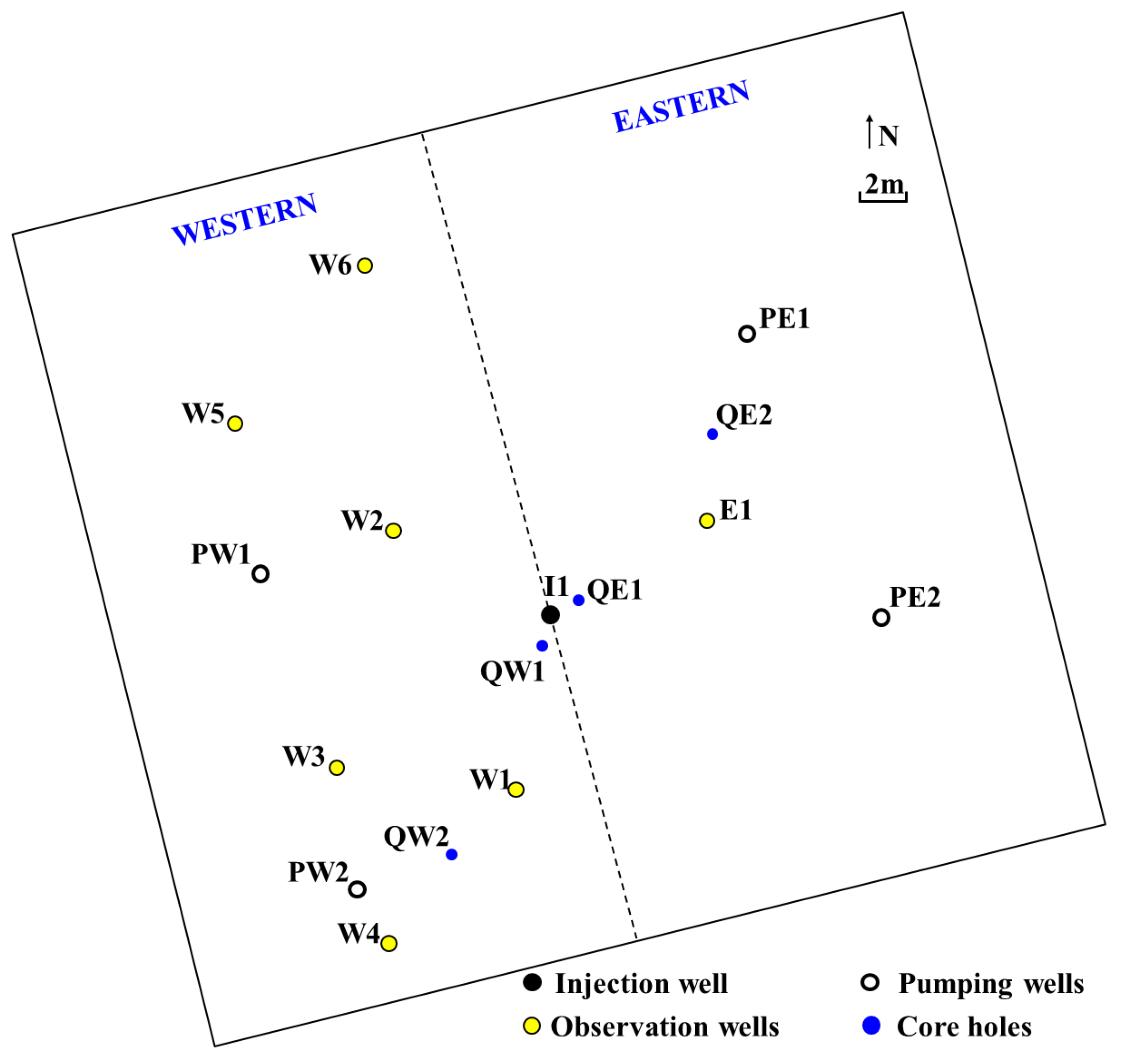
2.1. Study Site

The study site is located in the desert area of China. A factory there produced dye intermediates from 1998 to 2014. Groundwater pollution was caused by the discharge of wastewater to the outside of the factory. Sulfuric acid was one of the main raw materials. Therefore, the groundwater is strongly acidic, with a pH of 1~3.

2.1.1. Hydrogeology Conditions

The unconfined aquifer was mainly Quaternary silty-fine sand, and the water level was 13.9~19.7 m below the surface. The thickness was about 25 m with a permeability coefficient of about 3 m/d, while the porosity was about 0.2. The aquiclude was silty clay with a thickness of about 3 m. The minerals were dominated by clay minerals as well as calcite, dolomite, pyrite, etc., which easily react with acid and dissolve. The confined aquifer under the aquiclude was about 100 m thick with the interbedded pebble gravel and silty clay. The confined aquifer was a groundwater resource rich in amount and quality.

2.1.2. Characteristics of Groundwater Pollution

The polluted area of pH less than 3 was about 51,600 m² in the site. The study area is located in the heavily polluted groundwater area (Figure 1d) with strong acidity. Since the aqueous medium contained a large amount of iron-bearing minerals that can be easily dissolved by the acidic groundwater, this resulted in a high Fe concentration in the groundwater, up to 8900 mg/L.

According to the characteristics of groundwater acid pollution, the study area was set up in the area with the strongest acidity (pH < 3) (Figure 1b). The study area was about 1596 m², 42 m long and 38 m wide. It was divided into east and west, two areas by the injection well I1. The specific locations of injection wells, pumping wells and monitoring wells are shown in Figure 2. The pH of the observation wells W1~W6 on the western zone was 1.81~2.66, and the pH of the observation well E1 on the eastern zone was 1.2. The iron concentration in the western zone was 64.3~264.2 mg/L, and the concentration in the eastern zone was as high as 8880 mg/L. In order to control and remediate polluted groundwater, several pumping wells had been set up and extracted for 5 years on the site, but the increase in pH was extremely slow. According to the long-term monitoring well data of X3, the pH was still fluctuating between 0.4 and 1.4 (Figure S1). So, to solve the problem of acid groundwater corroding the aquiclude as soon as possible, a combination of pumping and injection to inject alkaline water was proposed in order to rapidly increase the pH and reducing environmental risks.

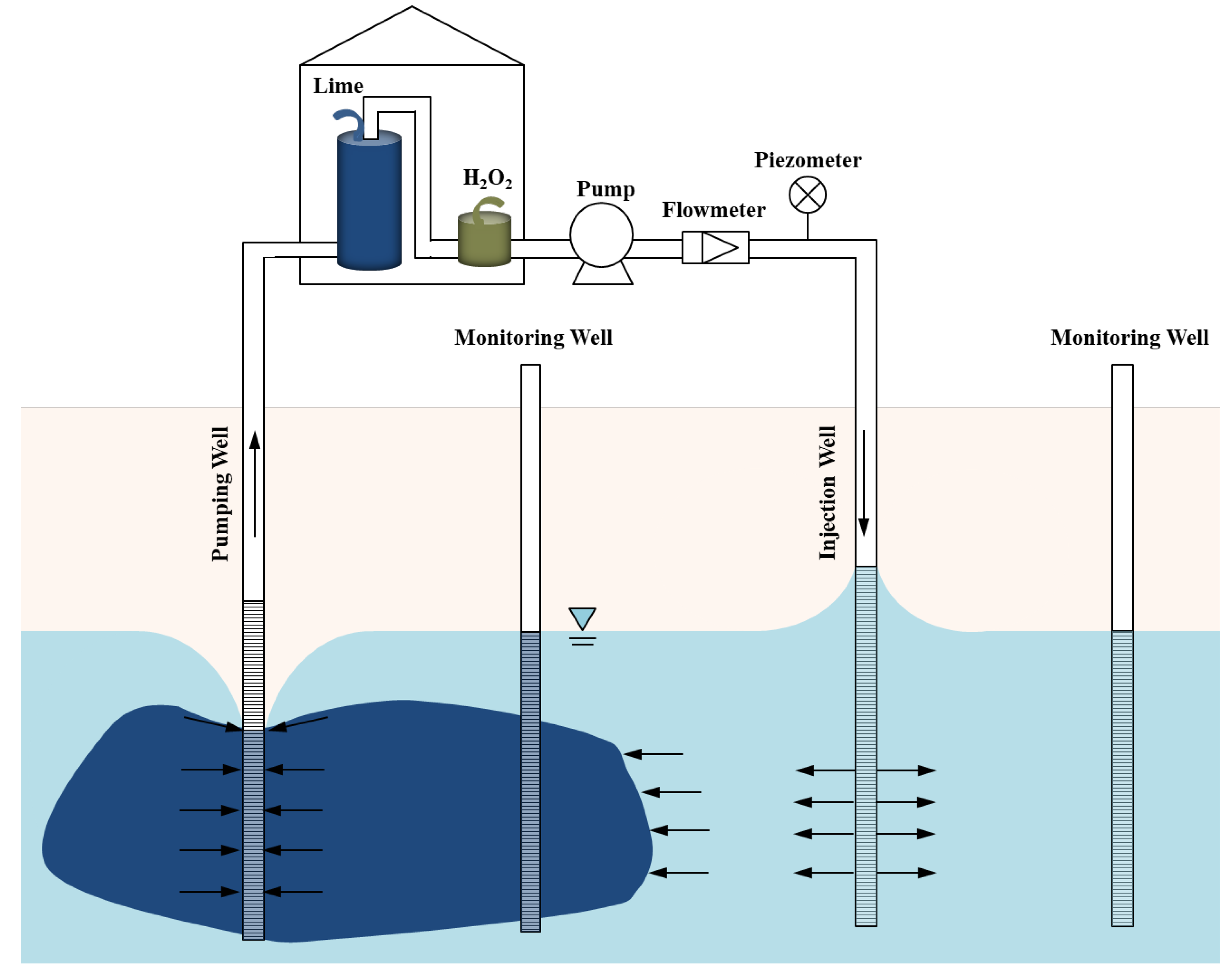
2.2. Operational Details

2.2.1. Pump–Treat–Inject Process

The pump–treat–inject process is shown in Figure 3. Firstly, the acid-polluted groundwater with pH < 2 was extracted from the pumping well, and the Fe concentration was 912~2180 mg/L, then transported to the surface treatment system (

Table 1. Water quality of monitor wells, pumping and injecting water in the study area.

Index	Pumped Groundwater	Injection Water (Average Value)	Monitor Well
			Western Zone						Eastern Zone
			W1	W2	W3	W4	W5	W6	E1
pH	1.29~1.8	8.5	2.15	2.24	2.03	1.81	2.57	2.66	1.2
Fe (mg/L)	912~2180	—	213.6	229.1	264.2	243.1	66.02	64.3	8880
COD (mg/L)	1249~4650	1610	820	94.5	1226.5	2287	320.5	311	9240
HAc (mg/L)	1050~3900	1560	728	520	1086	2130	290	280	8224
Distance to the injection well (m)			8	8.2	12.3	16.6	17.15	18.2	8.45

).

After adjusting the pH with lime milk, the pH of the effluent was stabilized at about 8.5, and the Fe formed precipitation as the pH was raised to alkaline, so the Fe concentration was lower than the detection limit. The precipitation in the treated groundwater was removed by pressure filtration. Finally, the treated groundwater was injected back into the aquifer from the injection well.

In addition, there was also chemical oxygen demand (COD) pollution in the groundwater. The COD concentration in the extracted groundwater was 1249~4650 mg/L. During the treatment at the ground station, part of the organic matter was oxidized and removed by hydrogen peroxide, and the COD was reduced to about 1610 mg/L. The main component was acetic acid, which was difficult to oxidize by hydrogen peroxide. So, the main goal of this study was to increase the pH of groundwater so as to reduce the risk of acid groundwater corroding the aquiclude and avoid contaminating the underlying confined aquifer. Since acetic acid is less biologically toxic and can be used as a good carbon source by microorganisms and be gradually removed from the aquifer by natural attenuation, it will, therefore, not be discussed in depth in this study.

2.2.2. Experimental Process

The study area was divided into the eastern zone and the western zone by the center injection well (I1) (Figure 2), and there were two pumping wells, PW1 and PW2 and PE1 and PE2 at the two zones, respectively. (The distance to the water injection wells was 15 m, 13.3 m, 15.7 m and 15.1 m, respectively.) The open and close of the pumping wells on both sides can control the flow direction of the injected water. The pumping wells in the western zone (PW1 and PW2) were opened during the whole process, and the pumping wells in the eastern zone (PE1 and PE2) were opened on the 26th day. Therefore, most of the injected water flowed to the west in the previous stage. Combined with the injection pressure, the experiment was divided into 2 major stages (

Table 2. Water injection pressure, volume and pumping wells at each stage.

Stage	Stage 1			Stage 2	Total
	Stage 1.1	Stage 1.2	Stage 1.3
Time	0~8th	9~19th	20th~30th	31st~57th	57 d
Injection pressure (MPa)	0~0.2	0.24~0.25	0.28~0.29	0.3~0.32	—
Injection volume (m3)	2022	2783	2671	8186	15,662
Pumping wells	PW1, PW2			PW1, PW2, PE1, PE2	—

). The injection test lasted for 57 days and the total amount of water injected was 15,662 m³. The pumping rate of PW1 and PW2 was about 3 m³/h, of PE1 and PE2 was about 6 m³/h and the total pumping volume was about 17,424 m³.

At the first stage (the first 30 days), in order to determine the relationship between the water injection pressure and the displacement efficiency, the step-by-step pressurization method was adopted for water injection, and the pressure was increased from 0 to 0.29 MPa in three steps. In order to study the change in injection rate and the effect on pH, as well as the change in the permeability of the 6 observation wells W1~6, which were set up at different distances (8 m, 8.2 m, 12.3 m, 16.6 m, 17.15 m, 18.2 m to the water injection wells, respectively) under different pressures.

The second stage was from the 31st to the 57th day, with a given pressure of 0.3 to 0.32 MPa. The aim of this stage was mainly to observe the operation of the eastern zone at a higher constant pressure. There was an observation well, E1 (8.45 m away from the water injection well), in the eastern zone. The displacement efficiency of the 1.1 stage of the western area was compared, that is, the attenuation of the injected water volume and the amount of precipitation.

2.3. Sample Collection and Analysis

2.3.1. Water Sample Analysis

During the test period, water samples from each monitoring well were taken regularly with Baylor tubes and then passed through a 0.25-micrometer filter membrane before testing. PH was measured on-site with a multiparameter water quality monitor (Manta, Eureka). COD was determined by a COD rapid analyzer (5B-3C, Beijing Lianhua Yongxing Technology Development Co., Ltd, Beijing, China). Fe was measured by inductively coupled plasma emission spectroscopy (iCAP 7000, Thermo, Waltham, MA, USA) at a wavelength of 259.94 nm.

2.3.2. Core Analysis

In order to verify the occurrence of precipitation and compare the amount of precipitation of the different distance to the injection well at different zones, two coring holes were set up in the two zones, respectively (Figure 2), after the experiment. QW1 and QE1 were 1 m away from the injection well and QW2 and QE2 were 11.5 m away. A control point (OS) at the pH≈2 area outside the experimental area and a background point (BG) were set. About 1 m of core was taken at the upper, middle and lower depths of the aquifer at each point, respectively, and mixed evenly. Then, 1 mol/L HCl was used to extract the iron precipitate on the core surface referring to the BCR leaching method for heavy metal acid soluble state [40]. Since 1 mol/L HCl cannot completely dissolve all iron minerals on the aqueous medium in a short period of time, this part of the dissolution can be considered as the less stable secondary iron-bearing minerals that were used to characterize the precipitation amount on the aqueous medium surface during the experiment. A total of 20 mL of 1 mol/L HCl and 10 g of core in 40 mL were put in a brown reagent bottle, and then, we placed the bottle on a 25 °C shaker and shook it for 16 h at 200 rmp. After sampling, it was passed through a 0.25-micrometer filter membrane to measure Fe. The test method is the same as that described in 2.3.1. The core surface topography was analyzed by cold field emission scanning electron microscopy (S-4800, Hitachi, Japan).

2.4. Analysis of the Data

2.4.1. Breakthrough Time

The migration process from injection wells to pumping wells and monitoring wells is a typical convective diffusion process. The solute concentration in observation wells and pumping wells showed an s-shaped upward trend [41]. The time from the start of injection to the solute concentration increase (or decrease) to 50% of the stable value is defined as the injected water migration to the monitoring well, which is recorded as t_a. The midpoint of the concentration of the breakthrough curve is only determined by the convection process and is not affected by the dispersion effect, so the particle convection process is identified by obtaining the time corresponding to this midpoint [42]. A representative S-type curve Boltzmann function is chosen for C–t series fitting to calculate the time t_a [42,43].

$$C=\frac{C_{1 }{- C}_2}{1+exp\left(\frac{{t - t}_a}{d_t}\right)}{+C}_2$$

(1)

C₁ is the initial concentration before injection (mg/L), C₂ is the concentration in the observation well after injection increase/decrease to a stable value (mg/L), t_a is the center of the curve (d) and d_t is the time constant.

2.4.2. Neutralized H⁺ Content

During the injection, H⁺ in the groundwater was consumed by neutralization with injected water. This amount of H⁺ can be calculated according to the OH⁻ concentration of injected water and the difference in OH⁻ concentration when it reached the observation well. The time difference between the breakthrough time of COD and pH in the observation well was the time used for neutralization that can be calculated by the following formula:

$$t_{ne}{=t}_{pH} {- t}_{COD}$$

(2)

$$\mu =\frac{S}{t_{COD}}$$

(3)

$$q_n=\mu t_{ne}{LMn(C}_I {- C}_a)$$

(4)

$T_{ne}$, $t_{COD}$, and $t_{pH}$ are neutralized time, breakthrough time of COD and pH in the observation well (d), μ is actual velocity of groundwater (m/d), $q_n$ is the amount of neutralized H⁺ (mol), S is the distance between observation well and injection well (m), L is the length of the water-passing section at the observation well in the equilibrium area (m) (using the numerical simulation method to construct a numerical model and based on the particle tracking module, acquire the streamline of each equilibrium zone, thereby the length of the water-passing section is obtained), M is the thickness of aquifer thickness (the site aquifer thickness is 25 m), n is porosity (0.2) and $C_I$ and $C_a$ are the OH⁻ concentration of the injected water and the OH⁻ concentration of the observation well breakthrough, respectively (mol/L).

2.4.3. Extracted H⁺ Content

The amount of extracted H⁺ is calculated by the equilibrium method. The area surrounded by the streamline from each pumping well to the injection well obtained by the numerical model is an equilibrium area. The time for the injected water breakthrough to the pumping well is an equilibrium period. The amount of H⁺ extracted in each equilibrium zone can be calculated according to the volume of water pumped and the H⁺ concentration of the extracted water using the following formula:

$$Q_P{=Q}_{OS}{+Q}_{IN}$$

(5)

$$Q_p{C}_P{=Q}_{OS}{C}_{OS}{ +Q}_{IN}{C}_{IN}$$

(6)

The proportion of the injected water in the equilibrium area of the pumped water:

$$x=\frac{Q_{IN}}{Q_P}=\frac{C_{OS }{- C}_p}{C_{OS}{ - C}_{IN}}$$

(7)

The amount of extracted H⁺ is:

$$x=\frac{Q_{NN }}{Q_P} \frac{C_{OS}{ - C}_p}{C_{OS}{ - C}_{IN}}$$

(8)

$Q_P$ is the pumping volume of the pumping wells in the equilibrium zone (L); $Q_{OS}$ and $Q_{IN}$ are the volume of water entering the pumping well from outside and inside the equilibrium zone, respectively, (L), $C_P$, $C_{OS}$ and $C_{IN}$ are the H⁺ concentration of the pumping well, outside the equilibrium zone and inside the equilibrium zone, respectively, (mol/L), and $q_P$ is the amount of extracted H⁺ (mol).

3. Results and Discussion

3.1. Displacement of Acidic Groundwater by Injected Water

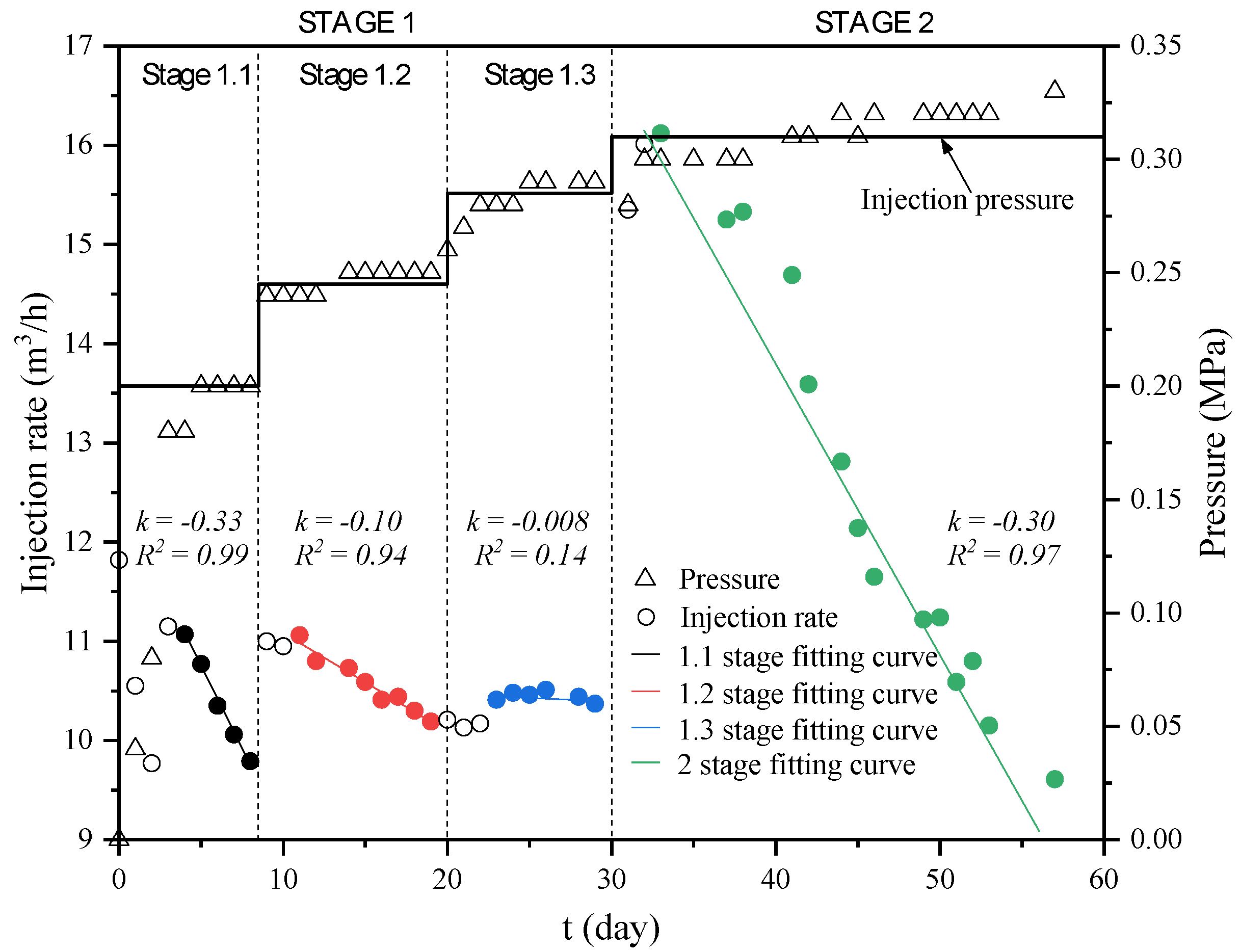
3.1.1. Water Injection Process

In stage 1 (the first 30 days), in order to study the relationship between the water injection pressure and displacement efficiency, the injection was carried out in a step-by-step pressurization method (Figure 4), and the pressure was increased from 0 to 0.29 MPa in three steps. The pumping wells PW1 and PW2 on the western zone were opened, and PE1 and PE2 on the eastern zone were closed, so most of the injected water flowed to the west side. The pressure in stages 1.1 to 1.3 gradually increased and the initial injection rates were 11.82 m³/h, 11 m³/h and 10.3 m³/h, respectively. The injection rate in the first two stages gradually decreased with time and was basically stable in the 1.3 stage. The injection rate (q) and time (t) were fitted with linear equation and the slope was the decay rate of each stage (Text S1). The decay rates of the three stages were 0.33, 0.1 and 0.008, respectively, indicating that with the increase in pressure and the injected water flow to the periphery, the decay rate decreased. In stage 2 (31~57 days), the injection pressure was high and stable. Due to the opening of the eastern zone’s pumping wells and the high injection pressure, the injected water mainly flowed to the east side and the initial injection rate increased to 15.53 m³/h, which was significantly higher than that in the 1.1 stage. However, as the injection progressed, the injection rate also decreased linearly with a decay rate of 0.30, slightly less than the 1.1 stage. Stage 1 injected 7476 m³ of water in 30 days and stage 2 injected 8186 m³ of water in 27 days. Although the decay rate gradually decreased with the gradual pressurization, the decay rate of stage 2 was similar to that of stage 1.1, but due to the large initial flow rate, the total injection volume was still higher than that of stage 1, and the per unit time water injection efficiency was improved by more than 20%.

The decrease in the initial injection rate and the injection volume at each stage may be caused by the decrease in permeability of the aquifer. The groundwater was acidic with a pH of less than 3, while the injected water was alkaline with a pH of about 8.5, which led to the increase in pH in the groundwater. Due to the high iron concentration in groundwater, precipitation was easy to generate when pH rose and the precipitation deposited in the pores of the aquifer, causing blockage and poor permeability. However, as the injected water flowed to the periphery and the injection pressure increased, the water-passing section became wider and the groundwater flow rate was faster. The faster flow rate shortened the residence time and reduced the amount of precipitation. At the same time, the cross-section of water increased, less precipitation was distributed to each pore and the injection rate decay was gradually reduced. The initial injection rate of stage 2 was high mainly because most of the water flowed to the east side where the degree of blockage was low and the groundwater flow rate was faster when the pressure was high, so the neutralization time was shortened, resulting in the precipitation being slightly less than in the 1.1 stage. As the injected water’s pH increased, the precipitation gradually formed and the injection rate decreased.

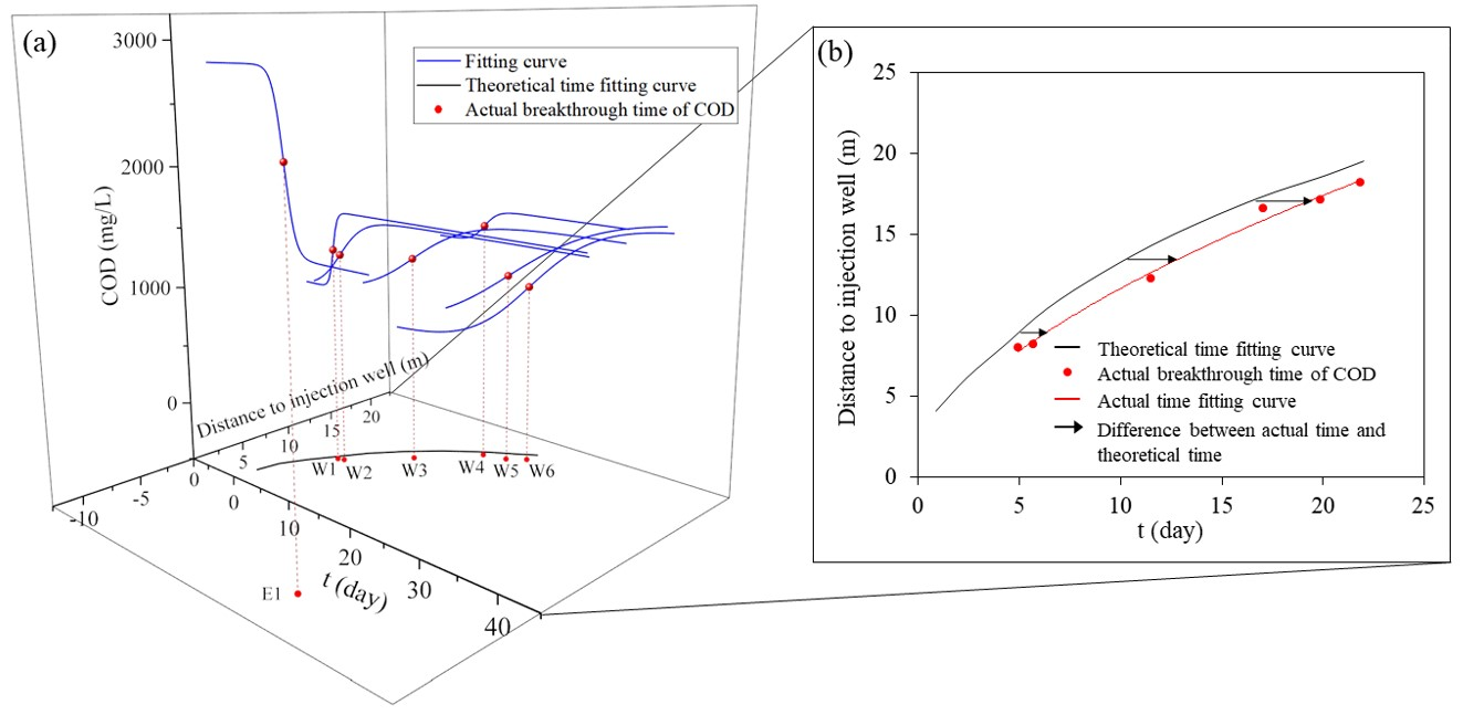
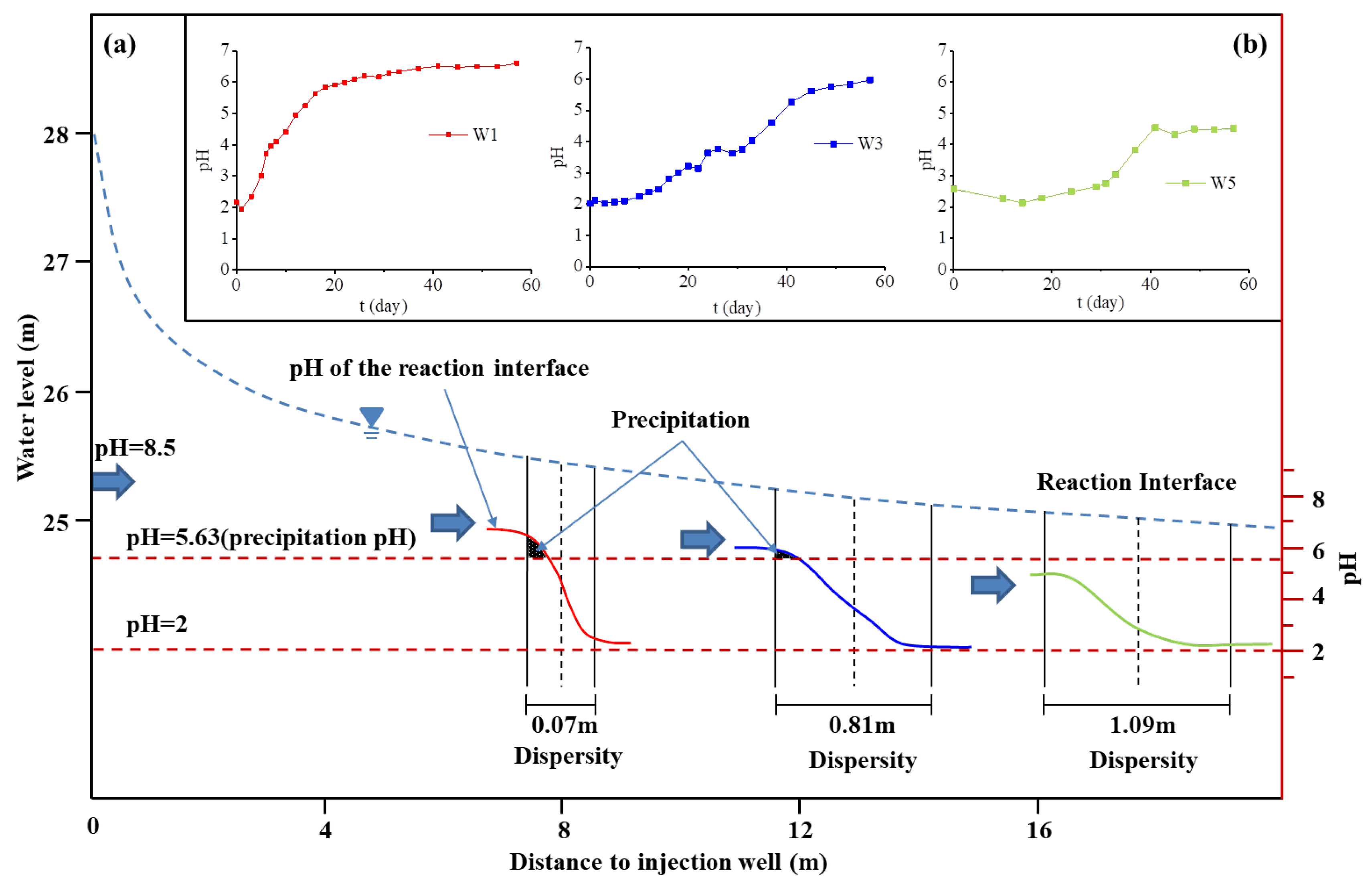
3.1.2. Flow and Dispersion Process of Acidic Groundwater

The displacement process of injected water to groundwater can be characterized by the change in the COD concentration of observation wells at different distances. This was mainly due to the large difference in COD concentrations between injected water and groundwater. Additionally, the pollutants, such as acetic acid represented by COD, mainly flow and disperse. In the process of groundwater displacement, pollutants, such as acetic acid represented by COD, were mainly migrating by convection and dispersion. Therefore, the migration of injected water and polluted acidic groundwater can be reflected by observing the change in COD concentration with time at the monitoring well.

With the progress of water injection, the COD concentration of the observation well on the western zone gradually increased (Figure 5), and the COD concentration of the observation well on the eastern zone quickly decreased to the injected water concentration after the pumping well on the eastern zone was opened (26 d). The COD concentration–time series was fitted with the Boltzmann function, and the midpoint of the concentration was the breakthrough time (t_COD) of the injected water (Table S1, Figure S1), which can reflect the flow process. The injected water migrated to W1 and W2 on the 5~6th day, to W3, W4 and W5 on the 11~20th day, and to W6 and E1 on the 21.82nd to the 26.5th day, respectively. Fitting of the actual breakthrough time (t_COD) and migration distance of injected water was conducted and then compared with the theoretical migration curve. (See Table S2 for details.) The numerical simulation method was used to build a numerical model (Text S2). The water level data were extracted from the model and divided to acquire the hydraulic gradient of each subdivided unit. The migration velocity and migration time of each unit were calculated according to the permeability coefficient and the pumping test before the experiment. The theoretical migration curve was obtained by fitting the time and migration distance according to the unchanged permeability coefficient and did not take precipitation into account. The fitting curve of actual breakthrough time is on the right side of the theoretical migration curve, indicating that the actual breakthrough time lags behind the theoretical value and the farther the distance is, the longer the lag time is (Figure 5b). The actual migration time was used to calculate the migration velocity (Table S3), and the velocities of the two observation wells at different distances in the same radial direction were compared. The speed of migration from injection well I1 to W1 was 1.62 m/d, from W1 to W4 was 0.71 m/d, from I1 to W2 was 1.44 m/d and from W2 to W5 was 0.63 m/d. This demonstrated that the farther the injected water diffused, the lower the hydraulic gradient, and the longer the distance, the slower the migration speed. With the progress of injection, the rate of COD concentration increased/decreased, and injected water concentration in each observation well was also different. It rose faster to the stable concentration at closer observation wells due to the dispersion effect, and the farther the distance, the longer the dispersion. When injected water migrated to W1 and W2, the dispersion was only 6~7 cm, while it migrated to 16~17 m when the dispersion was about 1.5 m. In addition, the increase in pressure can also slow down the dispersion effect, so the COD concentration of E1 decreased from breakthrough to stable faster than W1 and W2.

3.1.3. Attenuation of Permeability of Aqueous Medium

According to the numerical simulation results, water level data were extracted. W1~W4 and W2~W5 were two sets of observation wells in the same radial direction, respectively. According to the actual velocity and water level data, the permeability coefficients of I1~W1 and W1~W4 were 1.4 m/d and 2.59 m/d, respectively, and the permeability coefficients of I1~W2 and W2~W5 were 1.33 m/d and 2.48 m/d, respectively (Table S3). It follows that the permeability coefficient near the water injection well reduced significantly, while the permeability of the farther area decreased less, indicating that the blockage was mainly generated in the area close to the injection well.

3.2. Displacement–Neutralization Process of Acidic Groundwater

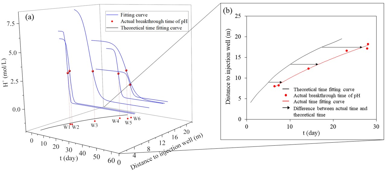
3.2.1. Dynamic Variation of Groundwater pH

In order to observe the displacement–neutralization process of acidic groundwater, the observation of pH in the observation wells was carried out, and the results are shown in Figure 6. The change characteristics of pH were similar to COD in general. The closer the distance was, the earlier the breakthrough time was and the faster it was to stabilize. The pH of monitoring wells all gradually increased to more than 4.5 (Figure 9). The H⁺ of the W1 that was close to the injection well was 4.57 mol/L on the 6th day and rapidly decreased to about 0.1 mol/L on the 10th day, and the final pH was about 6.5 (Figure S2). On the other hand, the H⁺ of the farther observation well W5 was 2.29 mol/L on the 29th day and decreased to 0.15 M in 37 days with a final pH of around 4.5.

The pH did not rise to the same level as the injected water because of the neutralization of the medium that consumed OH⁻ during the migration of the injected water. The farther the migration, the more OH⁻ was consumed, so the pH of the farther observation wells increased less. As the injected water migrated, an acid–base water neutralization interface formed as a result of the dispersion with groundwater. The pH of the injection well side was high, while the pH of the groundwater side was low, and the pH gradually decreased from the injection water side to the groundwater side. The interface gradually migrated to the periphery with the injection process. The farther the migration, the longer the dispersion distance, and the larger the interface width, the slower the pH rise will be.

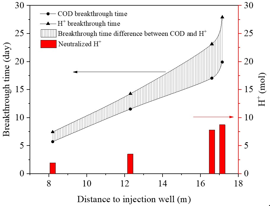
3.2.2. Neutralization Amount of H⁺ in Groundwater

Although the overall trend of pH was basically the same as that of COD in each monitoring well, the time pH rose obviously lagged behind that of COD (Figure 7). This may be because of the neutralization between the acidic groundwater and injected water consuming the H⁺ and OH⁻ at the acid–base water interface. The time difference was the neutralization time. A numerical simulation method was used to build a numerical model to calculate the amount of neutralized H⁺. Based on the particle tracking module, four equilibrium zones were determined, named PW1, PW2, PE1 and PE2, respectively (Text S2). According to the envelope of each equilibrium area, the length of the water-passing section of each observation well can be obtained. Combined with the groundwater flow rate, the H⁺ neutralization amount can be calculated (Table S4).

As the injected water moved outward, the farther the observation wells in the west area were, the longer the neutralization time was, and the amount of neutralized H⁺ gradually increased (Figure 7). From W1 to W5, the amount of H⁺ neutralization increased from 1.95 mol to 8.72 mol. The neutralization time of E1 in the eastern zone was slightly shorter than the observation wells W1 and W2 of the approximate distance in the western zone, indicating that the increase in pressure was beneficial to shorten the neutralization time and reduce the amount of H⁺ neutralized. The neutralized H⁺ amounts of PE1 and PE2 in the eastern zone were 1.67 mol and 5.23 mol, respectively, and PW1 and PW2 in the western zone were 8.72 mol and 7.81 mol, respectively. From this, it can be speculated that the neutralization amount and precipitation amount in the eastern zone were less than the western zone.

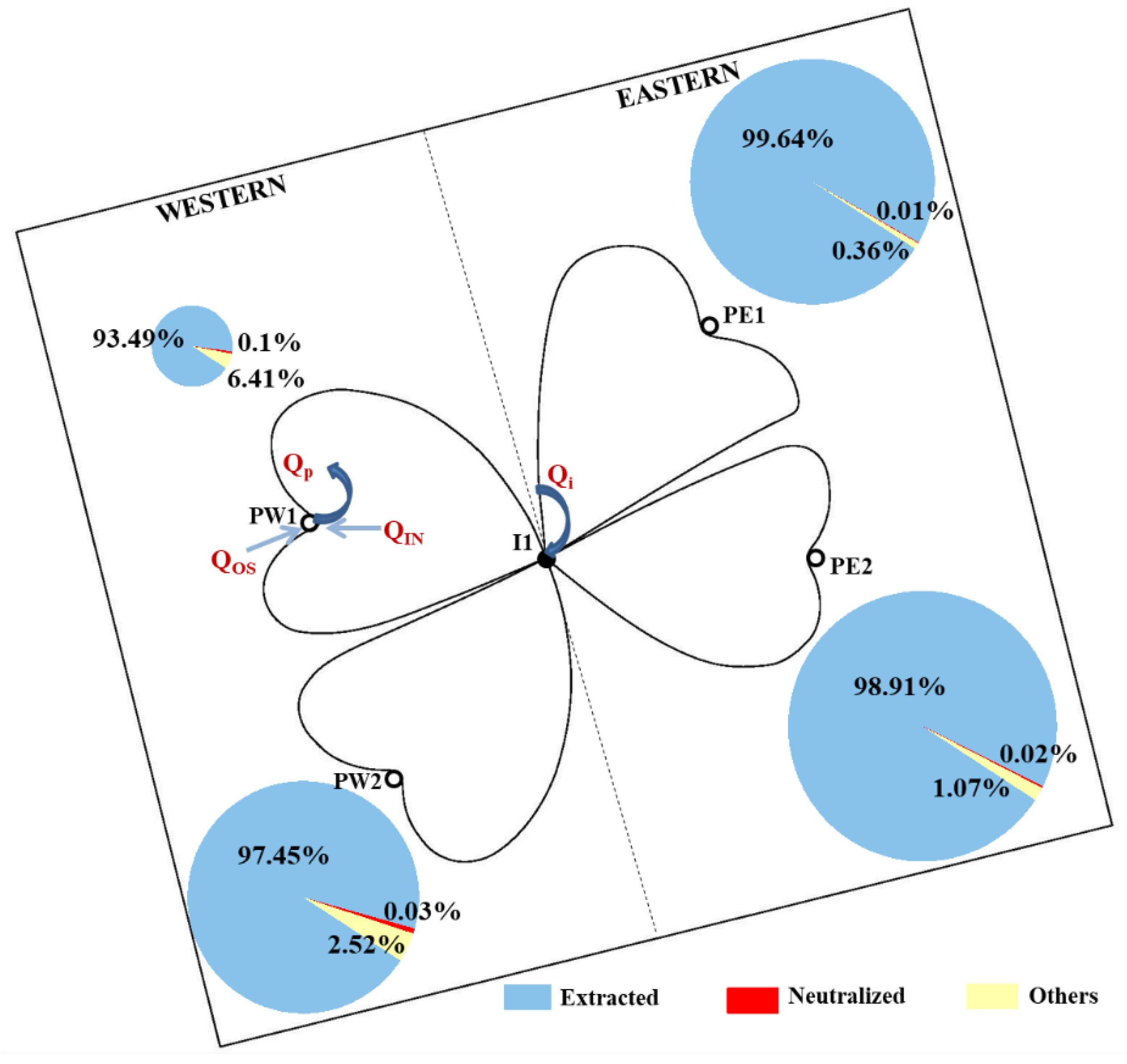
3.2.3. Equilibrium Analysis of H⁺ in Groundwater

On the basis of the H⁺ neutralization amount analysis, the displacement amount of H⁺ in groundwater will be further counted and the equilibrium analysis of H⁺ in groundwater will be carried out. The four equilibrium zones are shown in Figure 8. The equilibrium period was calculated as the injected water migrated to the pumping well; that is, the groundwater in the equilibrium zone was completely displaced once. The balance item of each zone mainly includes the groundwater volume extracted from the equilibrium zone, outside the zone and the total pumped water. The calculation method and process of each equilibrium item are shown in the Supplementary Materials.

After the start of the injection experiment, the pH of the pumping wells also gradually increased. Before that, according to the long-term monitoring data of the pumping well in the heavily polluted area, the pH remained basically stable for a long time (Figure S3), and the pH was as low as about 1. Since the pH of the study area was slightly higher than that of the outside after the start of water injection, the proportion of the water extracted in the study area increased, so the pH of the pumping wells increased. When the injected water had completely displaced the groundwater of the equilibrium zone, the pumping wells extracted the low-pH groundwater outside the study area and the injected water at a stable ratio, and then the pH rose to a stable level. Taking the initial pH of the pumping well as the pH of the outside and the pH in the stable state as the pH in the equilibrium zone, the H⁺ amounts extracted from the equilibrium areas of PW1, PW2, PE1 and PE2 were 8085.62 mol, 25,049.46 mol, 27,048.87 mol and 29,433.67 mol, respectively (

Table 3. Neutralized, extracted and other part amounts and proportion of H⁺ in each equilibrium area.

Equilibrium Area	Total (mol)	Neutralized		Extracted		Others
		Amount	Proportion (%)	Amount	Proportion (%)	Amount	Proportion (%)
PW1	8648.69	8.72	0.10	8085.62	93.49	554.34	6.41
PW2	25,705.49	7.81	0.03	25,049.46	97.45	648.22	2.52
PE1	27,146.96	1.67	0.01	27,048.87	99.64	96.42	0.36
PE2	29,756.84	5.23	0.02	29,433.67	98.91	317.95	1.07

).

According to the envelope area and interpolation calculation results of each equilibrium zone, the total amount of H⁺ in each zone was 8648.69 mol, 25,705.49 mol, 27,146.96 mol and 29,756.84 mol, respectively. The extracted amount from each equilibrium zone accounts for more than 93% of the total. Neutralization accounted for less than 0.2%. The rest is due to calculation errors and other parts, such as residuals on the medium, accounting for 0.3~7%. It can be seen that the pH increase in each zone was mainly due to the displacement of injected water.

Although the proportion of neutralization was small, it was the neutralization that obviously led to the reduction in permeability, thereby reducing the efficiency of injection–extraction, which had become an important restrictive factor for the restoration project and cannot be ignored. It is necessary to develop the mechanism analysis and optimized design of adsorption engineering process parameters for the blocking problem.

Above all, the main principle of the pumping–injection process is the displacement process, which plays a major role in the remediation process. In addition, the neutralization of the acid–base water contact will also increase the pH, which is the secondary contribution. Therefore, the remediation mechanism of this site is the displacement–neutralization mechanism.

3.3. Blocking Mechanism

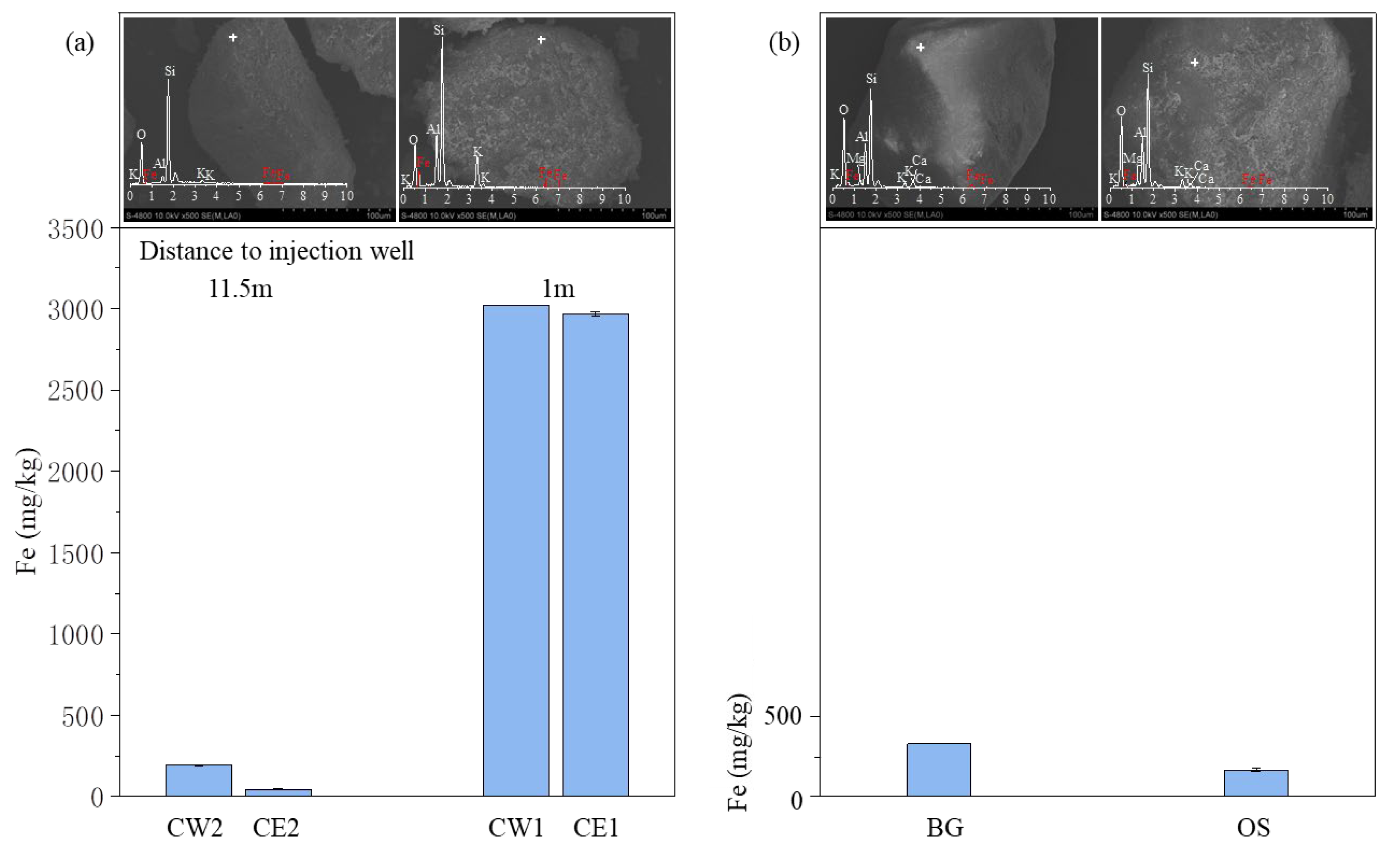
3.3.1. Iron Concentration

The iron concentration of each monitoring well gradually decreased due to the displacement of the injected water. The iron of observation wells W1~3, which were closer to the water injection well, were lower than the detection limit when the pH rose to about 5.63 (Figure 9), indicating that under the hydrochemical conditions of this site, iron began to precipitate at this pH. Then, the slow pH rise may be caused by the precipitation of iron hydrolysis and the supply of H⁺ [11]. When the pH of W4 was 3.22, the iron decreased to 0.286 mg/L and the pH was always lower than 5.63, which did not meet the conditions for precipitation, and the iron concentration finally dropped to undetectable levels because the injected water completely displaced the groundwater. However, the pH of W5~6 did not reach 5.63, iron was still detected in a certain amount after the injected water was displaced completely and the concentration was relatively stable, which may be due to the continuous desorption of iron adsorbed on the medium.

$${Fe}^{3+}{+H}_{2}O\to { FeOH}^{2+}{+H}^{+}$$

(9)

$${Fe}^{3+}{+2H}_{2}O\to { FeOH}_2^{+}{+2H}^{+}$$

(10)

$${Fe}^{3+}{+3H}_{2}O\to { Fe\left(OH\right)}_{3\left(s\right)}{+3H}^{+}$$

(11)

$${Fe}^{3+}{+2H}_{2}O\to { Fe\left(OOH\right)+3H}^{+}$$

(12)

According to the change in iron concentration combined with the law of pH increase, it can be seen that 5.63 is the critical pH at which precipitation occurs. The closer to the injection well the narrower neutralization interface (Table S5) was, the faster the pH increased (Figure 10) and soon rose to above 5.63, while the iron concentration was still high enough to produce precipitation. Therefore, the closer to the injection well, the greater the amount of precipitation was. Whereas, in the area far from the injection well, pH could not rise to the critical pH of 5.63 due to the neutralization of the medium along the process, and as the neutralization interface is wide, the pH rose slowly. When the pH was still low, the iron concentration dropped to a very low concentration owing to the displacement of injected water and the conditions for precipitation were not met. With the increased injection pressure, the precipitation interface gradually expanded. In stage 1.1, the injection rate reduced linearly, indicating that the precipitation had been formed. After pressurization in stage 1.2, the velocity of groundwater increased and promoted the outward migration of injected water simultaneously, the precipitation interface around the injection well expanded outward and continued to generate precipitation and the injection rate decreased again. However, in stage 1.3, it continued to increase the pressure and the injection rate was basically stable. This was because the injected water diffused farther and the pH could not rise to 5.63, while the iron had dropped to a very low concentration that could not produce precipitation. So, the permeability of the aquifer did not change, and the flow rate was basically stable. In stage 2, the pressure increased and most of the water migrated to the east. Due to the formation of precipitation, the injection rate also dropped linearly, and the decay rate was slightly lower than that in stage 1.1, indicating that the pressure increase can slightly reduce the production of precipitation.

3.3.2. Mineralogical Analysis

After the test, cores were taken from the eastern zone, western zone, the control point OS (areas with pH ≈ 2 outside the study area) and the background point BG. HCl was used to dissolve the iron precipitation on the core surface, and we compared the amount of iron precipitation in the area close to the injection well (1 m) and the area far away (11.5 m) of the two zones.

Fe dissolved in the two points CW1 and CE1 near the injection well in the study area was about 3000 mg/kg, which was significantly higher than the 162.8 mg/kg of OS (Figure 11). The Fe content of CW1 in the western zone was slightly higher than that of CE1 in the eastern zone. The Fe content of CW2 and CE2 at the two points far from the injection well were similar to that of OS and less than BG. Due to the difference in the content of iron-bearing minerals and dissolution on the surface of the medium, it can be seen that the iron precipitation at these two points was either very small or no precipitation was generated. Combined with the previous judgment, a small amount of precipitation occurred in the western zone far from the injection well. In summary, aquifer medium near the water injection well was covered by a large amount of iron precipitation, so a large amount of Fe was dissolved by HCl, while the amount of precipitation far away was very small. The precipitation in the east area was slightly less than that in the west, indicating that high injection pressure can reduce the formation of precipitation.

Comparing the surface topography of the two points CW1 and CW2 in the western zone, the outside point OS and the background point BG indicated that compared with BG under natural conditions, the surface of the medium became significantly uneven in the acidic environment. Additionally, some floccule obviously attached to the surface of the medium in the study area, while there were more on the surface of the point close to the injection well, which also showed that there is more precipitation closer to the well.

4. Conclusions

This paper was based on an acidic–high-iron-polluted site. Through a partition and staged water injection pressure experiment, we injected water with a pH of about 8.5 in a heavily polluted area with a groundwater pH of 1~3, and groundwater was pumped around to explore the remediation effect and influencing factors. The results showed that in the case of step-by-step pressurized water injection, the permeability was reduced due to the formation of precipitation, and the initial injection rate, injection volume and decay rate at each stage were decreased. The increase in pressure can slightly reduce the generation of precipitates. When the pressure increased from 0.2 MPa to 0.3 MPa, the water injection efficiency per unit time was increased by more than 20%. The principle of pump–injection remediation of acidic groundwater was mainly displacement, accounting for more than 93%, while neutralization only contributed less than 0.1%. Although the neutralization contribution was small, the neutralization interface was the main place for precipitation, which was the important constraint factor for the restoration project and cannot be ignored. The acid–base water neutralization interface was formed owing to the dispersion. The closer to the water injection well, the narrower the neutralization interface, the pH rising rapidly and the iron concentration being high result in more iron precipitation. In the area far from the injection well, pH did not rise to the condition to generate precipitation due to the neutralization of the medium along the process, and the iron concentration dropped to a very low concentration, so the conditions for precipitation were not met.

References

1. Güngör-Demirci, G.; Aksoy, A. Variation in time-to-compliance for pump-and-treat remediation of mass transfer-limited aquifers with hydraulic conductivity heterogeneity. Environ. Earth Sci. 2010, 63, 1277–1288. [Google Scholar] [CrossRef]
2. Ciampi, P.; Esposito, C.; Cassiani, G.; Deidda, G.P.; Rizzetto, P.; Papini, M.P. A field-scale remediation of residual light non-aqueous phase liquid (LNAPL): Chemical enhancers for pump and treat. Environ. Sci. Pollut. Res. 2021, 28, 35286–35296. [Google Scholar] [CrossRef] [PubMed]
3. Antelmi, M.; Renoldi, F.; Alberti, L. Analytical and Numerical Methods for a Preliminary Assessment of the Remediation Time of Pump and Treat Systems. Water 2020, 12, 2850. [Google Scholar] [CrossRef]
4. Truex, M.; Johnson, C.; Macbeth, T.; Becker, D.; Lynch, K.; Giaudrone, D.; Frantz, A.; Lee, H. Performance Assessment of Pump-and-Treat Systems. Groundw. Monit. Rem. 2017, 37, 28–44. [Google Scholar] [CrossRef]
5. Park, Y.-C. Cost-effective optimal design of a pump-and-treat system for remediating groundwater contaminant at an industrial complex. Geosci. J. 2016, 20, 891–901. [Google Scholar] [CrossRef]
6. Matott, L.S.; Rabideau, A.J.; Craig, J.R. Pump-and-treat optimization using analytic element method flow models. Adv. Water Resour. 2006, 29, 760–775. [Google Scholar] [CrossRef]
7. Thornton, S.F.; Baker, K.M.; Bottrell, S.H.; Rolfe, S.A.; McNamee, P.; Forrest, F.; Duffield, P.; Wilson, R.D.; Fairburn, A.W.; Cieslak, L.A. Enhancement of in situ biodegradation of organic compounds in groundwater by targeted pump and treat intervention. Appl. Geochem. 2014, 48, 28–40. [Google Scholar] [CrossRef]
8. Bortonea, I.; Ertob, A.; Nardoc, A.D.; Santonastasoc, G.F.; Chianesec, S.; Musmarrac, D. Pump-and-treat configurations with vertical and horizontal wells to remediate an aquifer contaminated by hexavalent chromium. J. Contam. Hydrol. 2020, 235, 103725. [Google Scholar] [CrossRef]
9. Kahler, D.M.; Kabala, Z.J. Acceleration of groundwater remediation by deep sweeps and vortex ejections induced by rapidly pulsed pumping. Water Resour. Res. 2016, 52, 3930–3940. [Google Scholar] [CrossRef]
10. Teramoto, E.H.; Pede, M.A.Z.; Chang, H.K. Impact of water table fluctuations on the seasonal effectiveness of the pump-and-treat remediation in wet–dry tropical regions. Environ. Earth Sci. 2020, 79, 435. [Google Scholar] [CrossRef]
11. Sadeghfam, S.; Hassanzadeh, Y.; Khatibi, R.; Nadiri, A.A.; Moazamnia, M. Groundwater Remediation through Pump-Treat-Inject Technology Using Optimum Control by Artificial Intelligence (OCAI). Water Resour. Manag. 2019, 33, 1123–1145. [Google Scholar] [CrossRef]
12. Takem, G.E.; Kuitcha, D.; Ako, A.A.; Mafany, G.T.; Takounjou-Fouepe, A.; Ndjama, J.; Ntchancho, R.; Ateba, B.H.; Chandrasekharam, D.; Ayonghe, S.N. Acidification of shallow groundwater in the unconfined sandy aquifer of the city of Douala, Cameroon, Western Africa: Implications for groundwater quality and use. Environ. Earth Sci. 2015, 74, 6831–6846. [Google Scholar] [CrossRef]
13. Vahedian, A.; Aghdaei, S.A.; Mahini, S. Acid Sulphate Soil Interaction with Groundwater: A Remediation Case Study in East Trinity. APCBEE Proc. 2014, 9, 274–279. [Google Scholar] [CrossRef]
14. Caraballo, M.A.; Macias, F.; Nieto, J.M.; Ayora, C. Long term fluctuations of groundwater mine pollution in a sulfide mining district with dry Mediterranean climate: Implications for water resources management and remediation. Sci. Total Environ. 2016, 539, 427–435. [Google Scholar] [CrossRef]
15. Shin, D.; Kim, Y.; Moon, H.S. Fate and toxicity of spilled chemicals in groundwater and soil environment I: Strong acids. Environ. Health Toxicol. 2018, 33, e2018019. [Google Scholar] [CrossRef]
16. Ha, Q.K.; Choi, S.; Phan, N.L.; Kim, K.; Phan, C.N.; Nguyen, V.K.; Ko, K.S. Occurrence of metal-rich acidic groundwaters around the Mekong Delta (Vietnam): A phenomenon linked to well installation. Sci. Total Environ. 2019, 654, 1100–1109. [Google Scholar] [CrossRef]
17. Appleyard, S.; Wong, S.; Willis-Jones, B.; Angeloni, J.; Watkins, R. Groundwater acidification caused by urban development in Perth, Western Australia: Source, distribution, and implications for management. Aust. J. Soil Res. 2005, 42, 579–585. [Google Scholar] [CrossRef]
18. Paulson, A.J.; Balistrieri, L. Modeling Removal of Cd, Cu, Pb, and Zn in Acidic Groundwater during Neutralization by Ambient Surface Waters and Groundwaters. Environ. Sci. Technol. 1999, 33, 3850–3856. [Google Scholar] [CrossRef]
19. Indraratna, B.; Pathirage, P.U.; Banasiak, L.J. Remediation of acidic groundwater by way of permeable reactive barrier. Environ. Geotech. 2017, 4, 284–298. [Google Scholar] [CrossRef]
20. Shin, D.; Lee, Y.; Park, J.; Moon, H.S.; Hyun, S.P. Soil microbial community responses to acid exposure and neutralization treatment. J. Environ. Manag. 2017, 204, 383–393. [Google Scholar] [CrossRef]
21. Sung, P.H.; Doyun, S.; Hee, S.M.; Young-Soo, H.; Seonjin, H.; Yoonho, L.; Eunhee, L.; Hyun, J.; Yu, S.H. A Multidisciplinary Assessment of the Impact of Spilled Acids on Geoecosystems: An Overview. Environ. Sci. Pollut. Res. 2020, 27, 9803–9817. [Google Scholar]
22. Jeon, I.; Nam, K. Change in the site density and surface acidity of clay minerals by acid or alkali spills and its effect on pH buffering capacity. Sci. Rep. 2019, 9, 9878. [Google Scholar] [CrossRef] [PubMed]
23. Zhang, Y.; Dai, Y.; Wang, Y.; Huang, X.; Pei, Q. Groundwater chemistry, quality and potential health risk appraisal of nitrate enriched groundwater in the Nanchong area, southwestern China. Sci. Total Environ. 2021, 784, 147186. [Google Scholar] [CrossRef]
24. Olías, M.; Cánovas, C.R.; Basallote, M.D.; Macías, F.; Pérez-López, R.; González, R.M.; Millán-Becerro, R.; Nieto, J.M. Causes and impacts of a mine water spill from an acidic pit lake (Iberian Pyrite Belt). Environ. Pollut. 2019, 250, 127–136. [Google Scholar] [CrossRef]
25. Zhang, Y.; He, Z.; Tian, H.; Huang, X.; Zhang, Z.; Liu, Y.; Xiao, Y.; Li, R. Hydrochemistry appraisal, quality assessment and health risk evaluation of shallow groundwater in the Mianyang area of Sichuan Basin, southwestern China. Environ. Earth Sci. 2021, 80, 576. [Google Scholar] [CrossRef]
26. Gazea, B.; Adam, K.; Kontopoulos, A. A review of passive systems for the treatment of acid mine drainage. Miner. Eng. 1996, 9, 23–42. [Google Scholar] [CrossRef]
27. Jiankang, Z.; Yong, Z.; Jin, C. Application Research on Pressure Recharge in Underground-water Source Heat Pump System. Explor. Eng. (Rock Soil Drill. Tunn.) 2010, 37, 55–58. [Google Scholar]
28. Wu, J.Q.; Zhang, J.Z.; Li, X.H.; Shi, F.F.; Zhang, P.; Bai, M. Experiment on artificial pressure re-injection of geothermal water in Xi’an suburb. J. Water Resour. Water Eng. 2014, 25, 215–218. [Google Scholar]
29. Zhao, B.l.; Mu, Z.Y.; Wu, J.X. Articifial Recharge of Groundwater (Translated Version); Water Conservancy Press: Beijing, China, 1980; pp. 32–33. [Google Scholar]
30. Du, X.Q.; Lu, Y.; Li, S.T.; Ye, X.Y.; Wang, Z.J. Mechanism, Prediction and Control of Suspended Matter Blocking in Artificial Recharge of Groundwater. In Proceedings of the 8th China Water Forum, Harbin City, China, 2–3 August 2010; p. 146. [Google Scholar]
31. Akhtar, M.S.; Nakashima, Y.; Nishigaki, M. Clogging mechanisms and preventive measures in artificial recharge systems. J. Groundw. Sci. Eng. 2021, 9, 21. [Google Scholar]
32. Pavelic, P.; Vanderzalm, J.; Dillon, P.; Herczeg, A.; Magareyd, P. Assessment of the Potential for Well Clogging Associated with Salt Water Interception and Deep Injection at Chowilla, SA; CSIRO: Canberra, Australia, 2007. [Google Scholar]
33. Dou, Z.; Zhang, X.; Zhuang, C.; Yang, Y.; Wang, J.; Zhou, Z. Saturation dependence of mass transfer for solute transport through residual unsaturated porous media. Int. J. Heat Mass Transfer 2022, 188, 122595. [Google Scholar] [CrossRef]
34. Dou, Z.; Tang, S.; Zhang, X.; Liu, R.; Zhuang, C.; Wang, J.; Zhou, Z. Influence of Shear Displacement on Fluid Flow and Solute Transport in a 3D Rough Fracture. Lithoshere 2021, 2021, 1569736. [Google Scholar] [CrossRef]
35. Guo, Q.; Zhou, Z.; Huang, G.; Zhi, D. Variations of Groundwater Quality in the Multi-Layered Aquifer System near the Luanhe River, China. Sustainability 2019, 11, 994. [Google Scholar] [CrossRef]
36. Mengying, L. Investigation on Environmental Impact of Subway Construction in Jinan; Shanghai Jiao Tong University: Shanghai, China, 2018. [Google Scholar]
37. Olsthoorn, T.N. The clogging of recharge wells, main subjects. In KIWA-Communications; KIWA: Rijswijk, The Netherlands, 1982. [Google Scholar]
38. Yan, Y.; Yang, R.; Wang, X.; Yan, F.G.; Zhang, D. Analysis on Influencing Factors of Groundwater Recharge in Hohhot Area. West. Resour. 2014, 6, 193–195. [Google Scholar]
39. Huang, X.D.; Shu, L.C.; Liu, P.G.; Wang, E. An experimental study on the problem of blockage during recharging of water injection wells. J. Hydraul. Eng. 2009, 40, 430–434. [Google Scholar]
40. Dandan, L.; Fei, L.; Deren, M. Optimization of Soil Heavy Metal Sequential Extraction Procedures. Geoscience 2015, 29, 7. [Google Scholar]
41. Fetter, C.W. Contaminant Hydrogeology; Waveland Press, Inc.: Long Grove, IL, USA, 2008; p. 500. [Google Scholar]
42. Zhao, H.; Zhang, J.; Chen, H.; Wang, L.; Yang, Z. Localization of Groundwater Contaminant Sources Using Artificially Enhanced Catchment. Water 2020, 12, 1949. [Google Scholar] [CrossRef]
43. Siyu, Y.; Zhiping, L.; Shuli, W.; Qiaoling, Y.; Lili, L. Multi-model comparative analysis of nitrobenzene penetration curve in the sandy strata. Geotech. Investig. Surv. 2020, 48, 40–46. [Google Scholar]
44. Bu, X.F.; Wan, W.F. Experimental Research on the Hydrodynamic Dispersion Characteristics of Loess Medium in Hilly Area of Western Henan Province. China Rural Water Hydropower 2021, 12, 27–31. [Google Scholar]
Figure 1. (a) The study site was located in the desert area of China. Rectangular in (b) is the study area, red line is the cross section and the background point (BG) is about 325 m upstream, west of the site; (c) is details of the hydrogeological section with phones of aquifer (silty-fine sand) and aquiclude (silty clay); (d,e) are the polluted range of H+ and Fe, respectively.
Water 14 02720 g001
Figure 2. Layout of study area: the injection well I1 divided study area into eastern zone and western zone, with two pumping wells and several monitor wells in each zone.
Water 14 02720 g002
Figure 3. The acid-polluted groundwater was extracted from the pumping well, then transported to the surface treatment system and finally, injected back to the aquifer from the injection well. Changes in groundwater quality throughout the process were obtained from monitoring wells.
Water 14 02720 g003
Figure 4. Injection rate and its qt fitting curve under different pressure at each stage.
Water 14 02720 g004
Figure 5. (a) COD concentration and time fitting curve of observation wells at different distances from injection wells and projection of actual breakthrough time on the two-dimensional plane. (b) Actual breakthrough time and its fitting curve compared to theoretical time fitting curve.
Water 14 02720 g005
Figure 6. (a) The pH and time fitting curve of observation wells at different distances from injection wells and projection of actual breakthrough time on the two-dimensional plane. (b) The pH actual breakthrough time and its fitting curve compared to theoretical time fitting curve.
Water 14 02720 g006
Figure 7. The breakthrough time difference between COD and pH, and the amount of H+ neutralization in the western zone of different distances to injection well.
Water 14 02720 g007
Figure 8. The displacement, neutralization and other proportions of H+ in each equilibrium area (the size of the circle represents the total amount of H+).
Water 14 02720 g008
Figure 9. Concentration of Fe and pH in each observation well (BDL is Below Detection Limit).
Water 14 02720 g009
Figure 10. The migration process of the neutralization interface gradually moved away from the injection well (a) and its pH changes and precipitation at different distances (b). (Water level is the relative water level elevation that the elevation of the aquiclude is set to 0).
Water 14 02720 g010
Figure 11. (a) Surface topography and Fe content of the core of two coring holes at 1 m and 11.5 m to injection well, respectively, compared with (b) the background point BG and the control point OS.
Water 14 02720 g011