
Morpho-Sedimentary Constraints in the Groundwater Dynamics of Low-Lying Coastal Area: The Southern Margin of the Venice Lagoon, Italy

 , , , , and
Abstract
:1. Introduction
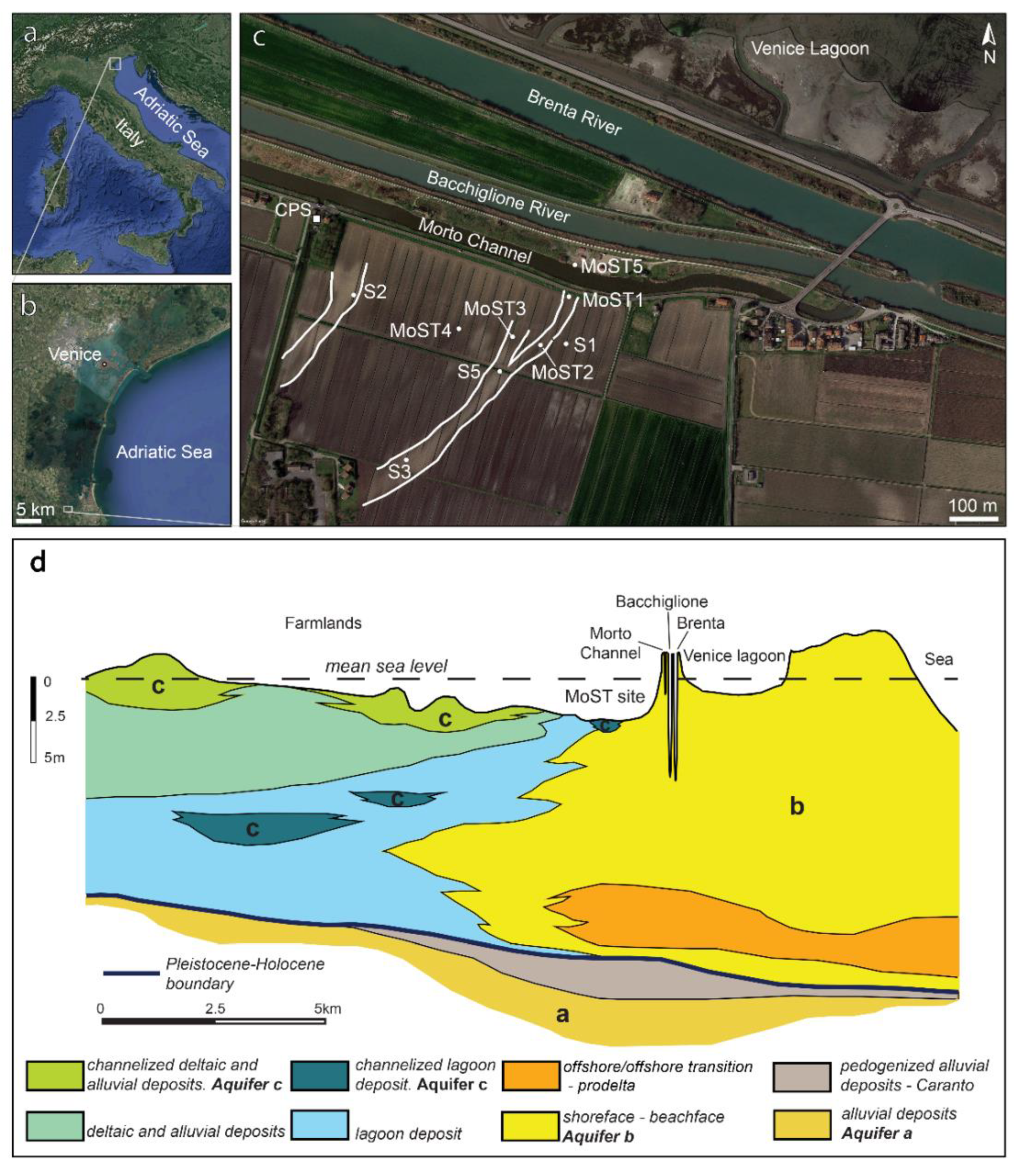
2. Study Area
3. Materials and Methods
4. Results
4.1. Facies Associations and Hydrostratigraphic Units
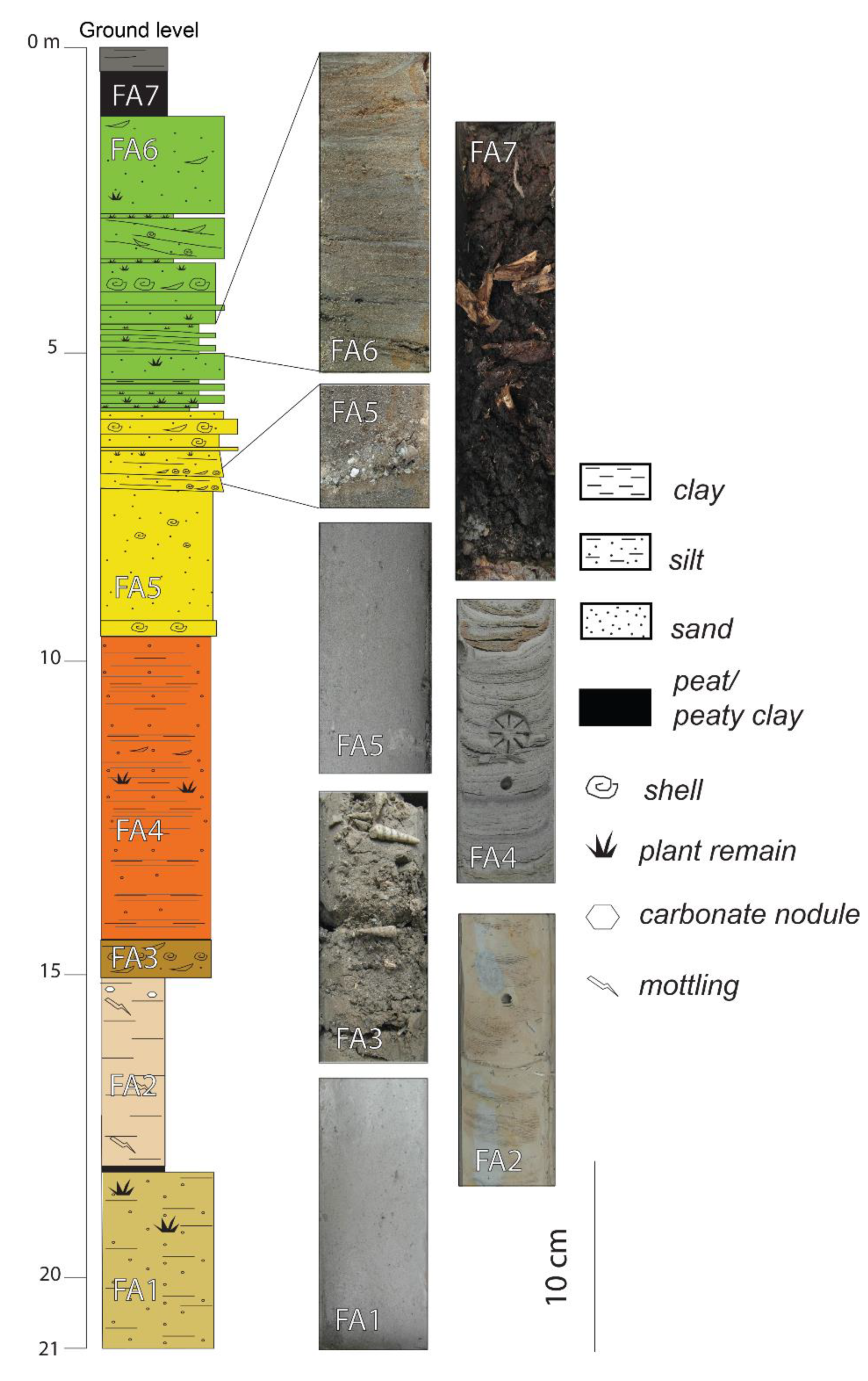
- Facies association one (FA1) exceeds 3 m in thickness and occurs in the lowest part of the study cores. It is formed by brownish–grayish sandy silt, locally presenting sub-horizontal to inclined millimetric lamination, vegetal remains and roots. These sedimentological features, together with data from previous studies [36,40,41,46] allow for attributing FA1 to the alluvial environment occurred in the area during the Last Glacial Maximum. From a hydrogeologic perspective, this facies association (HU1) represents the uppermost surficial confined aquifer (described in literature) [40,41,47] hosted in the Pleistocene continental deposits and confined at the top by the caranto paleosol.
- Facies association two (FA2) is 3–4 m thick and consists of light brown clay to silty clay layers showing evident signs of pedogenesis, such as mottling and caliche nodules. The top of FA2 is marked by a bioturbated erosional surface. This facies association refers to the over-consolidated caranto paleosol. Being composed of fine-grained sediments, the hydro-stratigraphic unit associated to FA2 corresponds to an aquiclude (HU2), confining at the top the aquifer represented by HU1.
- Facies association three (FA3), showing a thickness of about 1 m, unconformably overlies through an erosional surface FA2, and it is composed by poorly sorted, grey silt to silty sand structureless deposits. In the lower part, it contains 2 or 3 cm thick layers of medium to coarse sand showing a basal erosional surface with abundant shell fragments and shells of bivalves and gastropods. Coarse-grained sediments and shell lags suggest a high-energy coastal environment. The erosion surfaces are interpreted to be the result of wave ravinement that cut underlying deposits, in response to rapid beach–barrier migration [48,49]. The shell-rich layers correspond to a transgressive lag, and the overlying sand is attributed to the back-barrier to the shoreface environment. This facies association corresponds to a thin aquifer (HU3), which is the deepest part of the phreatic aquifer system of the area [40,41,46].
- Facies association four (FA4) is 3.5–5 m thick and gradually overlies FA3. It is composed by an alternation of millimetric to centimetric thick layers of grey silt and sandy silt. It shows planar to cross laminations, rare vegetal remains, cm-thick sandy layers with marine bivalves, gastropods and shell fragments, testifying the occurrence of sediment transport and deposition under variable energy such as that developing in an offshore/offshore-transitional, possibly a prodelta, environment [40,41]. Being that FA4 is mostly composed by silty sediments with medium to low permeability, the related hydro-stratigraphic unit four (HU4) represents a transition between very low aquifer permeability and aquitard.
- Facies association five (FA5) ranges in thickness between 8 and 10 m. It consists of yellowish-gray structureless sand with a fossiliferous layer at the base. Very well sorted, fine to medium sand, with abundant shells and shell fragments, dominates at the base, while fine to medium sand, moderately sorted, with rare shell fragments and vegetal remains dominates in the upper portion. In the middle portion of this facies association are locally present 1–2 m of silty sand to silty layers with vegetal remains and shells. FA5 is interpreted to be developed in shoreface to beachface environment [47]. The hydro-stratigraphic unit related to FA5 (HU5), being composed by sandy permeable deposits, represents a major part of the phreatic aquifer of the area [46,47].
- Facies association six (FA6) is laterally discontinuous and erosionally overlies Fa5. Its thickness ranges between 5 and 0.5 m. FA6 contains grey to yellow moderately sorted medium to fine sands, alternating with sandy, silty clay and clayey-silt horizontal laminae, locally showing shell fragments or vegetal remains at their bases. The upper portion of FA6 shows mottling and traces of oxidation. The base of FA6 depicts a lenticular geometry, often marked by the presence of a fine layer containing abundant vegetal remains. These sedimentological characteristics, together with the mollusk shells and foraminifera content, indicate a lagoon-littoral transitional environment characterized by active exchanges with the sea. FA6 refers to the infilling of lagoon paleochannels, whose lenticular shapes are often well recognizable by remote sensing imagery (Figure 1). The related hydro-stratigraphic unit (HU6) represents local thin aquifer lenses contained in the lenticular sandbodies. The base of this aquifer is often composed by silty sediments, separating it from the littoral sands of HU5.
- Facies association seven (FA7) refers to discontinuous deposits of the uppermost subsoil layer, immediately below the arable land. It shows a maximum thickness of 4 m. FA7 contains peat, peaty-clay layers or clay levels with abundant vegetal remains of the wetlands existing in the area before the hydraulic reclamation that was performed at the beginning of 20th century. The reduced thickness or the absence of these uppermost deposits is due to the subaerial oxidation of peats and the related geochemical land subsidence. Because of its low permeability, the related hydro-stratigraphic unit (HU7) is considered an impervious layer.
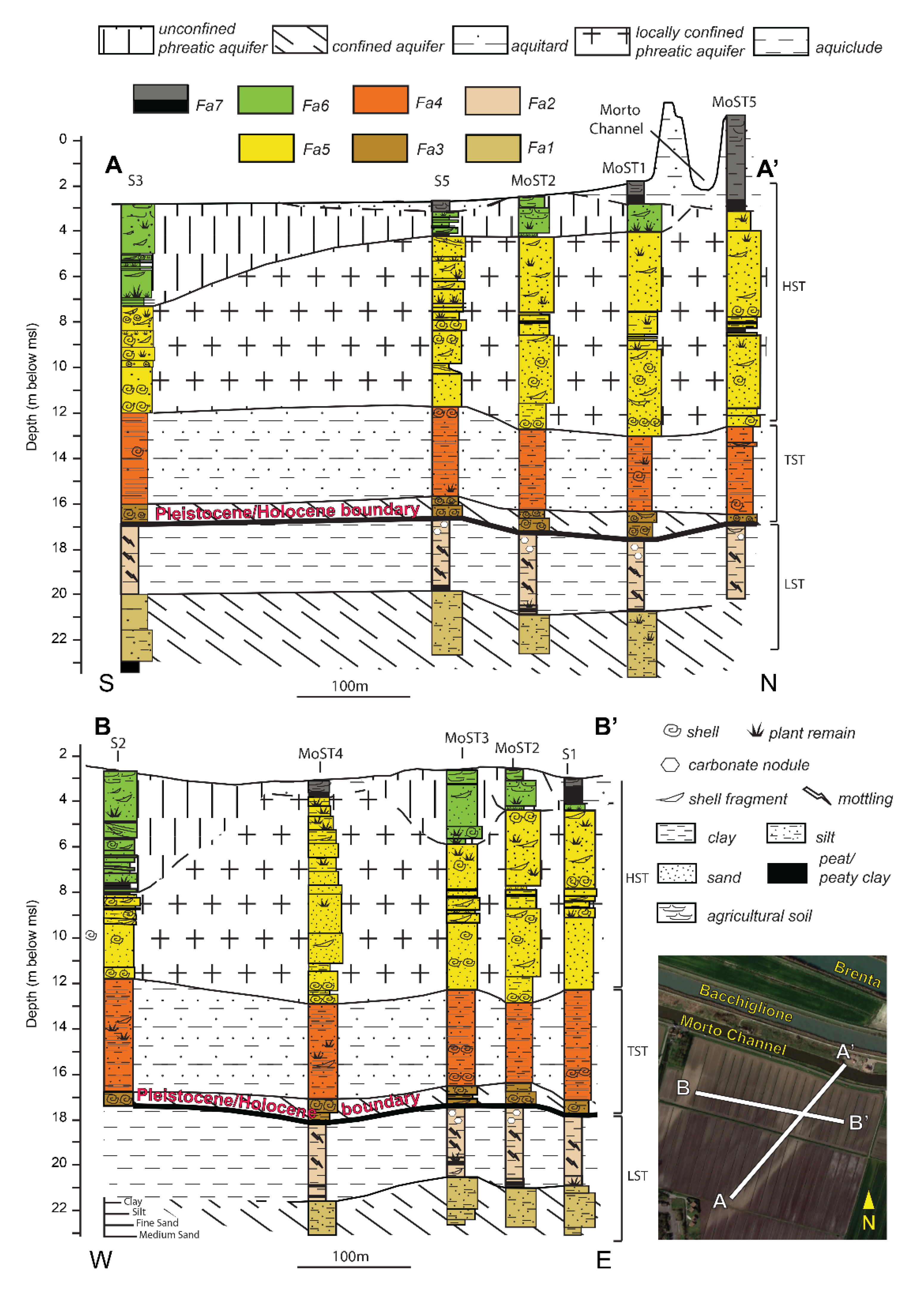
4.2. Hydrostratigraphic Model
4.3. Groundwater Dynamics
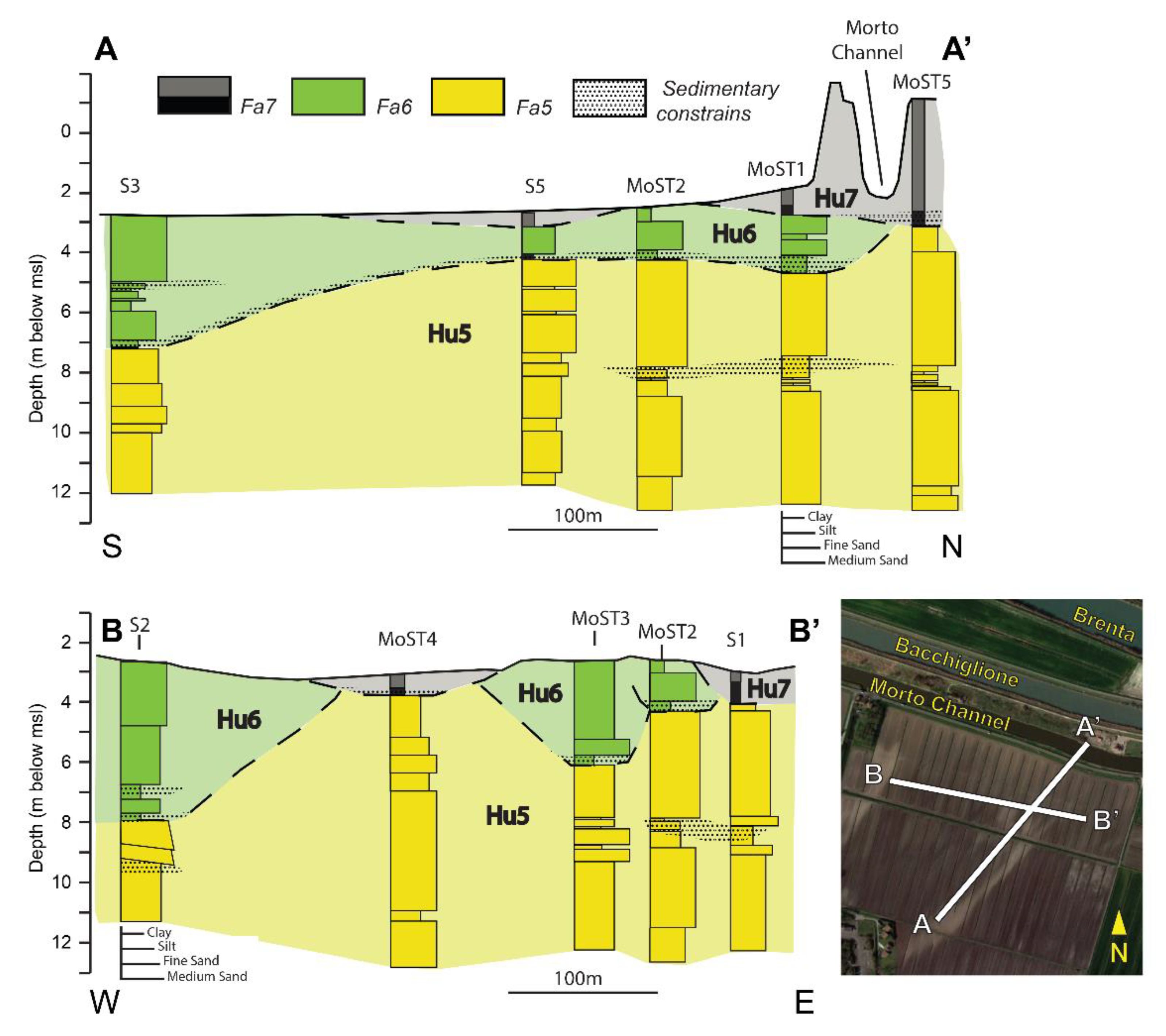
4.3.1. W-E Section
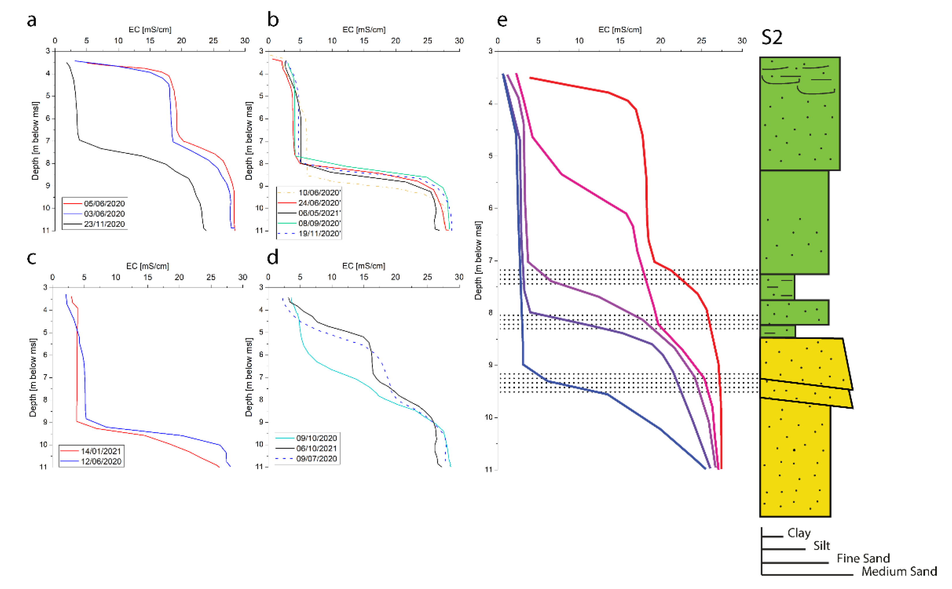
- S2: The EC values recorded in the water column of well S2 show a strong variability over the year, ranging between 2 and 30 mS/cm. The EC vertical profiles display the presence of a persistent freshwater lens floating over the salt-contaminated aquifer. The thickness of the freshwater lens varies from a few decimeters to about 5 m. Four main possible configurations of the fresh–saltwater interface have been recorded (Figure 4): (i) In the first configuration, the major change in EC is located at about 7 m below msl, in correspondence with a thin layer of silt inside the channelized aquifer (HU6). In one case, recorded on 11 November 2020, the aquifer presents 2–3 mS/cm down to this level; in the other two cases, recorded in Spring 2020, freshwater is present only in the first centimeters of the aquifer corresponding to the base of the agricultural soil; then the salinity rapidly increases, reaching 17–18 mS/cm at 4 m depth, and remains constant down to 7 m below msl, where the silty layer occurs in HU6. Below this level, the salinity rapidly increases, reaching its maximum value (28 mS/cm), and remains constant down to the bottom of the aquifer (Figure 4a). (ii) The second configuration is defined by a thicker freshwater lens (with EC values up to 5 mS/cm), which reaches the base of the channelized aquifer (HU6), at around 8 m below msl, where thin layers of silt occur (b). (iii) The third configuration is identified by a freshwater lens that reaches its maximum thickness down to 9 m below msl where a decrease in the grain size occurs within the sandy littoral aquifer (HU5) (Figure 4c). (iv) In the last configuration, the fresh–saltwater interface gradually deepens, representing transitional steps in the mitigation of the salt-contaminated aquifer, depending on the availability of freshwater (Figure 4d). Summarizing, the sedimentological constraints of the groundwater dynamics in well S2 lie at, 7 m, 8 m and 9 m below msl, influencing the depth of fresh–saltwater interface depending on the availability of freshwater in the aquifer. A freshwater lens is always present in this part of the aquifer, varying its depth roughly between 3.5 and 9 m below msl (Figure 4e).

- MoST4: The vertical EC profiles recorded in MoST4 well present values between 20 mS/cm and 30 mS/cm, from the top to the bottom of the aquifer. The EC does not show a strong vertical variability. A change in EC values is shown at the very top of the aquifer, where the curve shows a deflection to lower values (down to 20 mS/cm, Figure 5), in correspondence of a peaty clay layer at the top of the subsoil (HU7). The rest of the vertical profiles do not display other evidence of changes in salinity. The subsoil in this area is quite homogeneously composed by sand of the littoral aquifer (HU5). One stratigraphic constraint to the groundwater dynamics is at around 4 m below the msl, where a peat layer occurs (HU7) corresponding to the lower levels of EC at the top.

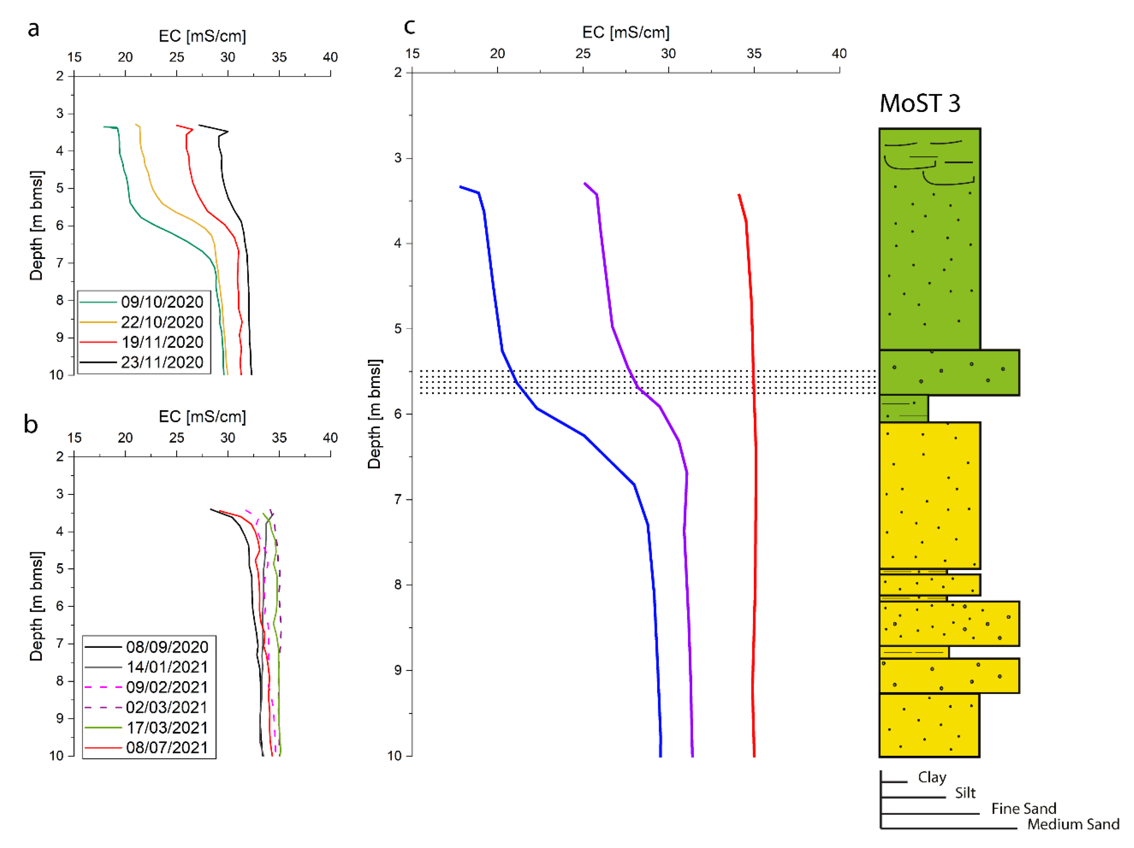
- MoST3: The EC values recorded in the water column of MoST3 well range between 18 mS/cm and 35 mS/cm. The EC shows a strong vertical variability identifying two possible configurations (Figure 6) of the fresh–saltwater interface through the year: (i) the first 2 m of the aquifer present a water lens with EC values variable between 18 and 30 mS/cm. The base of the lens is confined by a thin silty layer at the base of the channelized aquifer (HU6) at around 6 m below msl. Below this level EC values are higher varying between 28 and 32 mS/cm; (ii) the other profiles oscillate between 30 and 35 mS/cm without a vertical stratification. Summarizing, the stratigraphic constraint in MoST3 lies at 6 m below msl, periodically hosting a water lens whose EC values depend on the availability of freshwater.

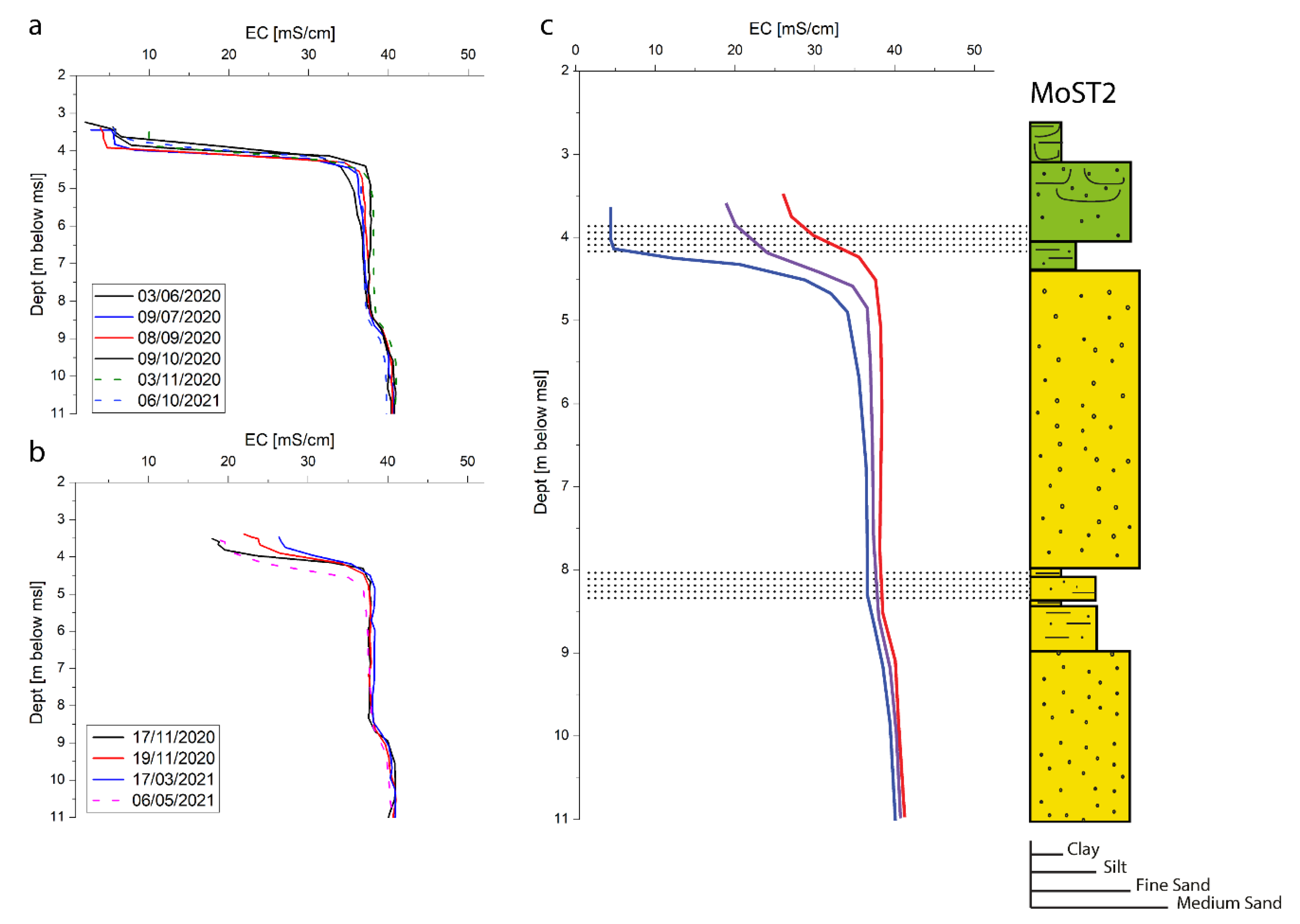
- MoST2: The EC profiles recorded in the groundwater of MoST2 well show a large vertical variability, between 2 and 42 mS/cm, while there is no significant change over the year except for the very upper part. The aquifer presents two possible configurations of the vertical EC curve: (i) lower EC values, between 2 and 5 mS/cm, are recorded in the first meter, down to 4 m below msl, corresponding to a thin layer of silty clay at the base of the channelized aquifer (HU6). Below this level, the salinity rapidly increases, reaching EC values of 35–38 mS/cm. These values remain constant down to around 8.5 m below msl. At this depth, corresponding to layers of silt and peaty clays in the littoral aquifer (HU5), the EC values increase again, reaching 40–42 mS/cm (Figure 7a) (ii) The major changes in salinity are located in the same position of the first configuration, but the EC values of the first meter never get below 17 mS/cm (Figure 7b). Summarizing the EC profiles outline the presence of two sedimentological constraints: the upper one (4 m below msl) corresponds to the base of the HU2, and the lower one corresponds to a thin clay layer in the littoral aquifer (HU5) at about 9 m in depth. The salinity of the first meter of the aquifer varies during the year, depending on the availability of freshwater (Figure 7c).

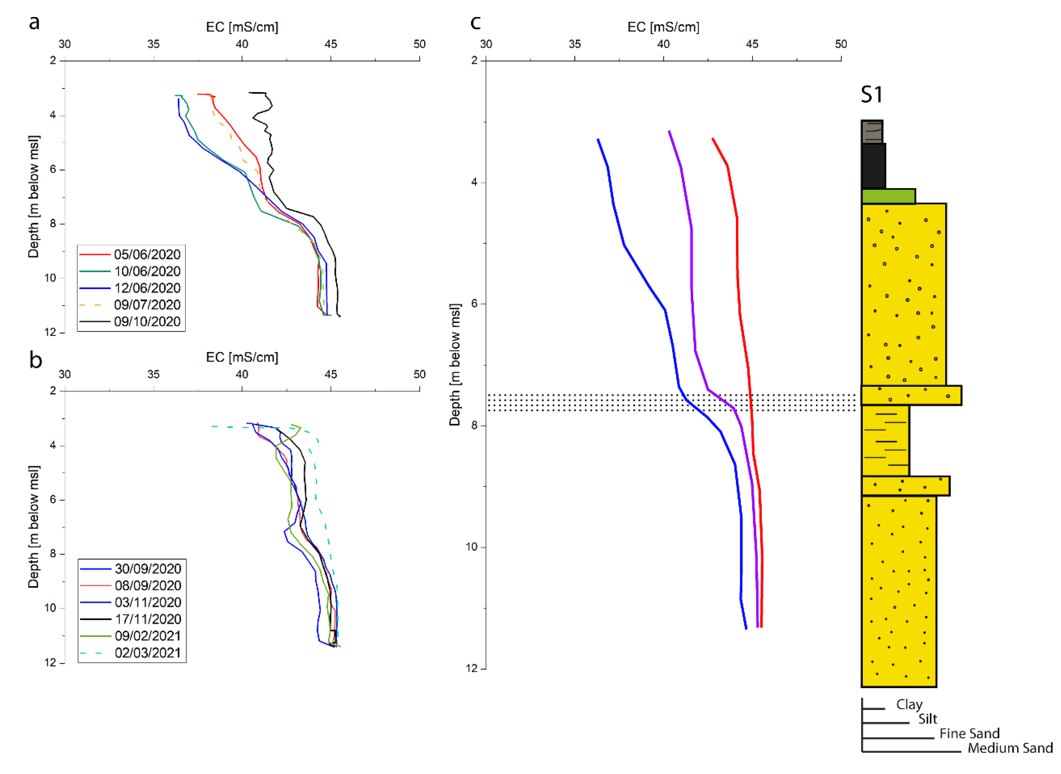
- S1: The vertical EC profiles recorded in the easternmost well (S1) display moderate vertical variability, with values ranging between 35 and 45 mS/cm, and low variability over the year, presenting two configurations (Figure 8): (i) the EC values vary between 35 and 42 down to about 8 m below msl, corresponding to a clayey silt layer in the littoral aquifer (HU5). Below this level the EC values reach 45 mS/cm and remain constant down to the bottom of the aquifer; (ii) the variability of salinity is very low, with values between 40 and 45 mS/cm throughout the whole thickness of the aquifer. Summarizing, even if the EC curve presents high values from the top to the bottom of the aquifer, the slight change in EC values in configuration (i) suggests the presence of a sedimentological constraint at around 8 m below msl. Above this level, the salinity of the aquifer could present slightly lower values depending on the availability of freshwater.

4.3.2. N-S Section
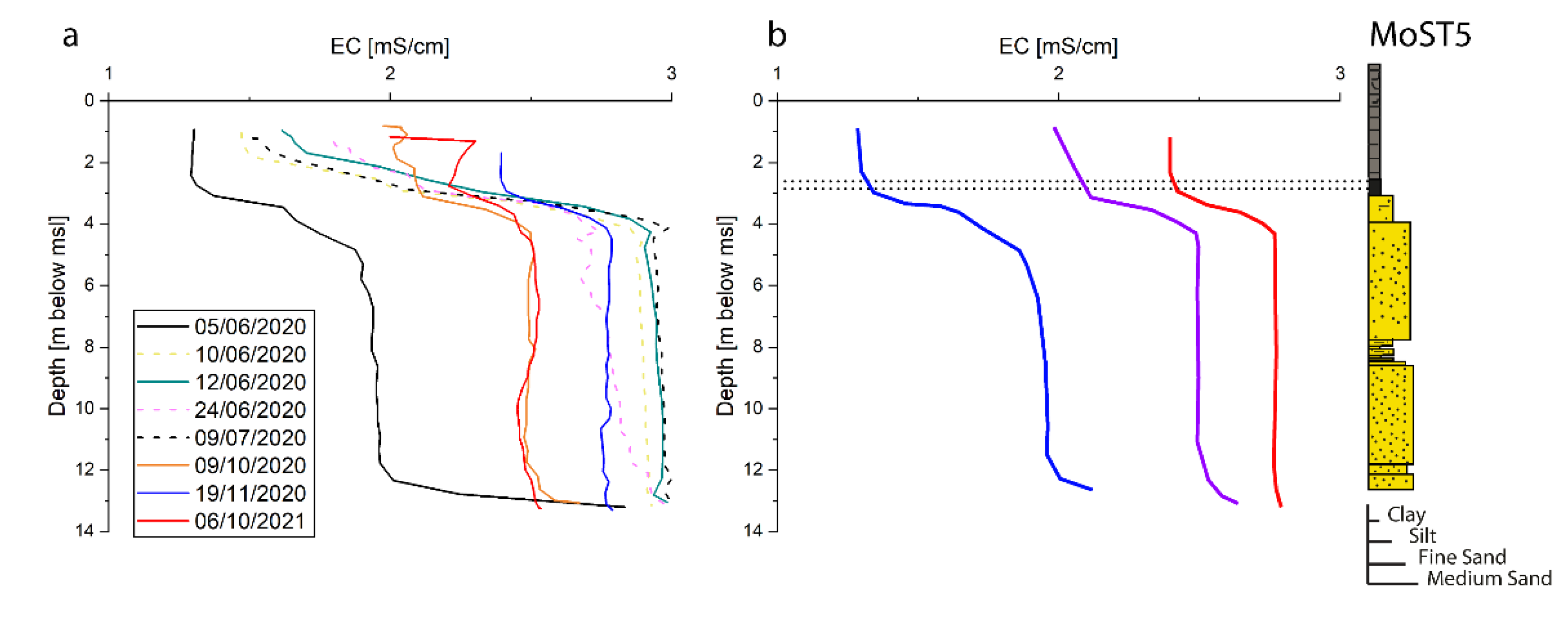
- MoST5: The northernmost well of the study area (MoST5) is located at the northern bank of the Morto Channel, and it is the only well of the studied network located over msl (1 m over msl). The vertical EC profiles present extremely low variability, being always fresh with values around 0.5–3 mS/cm from the top to the bottom, due to the seepage of freshwater from the Morto Channel. The recorded profiles (Figure 9a) show a small increase in the EC, from a minimum of 0.5 to a maximum of 3 mS/cm, at 3 m below msl, corresponding to a peaty clay layer at the base of HU1. Below the clay layer, the value remains constant, between 2 and 3 mS/cm, along the whole profile. The only stratigraphic constraint in this profile is located at 3 m below msl. Since the water is fresh and not stratified, no other sedimentological constraints can be found/identified.
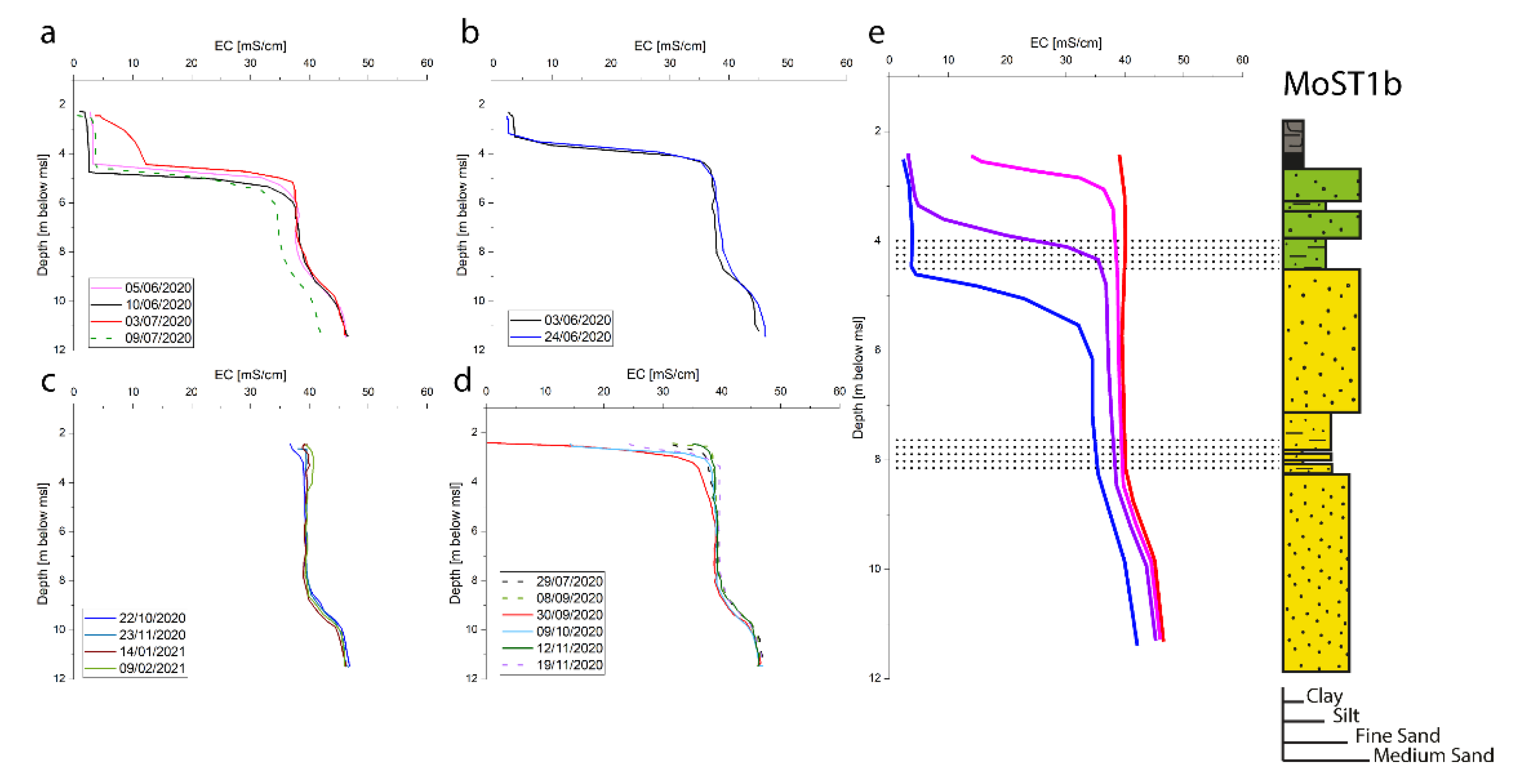
- MoST1: The EC recorded in MoST1 well indicates a very high vertical variability between 0 to 50 mS/cm in the upper 3 m and different behaviors over the year. Four different configurations of the fresh–saltwater interface are present (Figure 10): (i) in the first configuration a freshwater lens, 3 m thick, lays on a thin silty layer at 5 m below msl, corresponding to the base of the local channelized aquifer (HU6). Below this level, the salinity rapidly increases, reaching values between 33 and 40 mS/cm; (ii) the second configuration does not show a vertical stratification in the upper part, presenting an EC value of about 40 mS/cm; (iii) and (iv) configurations represent intermediate conditions in the fresh–saltwater dynamics of the upper part of the aquifer, possibly also influenced by the presence of minor sedimentological constraints: a thin silty layer inside HU2, for the third one, and a surficial peat layer at 2–2.5 m for the fourth one. In all the configurations, the EC profiles show a change at about 9 m below msl, where thin fine layers occur inside the littoral aquifer (HU5). Below this level the EC reaches its maximum value (45–48 mS/cm). Summarizing, two main sedimentological constraints were identified at around 5 and 9 m below msl. In the first 3 m of the aquifer, a freshwater lens is often present, with variable thickness depending on the freshwater availability.
- MoST2: see in the previous section
- S5: The EC recorded in the S5 well shows low vertical and seasonal variability, with values ranging between 21 and 27 mS/cm. Two configurations are recognized (Figure 11): (i) in the first configuration, the first 1–1.5 m, corresponding to the channelized aquifer (HU6) presents lower EC values. Below 5 m depth, the profiles remain constant around 26 mS/cm; (ii) the other EC recorded in S5 well present a vertical constant profile, with values around 26 mS/cm. Summarizing, the fine layer at the base of the channelized aquifer (HU6) represents the only stratigraphic constraint of the groundwater dynamics in this portion of the aquifer.
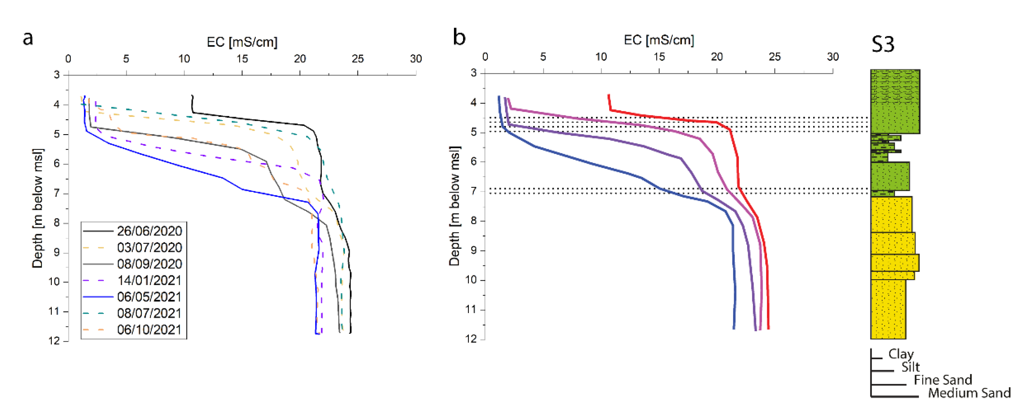
- S3: The EC profiles recorded in S3 well presents a high vertical variability, with values between 0 to 25 mS/cm (Figure 12). The lower portion is constantly between 20 and 25 mS/cm, while the upper 6–7 m present a strong variability over the year, with a surficial freshwater lens confined between the base of the agricultural soil and silty layers inside the local channelized aquifer (HU6, Figure 1). Within this range, the fresh–saltwater interface can assume intermediate configurations with fresher water lens with various thicknesses over the year. Below 2 m depth (5 m below msl), the EC rapidly increases reaching 20–25 mS/cm at the top of the littoral aquifer (HU5). Roughly between 5 and 7 m below msl, the groundwater can present different salinities, depending on the availability of freshwater, never exceeding 20–22 mS/cm. Another change in EC is found at about 7 m below msl, where a silty layer at the base of HU2 confines relatively fresher water. Below this level, the EC reaches its maximum values, between 22 and 25 mS/cm, and remains constant down to the bottom of the aquifer. Summarizing, the phreatic aquifer in this area present two main stratigraphic constraints, at 5 and 7 m below msl, respectively, corresponding to fine sedimentological layers inside the HU6.
5. Discussion
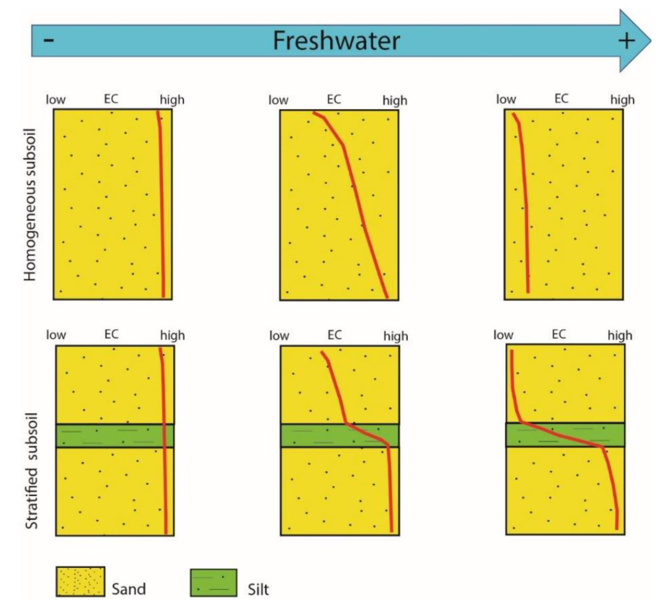
5.1. Fresh–Saltwater Dynamic Model
5.2. Stratigraphic Constraints in N-S and W-E Sections
- At the base of Hu6, where clay and silty layers are present. The presence of the channelized aquifers triggers the formation and the maintenance through time of fresher water lenses in the phreatic aquifer. This occurs homogeneously along the N-S section, corresponding to a N-S directed paleochannel, and in correspondence of MoST2, MoST3 and S2 points, in the W-E section.
- At the top of clay and silty layers in Hu6. This occurs in the western channelized surficial sandbody (observed in S2 point) and in the southern part of the eastern one (observed in S3 point), where the channelized aquifers (Hu6) show their major thickness.
- In the upper part of the littoral aquifer Hu5 where coarser sand grades downward to finer sand (as in S2 point).
- Around the middle portion of Hu5, where silty-clay layers occur (in S1, MoST1 and MoST2 points).
- At the base of Hu7, in correspondence to peaty clay layers that could preserve fresher water at the very top of the phreatic aquifer (as it was observed in MoST5 and MoST4 points).
5.3. Fresh–Saltwater Dynamics in Best and Worst Mitigation Condition
5.3.1. N-S Section (Figure 15a)
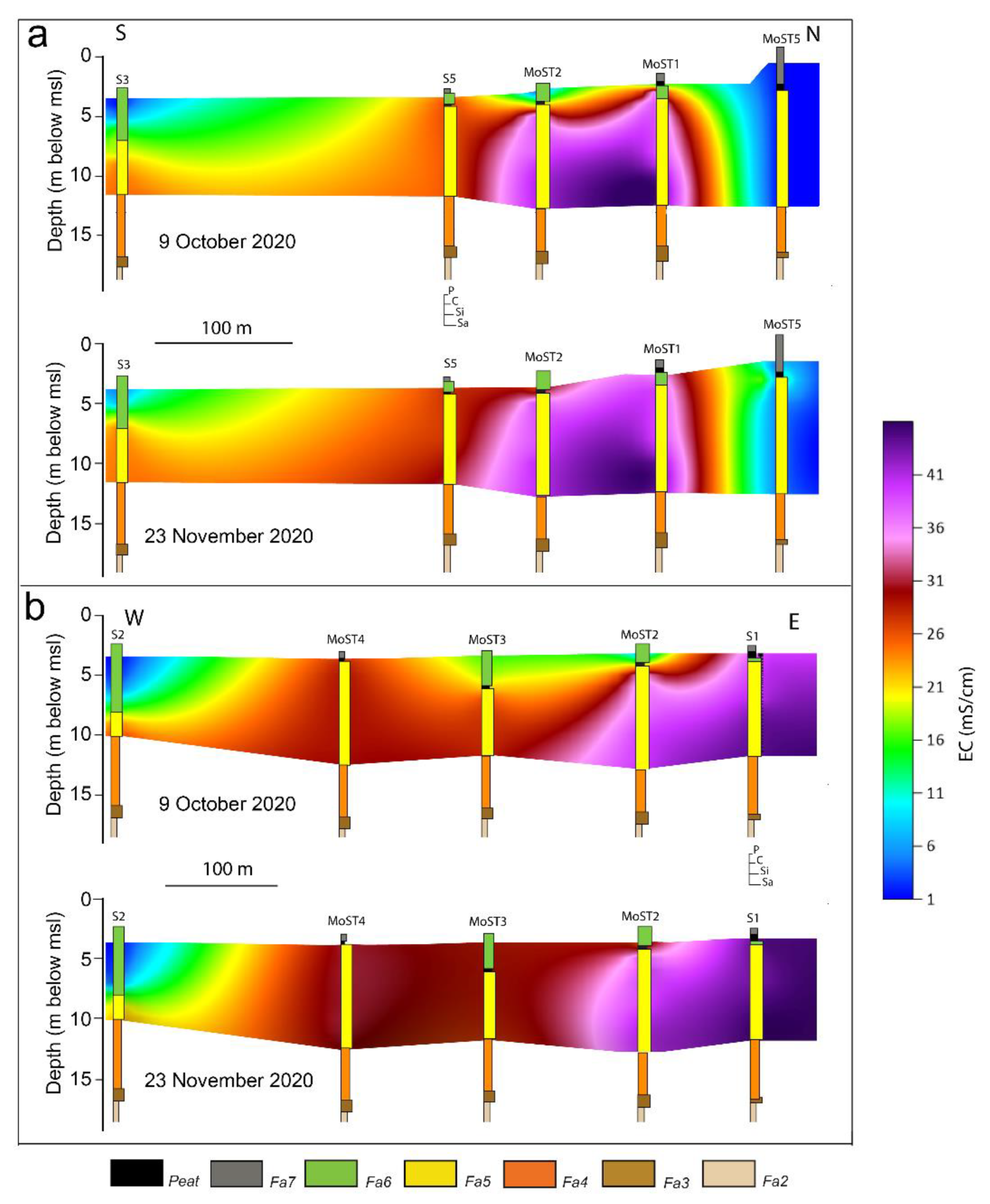
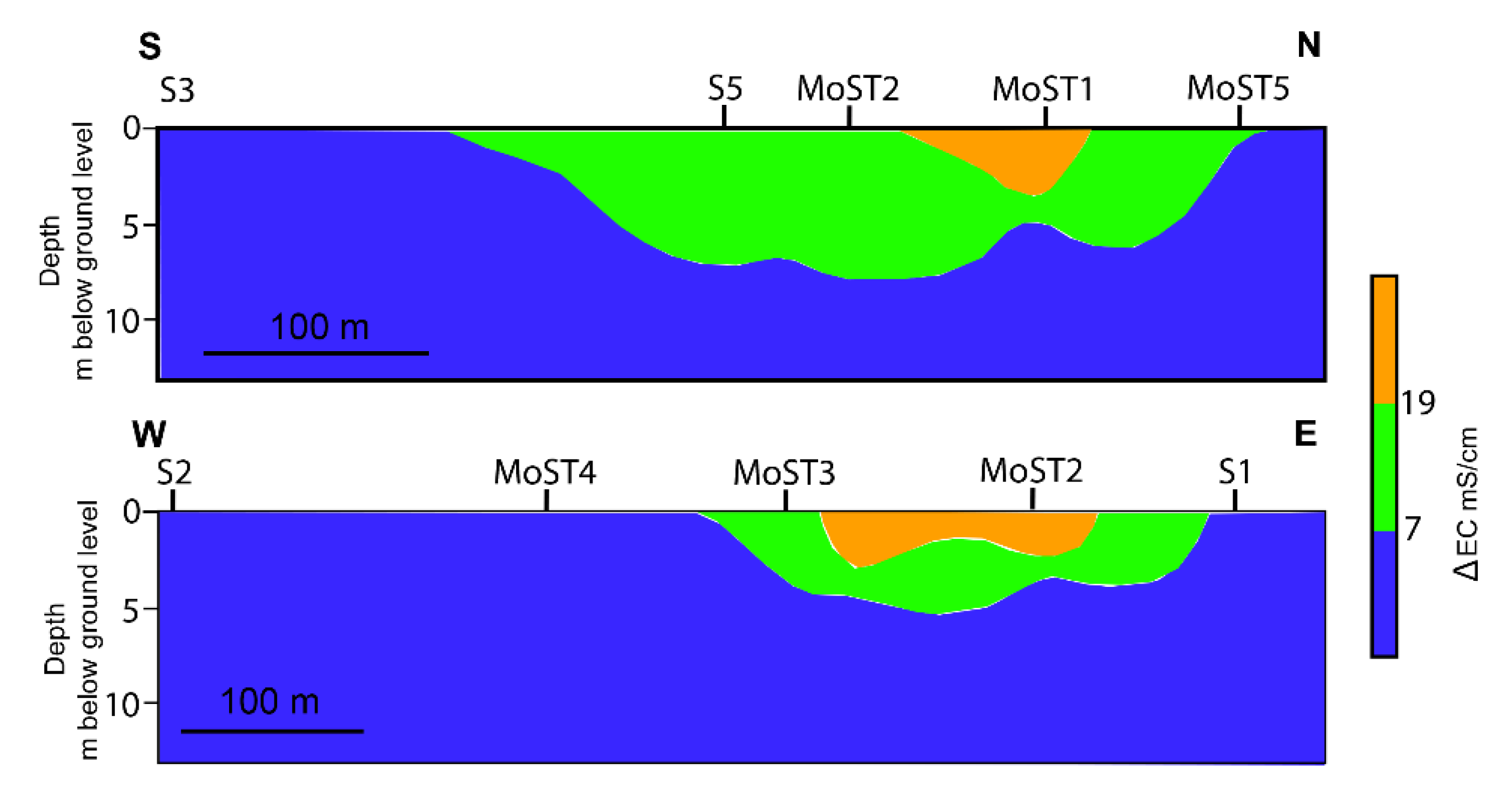
- Best mitigation conditions: the EC of the aquifer is characterized by the presence of an extended salty bulge in the middle part of the area, recorded in MoST1 and MoST2, featuring an EC higher than 35 mS/cm and reaching the depth of around 5 m below sea level. The top of the aquifer, in this area, is characterized by the presence of a fresher water lens up to 1–2 m. To the north, the EC strongly decreases, and the aquifer results fresh from the bottom to the top (MoST5), due to the presence of the Morto Channel, whose freshwater seeping from the channel bed infiltrates into the subsoil. To the south, the deep portion of the aquifer is still salty, around 20–25 mS/cm, while it freshens towards the top, where a freshwater lens up to a depth of 5 m is present (S2).
- Worst mitigation conditions: the saltwater bulge in the middle portion of the aquifer reaches the surface, the fresher water lens disappears. The freshwater lens in the southern portion of the area (S3) is still present, even if it is smaller and the EC values are higher.

5.3.2. W-E Section (Figure 15b)
- Best mitigation conditions: the eastern part of the area shows the highest EC levels (35–40 mS/cm, from bottom to the top in S1 well) and presents a fresher water lens in the MoST2 well. Moving to the west the surficial lens is present also in MoST3 well with EC values down to 15 ms/cm, where the deepest part reaches EC values of about 25–30 mS/cm. In the western part, the upper aquifer presents a freshwater lens extending for a width of about 10 m and a thickness of 7–8 m.
- Worst mitigation conditions: the surficial freshwater lenses disappear except for the western one that only decreases its overall extension.
6. Conclusions
- We demonstrated that the groundwater dynamics is influenced by sedimentological constraints.
- The constraints correspond to: peat layers at the base of Hu7, fine-grained layers inside Hu6 or at its base, and the transition between finer and coarser sand in Hu3.
- In the phreatic aquifer we recognized three possible groundwater dynamics conditions: (i) in the westernmost and southernmost portions a thick freshwater lens is always present. The lenses are confined at the top of the aquifer by stratigraphic constraints located at different depths, depending on the amount of precipitation. This condition occurs where the Hu6 is thicker and Hu7 is absent; (ii) in the central-northern part of the area, a fresher water lens could develop in the most surficial part when the availability of freshwater allows the formation of the lens (MoST1, MoST2, MoST3). The lenses are confined at the base by the stratigraphic constraint at the base of Hu6. This condition occurs where the Hu6 is present and Hu7 is absent (except for MoST1 that possibly receives freshwater inputs from the Morto Channel); (iii) in the other areas, where Hu7 is present and Hu6 is absent (S1, S5, MoST4, MoST5), freshwater lenses never develop, and the aquifer is always salty (except for the MoST5 site that receives freshwater from the Morto Channel and the aquifer is always fresh). In these areas, the stratigraphic constraints are barely recognizable and separate waters with similar EC.
- The portion of the aquifer most influenced by freshwater availability is the north-central part, where a paleochannel system (Hu6) is present, but with minor thickness than at the westernmost and southernmost part of the area. This area, being the most sensitive to changes in freshwater inputs, should be considered in the framework of eventual mitigation strategies.
- We demonstrated the importance of a detailed reconstruction of the subsoil architecture in order to understand the stratigraphic influence on the fresh–saltwater dynamics into the aquifers. Thus, a detailed sedimentological analysis is critical to optimize water management in highly salinized aquifer systems.
- A detailed analysis of the geological—geomorphological variations resulting from the Holocene evolution of the coastal zones, along with hydrogeological analyses, are basic/fundamental tools for the exploration of freshwater lenses in coastal areas.
Author Contributions
Funding
Institutional Review Board Statement
Informed Consent Statement
Data Availability Statement
Conflicts of Interest
References
- Rasmussen, P.; Sonnenborg, T.O.; Goncear, G.; Hinsby, K. Assessing impacts of climate change, sea level rise, and drainage canals on saltwater intrusion to coastal aquifer. Hydrol. Earth Syst. Sci. 2013, 17, 421–443. [Google Scholar] [CrossRef]
- Mastrocicco, M.; Colomani, N. The Issue of Groundwater Salinization in Coastal Areas of the Mediterranean Region: A Review. Water 2021, 13, 90. [Google Scholar] [CrossRef]
- Hussain, M.S.; Abd-Elhamid, H.F.; Javadi, A.A.; Sherif, M.M. Management of Seawater Intrusion in Coastal Aquifers: A Review. Water 2019, 11, 2467. [Google Scholar] [CrossRef]
- Johnson, T.A.; Whitaker, R. Saltwater Intrusion in the Coastal Aquifers of Los Angeles County, California: Coastal Aquifer Management; Cheng, A., Ouazar, D., Eds.; Lewis: Boca Raton, FL, USA, 2004. [Google Scholar]
- Edington, D.; Poeter, E. Stratigraphic Control of Flow and Transport Characteristics. Ground Water 2006, 44, 826–831. [Google Scholar] [CrossRef] [PubMed]
- Sugarman, P.J.; Miller, K.G. Correlation of Miocene Sequences and Hydrogeologic Units, New Jersey Coastal Plain. Sed. Geol. 1997, 108, 3–18. [Google Scholar] [CrossRef]
- Campo, B.; Bohacs, K.M.; Amorosi, A. Late quaternary sequence stratigraphy as a tool for groundwater exploration: Lessons from the Po River Basin (northern Italy). AAPG Bull. 2020, 104, 681–710. [Google Scholar] [CrossRef]
- Fogg, G.E.; Noyes, C.D.; Carle, S.F. Geologically based model of heterogeneous hydraulic conductivity in an alluvial setting. Hydrogeol. J. 1998, 6, 131–143. [Google Scholar] [CrossRef]
- Weissmann, G.S.; Carle, S.F.; Fogg, G.E. Three-dimensional hydrofacies modeling based on soil surveys and transition probability geostatistics. Water Resour. Res. 1999, 35, 1761–1770. [Google Scholar] [CrossRef]
- Hornung, J.; Aigner, T. Reservoir and aquifer characterization of fluvial architectural elements: Stubensandstein, Upper Triassic, southwest Germany. Sed. Geol. 1999, 129, 215–280. [Google Scholar] [CrossRef]
- Zappa, G.; Bersezio, R.; Felletti, F.; Giudici, M. Modeling heterogeneity of gravel-sand, braided stream, alluvial aquifers at the facies scale. J. Hydrol. 2006, 325, 134–153. [Google Scholar] [CrossRef]
- Van Dijk, W.M.; Densmore, A.L.; Sinha, R.; Singh, A. Reduced-complexity probabilistic reconstruction of alluvial aquifer stratigraphy, and application to sedimentary fans in northwestern India. J. Hydrol. 2016, 541, 1241–1257. [Google Scholar] [CrossRef]
- Heinz, J.; Kleineidam, S.; Teutsch, G.; Aigner, T. Heterogeneity patterns of quaternary glaciofluvial gravel bodies (SW-Germany): Application to hydrogeology. Sed. Geol. 2003, 158, 1–23. [Google Scholar] [CrossRef]
- Vassena, C.; Cattaneo, L.; Giudici, M. Assessment of the role of facies heterogeneity at the fine scale by numerical transport experiments and connectivity indicators. Hydrogeol. J. 2010, 18, 651–668. [Google Scholar] [CrossRef]
- Berg, S.J.; Illman, W.A. Capturing aquifer heterogeneity: Comparison of approaches through controlled sandbox experiments. Water Resour. Res. 2011, 47, W09514. [Google Scholar] [CrossRef]
- Bianchi, M.; Kearsey, T.; Kingdon, A. Integrating deterministic lithostratigraphic models in stochastic realizations of subsurface heterogeneity. Impact on predictions of lithology, hydraulic heads and groundwater fluxes. J. Hydrol. 2015, 531, 557–573. [Google Scholar] [CrossRef]
- Maples, S.R.; Foglia, L.; Fogg, G.E.; Maxwell, R.M. Sensitivity of hydrologic and geologic parameters on recharge processes in a highly heterogeneous, semi-confined aquifer system. Hydrol. Earth Syst. Sci. 2020, 24, 2437–2456. [Google Scholar] [CrossRef]
- Jordan, D.W.; Pryor, W.A. Hierarchical Levels of Heterogeneity in a Mississippi River Meander Belt and Application to Reservoir Systems: Geologic Note. AAPG Bull. 1992, 76, 1601–1624. [Google Scholar] [CrossRef]
- Damico, J.R.; Ritzi, R.W.; Gershenzon, N.I.; Okwen, R.T. Challenging Geostatistical Methods to Represent Heterogeneity in CO2 Reservoirs under Residual Trapping. Environ. Eng. Geosci. 2018, 24, 357–373. [Google Scholar] [CrossRef]
- Carol, E.; Cellone, F.; Tanjal, C.; Galliari, M.J. Role of the geologic-geomorphic setting of the Río de la Plata estuary coastal landscape in controlling freshwater lenses shape and distribution. J. South Am. Earth Sci. 2022, 116, 103832. [Google Scholar] [CrossRef]
- Maas, E.; Grattan, S.R. Crop Yields as Affected by Salinity. In Agricultural Drainage; Skaggs, R.W., van Schilfgaarde, J., Eds.; Wiley: New York, NY, USA, 1999; pp. 55–108. [Google Scholar] [CrossRef]
- Carbognin, L.; Gambolati, G.; Putti, M.; Rizzetto, F.; Teatini, P. Soil contamination and land subsidence raise concern in the Venice watershed, Italy. WIT Trans. Ecol. Environ. 2006, 99, 691–700. [Google Scholar] [CrossRef]
- Carbognin, L.; Teatini, P.; Tosi, L. The Impact of Relative Sea Level Rise on the Northern Adriatic Sea Coast, Italy. WIT Trans. Ecol. Environ. 2009, 127, 137–148. [Google Scholar] [CrossRef]
- Carbognin, L.; Teatini, P.; Tomasin, A.; Tosi, L. Global change and relative sea level rise at Venice: What impact in term of flooding. Clim. Dyn. 2010, 35, 1039–1047. [Google Scholar] [CrossRef]
- Carbognin, L.; Tosi, L. Il Progetto ISES per L’analisi dei Processi di Intrusione Salina e Subsidenza Nei Territori Meridionali Delle Provincie di Padova e Venezia. Consiglio Nazionale delle Ricerche, Istituto per lo Studio della Dinamica delle Grandi Masse: Venice, Italy, 2003. [Google Scholar]
- De Franco, R.; Biella, G.; Tosi, L.; Teatini, P.; Lozej, A.; Chiozzotto, B.; Giada, M.; Rizzetto, F. Monitoring the saltwater intrusion by time lapse electrical resistivity tomography: The Chioggia test site (Venice Lagoon, Italy). J. Appl. Geophys. 2009, 69, 117–130. [Google Scholar] [CrossRef]
- Gattacceca, J.C.; Vallet-Coulomb, C.; Mayer, A.; Claude, C.; Radakovitch, O.; Conchetto, E.; Hamelin, B. Isotopic and geochemical characterization of salinization in the shallow aquifers of a reclaimed subsiding zone: The southern Venice Lagoon coastland. J. Hydrol. 2009, 378, 46–61. [Google Scholar] [CrossRef]
- Gattacceca, J.C.; Mayer, A.; Cucco, A.; Claude, C.; Radakovitch, O.; Vallet-Coulomb, C.; Hamelin, B. Submarine groundwater discharge in a subsiding coastal lowland: A 226Ra and 222Rn investigation in the Southern Venice lagoon. Appl. Geochem. 2011, 26, 907–920. [Google Scholar] [CrossRef]
- Viezzoli, A.; Tosi, L.; Teatini, P.; Silvestri, S. Surface water-groundwater exchange in transitional coastal environments by airborne electromagnetics: The Venice Lagoon example. Geophys. Res. Lett. 2010, 37, L01402. [Google Scholar] [CrossRef]
- Teatini, P.; Tosi, L.; Viezzoli, A.; Baradello, L.; Zecchin, M.; Silvestri, S. Understanding the hydrogeology of the Venice Lagoon subsurface with airborne electromagnetics. J. Hydrol. 2011, 411, 342–354. [Google Scholar] [CrossRef]
- Tosi, L.; Baradello, L.; Teatini, P.; Zecchin, M.; Bonardi, M.; Shi, P.; Tang, C.; Li, F.; Brancolini, G.; Chen, Q.; et al. Combined continuous electrical tomography and very high resolution seismic surveys to assess continental and marine groundwater mixing. Boll. Geofis. Teor. Ed. Appl. 2011, 52, 585–594. [Google Scholar]
- Da Lio, C.; Carol, E.; Kruse, E.; Teatini, P.; Tosi, L. Saltwater contamination in the managed low-lying farmland of the Venice coast, Italy: An assessment of vulnerability. Sci. Total Environ. 2015, 533, 356–369. [Google Scholar] [CrossRef] [PubMed]
- Tosi, L.; Da Lio, C.; Bergamasco, A.; Cosma, M.; Cavallina, C.; Fasson, A.; Viezzoli, A.; Zaggia, L.; Donnici, S. Sensitivity, Hazard, and Vulnerability of Farmlands to Saltwater Intrusion in Low-Lying Coastal Areas of Venice, Italy. Water 2022, 14, 64. [Google Scholar] [CrossRef]
- Lovrinović, I.; Bergamasco, A.; Srzić, V.; Cavallina, C.; Holjević, D.; Donnici, S.; Erceg, J.; Zaggia, L.; Tosi, L. Groundwater monitoring systems to understand sea water intrusion dynamics in the Mediterranean: The Neretva valley and the southern Venice coastal aquifers case studies. Water 2021, 13, 561. [Google Scholar] [CrossRef]
- Rizzetto, F.; Tosi, L.; Carbognin, L.; Bonardi, M. Geomorphic setting and related hydrogeological implications of the coastal plain south of the Venice Lagoon, Italy. In Hydrology of the Mediterranean and Semiardi Regions (Proceedings of an International Symposium Held at Montpellier. April 2003); No. 278; International Assn of Hydrological Sciences: Wallingford, UK, 2003. [Google Scholar]
- Zecchin, M.; Brancolini, G.; Tosi, L.; Rizzetto, F.; Caffau, M.; Baradello, L. Anatomy of the Holocene succession of the southern Venice lagoon revealed by very high-resolution seismic data. Cont. Shelf Res. 2009, 29, 1343–1359. [Google Scholar] [CrossRef]
- Storms, J.E.A.; Weltje, G.J.; Terra, G.J.; Cattaneo, A.; Trincardi, F. Coastal dynamics under conditions of rapid sea-level rise: Late Pleistocene to Early Holocene evolution of barrier–Lagoon systems on the northern Adriatic shelf (Italy). Quat. Sci. Rev. 2008, 27, 1107–1123. [Google Scholar] [CrossRef]
- Mozzi, P.; Bini, C.; Zilocchi, L.; Becattini, R.; Mariotti Lippi, M. Stratigraphy, palaeopedology and palynology of late Pleistocene and Holocene deposits in the landward sector of the Lagoon of Venice (Italy), in relation to the Caranto level. Ital. J. Quat. Sci. 2003, 16(1bis), 193–210. [Google Scholar]
- Donnici, S.; Serandrei-Barbero, R.; Bini, C.; Bonardi, M.; Lezziero, A. The Caranto Paleosol and Its Role in the Early Urbanization of Venice. Geoarchaeology 2011, 26, 514–543. [Google Scholar] [CrossRef]
- Tosi, L.; Rizzetto, F.; Bonardi, M.; Donnici, S.; Serandrei-Barbero, R.; Toffoletto, F. Note Illustrative della Carta Geologica d’Italia alla Scala 1:50.000. Foglio 148–149; Chioggia-Malamocco; APAT, Dip. Difesa del Suolo, Servizio Geologico d’Italia, SystemCart: Rome, Italy, 2007; p. 164, 2 Maps. [Google Scholar]
- Tosi, L.; Rizzetto, F.; Zecchin, M.; Brancolini, G.; Baradello, L. Morphostratigraphic framework of the Venice Lagoon (Italy) by very shallow water VHRS surveys: Evidence of radical changes triggered by human-induced river diversions. Geophys. Res. Lett. 2009, 36, L09406. [Google Scholar] [CrossRef]
- Tosi, L.; Rizzetto, F.; Bonardi, M.; Donnici, S.; Serandrei-Barbero, R.; Toffoletto, F. Note Illustrative della Carta Geologica d’Italia alla Scala 1:50.000. Foglio 128; APAT, Dip. Difesa del Suolo, Servizio Geologico d’Italia, SystemCart: Rome, Italy, 2007; p. 164, 2 Maps. [Google Scholar]
- Bondesan, A.; Meneghel, M.; Rosselli, R.; Vitturi, A. Carta Geomorfologica Della Provincia di Venezia, Scala 1:50.000 (con edizione digitale alla scala 1:20.000); LAC: Firenze, Italy, 2004. [Google Scholar]
- Dalrymple, R.W. Interpreting sedimentary successions: Facies, facies analysis and facies models. In Facies Models 4; James, N.P., Dalrymple, R.W., Eds.; Geological Association of Canada: St. John, NL, Canada, 2010. [Google Scholar]
- Pszonka, J.; Schulz, B.; Sala, D. 2021: Application of mineral liberation analysis (MLA) for investigations of grain size distribution in submarine density flow deposits. Mar. Pet. Geol. 2021, 129, 105–109. [Google Scholar] [CrossRef]
- Vitturi, A.; Bassan, V.; Mazzuccato, A.; Primon, S.; Bondesan, A.; Ronchese, F.; Zangheri, P. Atlante Geologico della Provincia di Venezia; Note Illustrative; Arti Grafiche Venete: Venice, Italy, 2011. [Google Scholar]
- Fabbri, P.; Zangheri, P.; Bassan, V.; Fagarazzi, E.; Mazzuccato, A.; Primon, S.; Zogno, C. Sistemi idrogeologici della Provincia di Venezia; Provincia di Venezia, Servizio Geologico, Difesa del Suolo e Tutela del Territorio: Venice, Italy, 2013. [Google Scholar]
- Swift, D.J.P. Coastal Erosion and Transgressive Stratigraphy. J. Geol. 1969, 4, 444–456. [Google Scholar] [CrossRef]
- Nummedal, D.; Swift, D.J.P. Transgressive Stratigraphy at Sequence-Bounding Unconformities: Some Principles Derived from Holocene and Cretaceous Examples. In Sea-Level Fluctuation and Coastal Evolution; Nummedal, D., Pilkey, O.H., Howard, J.D., Eds.; SEPM Society for Sedimentary Geology; Special Publication 41; Tulsa, OK, USA, 1987. [Google Scholar] [CrossRef]
- Zecchin, M.; Baradello, L.; Brancolini, G.; Donda, F.; Rizzetto, F.; Tosi, L. Sequence stratigraphy based on high-resolution seismic profiles in the late Pleistocene and Holocene deposits of the Venice area. Mar. Geol. 2008, 253, 185–198. [Google Scholar] [CrossRef]
- Jichao, S.; Yuefei, H. Modeling the Simultaneous Effects of Particle Size and Porosity in Simulating Geo-Materials. Materials 2022, 15, 1576. [Google Scholar] [CrossRef]


| Aquifer System unit | Facies Association | Hydro-Stratigraphic Unit | Seismic Units by [36,41] | Sequence Stratigraphy from [36,41] |
|---|---|---|---|---|
| Phreatic aquifer | Fa7 (4 m below msl—core top) | Hu7: Peat and peaty clay layers representing a thin discontinuous surficial impervious layer | H3: tidal channel and modern lagoonal deposits | Highstand systems tract |
| Fa6 (7 m below msl—core top) | Hu6: Sandy deposits, locally silty, with high to medium permeability, representing local lenticular aquifer. | |||
| Fa5 (12–4 m below msl) | Hu5: Sandy deposits with high permeability representing the littoral aquifer | H2b: Prograding delta front/prodelta, shoreface and beach ridge deposits | ||
| Fa4 (17–12 m below msl) | Hu4: Silty sediments with medium to low permeability representing a transition between very low aquifer permeability and aquitard | H1b: Transgressive shallow marine | Transgressive systems tract | |
| Fa3 (18–16 m below msl) | Hu3: Sandy–silty deposits with high to medium permeability representing a thin aquifer | H1a-H1b: Transgressive back-barrier deposits-Transgressive shallow marine | ||
| Aquiclude | Fa2 (21–17 m below msl) | Hu2: Overconsolidated clay deposits with very low permeability representing an aquiclude | Pleistocene continental succession | Lowstand systems tract |
| Confined aquifer | Fa1 (core bottom—20 m below msl) | Hu1: Silty and sandy deposits with high to medium permeability representing an aquifer |
Publisher’s Note: MDPI stays neutral with regard to jurisdictional claims in published maps and institutional affiliations. |
© 2022 by the authors. Licensee MDPI, Basel, Switzerland. This article is an open access article distributed under the terms and conditions of the Creative Commons Attribution (CC BY) license (https://creativecommons.org/licenses/by/4.0/).
Share and Cite
Cavallina, C.; Bergamasco, A.; Cosma, M.; Da Lio, C.; Donnici, S.; Tang, C.; Tosi, L.; Zaggia, L. Morpho-Sedimentary Constraints in the Groundwater Dynamics of Low-Lying Coastal Area: The Southern Margin of the Venice Lagoon, Italy. Water 2022, 14, 2717. https://doi.org/10.3390/w14172717
Cavallina C, Bergamasco A, Cosma M, Da Lio C, Donnici S, Tang C, Tosi L, Zaggia L. Morpho-Sedimentary Constraints in the Groundwater Dynamics of Low-Lying Coastal Area: The Southern Margin of the Venice Lagoon, Italy. Water. 2022; 14(17):2717. https://doi.org/10.3390/w14172717
Chicago/Turabian StyleCavallina, Chiara, Alessandro Bergamasco, Marta Cosma, Cristina Da Lio, Sandra Donnici, Cheng Tang, Luigi Tosi, and Luca Zaggia. 2022. "Morpho-Sedimentary Constraints in the Groundwater Dynamics of Low-Lying Coastal Area: The Southern Margin of the Venice Lagoon, Italy" Water 14, no. 17: 2717. https://doi.org/10.3390/w14172717