
Spatial Frequency Analysis by Adopting Regional Analysis with Radar Rainfall in Taiwan


1
Department of Civil Engineering, National Taipei University of Technology, Taipei City 10608, Taiwan
2
Department of Geography Education, Faculty of Social Sciences, Universitas Negeri Medan, Medan 20221, Indonesia
3
Department of Civil and Disaster Prevention Engineering, National United University, Miaoli 360302, Taiwan
4
National Center for High-Performance Computing, National Applied Research Laboratories, Hsinchu City 30076, Taiwan
*
Author to whom correspondence should be addressed.
Water 2022, 14(17), 2710; https://doi.org/10.3390/w14172710
Submission received: 20 July 2022
/
Revised: 26 August 2022
/
Accepted: 27 August 2022
/
Published: 31 August 2022
(This article belongs to the Special Issue Hydroinformatic Tools and Spatial Analysis in Water Resources and Water Extreme Events Study)
Abstract
:This study proposed a spatially and temporally improving methodology adopting the Regional Frequency Analysis with an L-moments approach to estimate rainfall quantiles from 22,787 grids of radar rainfall in Taiwan for a 24-h duration. Due to limited radar coverage in the eastern region, significant discordant grids were found in the coastal area of the eastern region. A total of 171 grids with Di > 6 were set as discordant grids and removed for further analysis. A K-means cluster analysis using scaled at-site characteristics was used to group the QPESUMS grids in Taiwan into 22 clusters/sub-regions based on their characteristics. Spatially, homogeneous subregions with QPESUMS data produce more detailed homogeneous subregions with clear and continuous boundaries, especially in the mountain range area where the number of rain stations is still very limited. According to the results of z-values and L-moment ratio diagrams, the Wakeby (WAK), Generalized Extreme Value (GEV), and Generalized Pareto (GPA) distributions of rainfall extremes fitted well for the majority of subregions. The Wakeby distribution was the dominant best-fitted distribution, especially in the central and eastern regions. The east of the northern part and southern part of Taiwan had the highest extreme rainfall especially for a 100-year return period with an extreme value of more than 1200 mm/day. Both areas were frequently struck by typhoons. By using grid-based (at-site) as the basis for assessing regional frequency analysis, the results show that the regional approach in determining extreme rainfall is very suitable for large-scale applications and even better for smaller scales such as watershed areas. The spatial investigation was performed by establishing regions of interest in small subregions across the northern part. It showed that regionalization was correct and consistent.
1. Introduction
Extreme rainfall events have a significant influence on society and may result in death and property destruction [1]. The increasing frequency and intensity of heavy rainfall and other extreme events, such as floods and droughts, will have devastating, widespread, and cascading effects on the livelihoods and socioeconomic development of the majority of the world’s population, thereby hindering the realization of the development vision and the attainment of the Sustainable Development Goals [2,3]. Extreme rainfall and record-breaking floods are becoming more frequent and intense in many parts of the world. During 1995–2015, 47% of all documented weather-related disasters were caused by flooding, which resulted in 59,092 deaths, affected 2.3 billion people, and caused around 342 billion USD in damages [4]. Floods are growing increasingly prevalent when design limitations for flood protection infrastructure (storm drainage, embankments, and dams) are surpassed and places with a large population suddenly face unexpected rainfall amounts [5]. Numerous recent research have been conducted to determine the patterns and trends of extreme rainfall globally, for example in Jakarta [6], in the US [7], in Pakistan [8], in Ethiopia [9], in Korea [10], and in Taiwan [11].
Design rainfall is a stochastic representation of rainfall intensity or depth at a given location for a specific duration and return period [12]. Extreme rainfall modeling is critical for the design of flood preparation systems that rely primarily on rainfall frequency estimations [13]. A rainfall frequency analysis is used to estimate the frequency with which certain rainfall amounts or depths are predicted to occur. Additionally, the rainfall frequency analysis data may be utilized to quantify the rainfall depth associated with a certain probability of exceedance. Thus, information on the design values (quantiles) of extreme one-day and multi-day rainfall quantities is critical in a variety of sectors of water resources engineering, including dam and sewage system design, flood mitigation, and soil and vegetation loss protection [14].
The majority of hydrologic processes, including rainfall, are stochastic in nature. Since there are no pure deterministic hydrologic processes, considerable use of probability theory and frequency analysis is required to adequately comprehend and characterize the phenomena. The objective of frequency analysis is to determine the quantiles of the distribution of the random variable of interest [15]. Ref. [16] proposed probability-weighted moments (PWMs) as a substitute for ordinary moments for estimating parameters for distributions whose inverse form is clearly established. However, PWMs can only be read inferentially as scale and shape measurements of a probability distribution. Ref. [17] circumvented this by defining L-moments as linear combinations of the PWMs.
There are two approaches to rainfall frequency analysis: one is at-site estimation, which simply uses the data from each station for statistical analysis, and the other is regional estimation, which uses observations from gauges located in a homogeneous region with similar climatological and physical characteristics [18]. The use of at-site frequency analysis with yearly maximum data is a common method for determining extreme quantiles. In this method, an appropriate distribution is chosen to characterize the data on extreme rainfall. Regardless of the parameter estimating technique used (e.g., maximum likelihood or L-moments), the at-site approach is linked with rather high levels of uncertainty, which vary according to the available data. It takes longer sequences to obtain more reliable design values from traditional at-site hydrological frequency analysis. In general, the fewer data available, the greater the amount of uncertainty associated with both parameters and quantile estimations [19]. Hence, increasing the amount of rainfall data available for fitting the parameters of such parametric distributions is a critical step in improving the estimation of exceedance probability of extreme rainfall.
To compensate for the scarcity of at-site observations, in the 1960s, the regional method of frequency analysis was created, which “traded space for time”. Since the 1980s, this method, based on the index-flood method, has grown in popularity [20]. The regional approach’s basic concept is the substitution of time for space: a multi-site study yields more accurate quantile estimates than an at-site analysis. However, under the regional method, sites cannot be aggregated arbitrarily; the resultant group of sites must satisfy the criteria of homogeneity, which requires that sites pooled together have comparable probability distribution curves of extremes. As a result, one of the most contentious topics in regional frequency analysis is the mechanism for grouping locations.
The index-flood method is one way of estimating rainfall extremes. The basic premise of this approach is that the rainfall distributions at each site within a homogeneous area have the same coefficient of variation and skewness, allowing for the quantile estimation of any return period at any location within the region [21]. By multiplying the yearly maximum rainfall data by a scale or index, the index flood technique begins by normalizing extreme rainfall data for each location within the homogeneous area. The standardized extreme rainfall estimate for the selected return period is generated by applying a regional distribution to the pooled standardized extreme rainfall data from the region’s stations. Finally, for the location of interest, regional extreme rainfall estimates are derived by multiplying its index by the standardized extreme rainfall estimates [22]. Ref. [15] utilized the L-moments approach to enhance the index flooding method and established the regional frequency analysis method based on L-moments. This technique has been extensively used in the study of regional floods, precipitation, and drought.
Recently, several researchers have shifted their focus to regional frequency studies in order to compensate for data scarcity. Ref. [23] employed rainfall regionalization to expand rainfall data to areas where rainfall data is not accessible. Ref. [24] employed T-mode PCA to regionalize Portugal’s extreme rainfall. PCA reveals three spatial regions. Ref. [25] clustered four locations in China’s Yangtze River Delta as homogenous. Two places have the most intense rainfall over a 100-year period, whereas a large expanse has the least. Low-rainfall locations are the most developed and populous. Regionalization is a great tool for examining the frequency of extreme rainfall across wide areas, and the results will benefit in flood prevention and management. L-moments-based regional frequency analysis needs representative, consistent, accurate, long-sequence rainfall data to predict rainfall extremes. In complex terrains such as Taiwan, vertical rainfall variance is visible, yet rain gauge station data is rare, hampering infrastructure development and extreme rainfall studies.
Flood predictions, warnings, and mitigation depend on monitoring extreme rainfall. Accurate precipitation monitoring is needed to estimate flood volume and spatial and temporal distribution. Long-term rain gauge data are used to estimate excessive rainfall. Due to a lack of rain gauges in many places of the world, interpolation is performed to map predicted frequency [26]. However, the sparse spatial density of rain gauges has a substantial impact on the dependability of estimations of extreme rainfall. For design applications involving large regions, such as river catchments or drainage basins, these point estimates become insufficient.
Quantitative Precipitation Estimates (QPE) give excellent geographical and temporal resolution with large spatial coverage compared to rain gauges. A single weather radar station samples a 100–200 km radius with a 1–4 km spatial and 5 min temporal resolution. Despite the inherent faults of weather radars as remote sensing and indirect methods, a typical radar station’s coverage may be similar to a dense network of rain gauges. This quantitative precipitation estimate product tackles gauge station-based data’s low coverage, uneven distribution, and variable outcomes [18].
Several studies have examined radar and satellite rainfall data. Ref. [27] estimated depth–duration–frequency curves for 1998–2008 using Dutch weather radar data. Regional frequency analysis was used to calculate extreme rainfall and uncertainty. Radar data subjected to strict quality control can estimate extreme area rainfall. Ref. [28] regionalized Iran’s rainfall using GPCC gridded data. Half of Iran’s eight homogeneous zones fit the Wakeby distribution best. Ref. [29] examined excessive rainfall in Belgium using a 12-year radar-based QPE dataset. The 1 km-resolution, 5-min-updated radar dataset spans 2005–2016. Topography has little effect on extreme statistics.
Despite recent developments in the realm of radar-rainfall monitoring and estimation, the use of radar QPE products for extreme rainfall analysis and the derivation of design frequency estimates has not yet been fully exploited. The primary constraint on using radar datasets for rainfall frequency estimates is their low historical data collection. However, as more radar datasets with lengthy archival records (>10 years) become available, the use of radar-based information for rainfall frequency analysis becomes increasingly viable. In this sense, a combination of radar-based rainfall and the L-moments approach provides a superior tool for examining the properties of extreme rainfall. The objective of this study is to develop a methodology to incorporate the benefit of high spatial resolution radar rainfall data as well as temporal enhancement against the limited historical records by regional frequency analysis. Since the homogeneous regions are identified in regional frequency analysis based on the L-moments approach, the best-fit distributions are therefore selected in order to estimate the rainfall quantiles in each homogeneous region. The index flood method and regional approach to each grid across Taiwan could be applied to explore the spatial variations of rainfall extremes.
2. Materials and Methods
2.1. Study Area
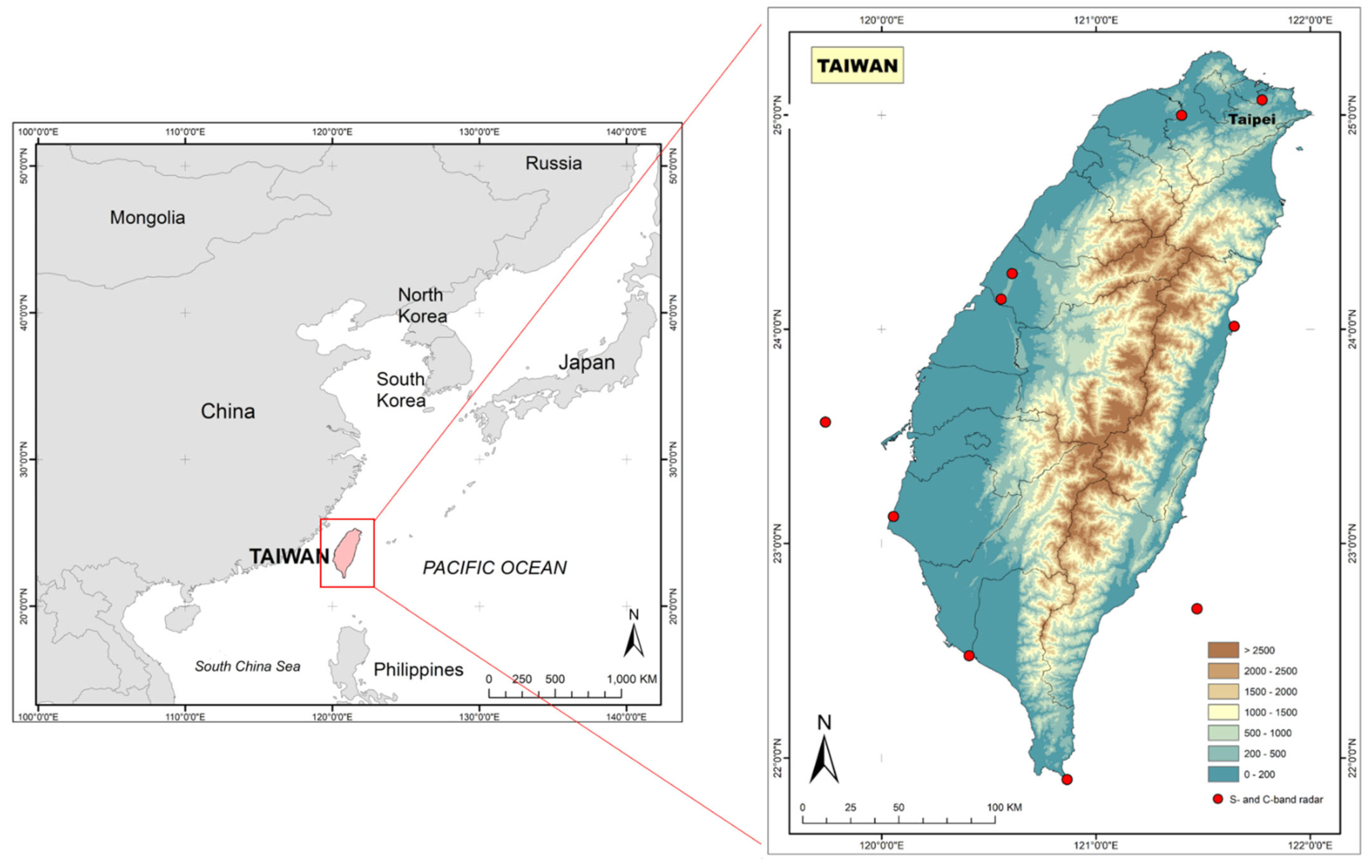
Taiwan, with a total area of 36,000 km2, is located in Southeast Asia’s Western Pacific (between Japan and the Philippines). Taiwan has a long and narrow shape, with the Central Mountain Range extending across the middle of the country. The mountainous area with elevations greater than 1000 m comprises 32% of the island, while hills and plateaus with elevations between 100 and 1000 m encompass 31% of the island, and the rest of the island is flat with elevations of less than 100 m (Figure 1).
Taiwan is situated in the East Asian monsoon zone, receiving 2500 mm of rainfall annually [30]. Taiwan is characterized by several adverse natural characteristics, including complicated terrain, short and swift rivers, and a position within the East Asian monsoon region and northwestern Pacific typhoon track. Additionally, during the Mei-Yu Rain Season in May and June, Taiwan is impacted by frontal systems, and the island is pounded by three to four typhoons each year [31]. This extreme meteorological phenomenon may occur during short periods of intense rainfall, resulting in slope collapse, landslides, and floods. On the other hand, during the dry season, from September to April, the southwest section of Taiwan often experiences several days without rainfall, which may result in droughts. A study by [11] found that extreme rainfall has been getting worse and more common for a long time, but the number of consecutive dry days has been going down in southwest Taiwan in recent years. Due to extreme weather and climate events in Taiwan, it is important to look at how the hydrological environment has changed.
Typhoons are the primary rainfall sources in Taiwan, followed by meiyu fronts, tropical low-pressure systems, and southwesterly flow occurrences [32]. These extreme meteorological occurrences can bring tremendous rainfall in a short period of time, resulting in flooding, landslides, slope collapse, and other problems. Between 1897 and 2018, the CWB reported that Taiwan issued an average of 6.8 typhoon warnings per year [11]. Taiwan receives an abundance of rainfall each year, ranging from 1600 to 3100 mm with an average of approximately 2500 mm. Additionally, extremely heavy rainfall with a maximum rate of more than 100 mm/h can occur during the summer season (May–October).
2.2. Data
The radar-derived rainfall data used in this study is QPESUMS (Quantitative Precipitation Estimation and Segregation Using Multiple Sensors). The QPESUMS system was created by Taiwan’s Central Weather Bureau (CWB) and the National Severe Storms Laboratory (NSSL) of the United States’ National Oceanic and Atmospheric Administration (NOAA). The QPESUMS system is primarily constructed of four weather Doppler radars that cover the entirety of Taiwan and the surrounding ocean. It measures base reflectivity with a high spatial resolution (0.0125°) and a temporal resolution of 10 min [33,34].
At the end of 2001, Taiwan’s Central Weather Bureau completed the Doppler radar observation network and implemented the QPESUMS system, which enhanced the monitoring, analysis, and early warning capability for violent or mutational weather. Quantitative radar rainfall estimation technology has advanced to the point that it can deliver more uniform and high-resolution spatial rainfall distribution information on a larger scale, hence establishing itself as the most effective method for increasing rainfall estimation accuracy [35].
In this study, the records of 22,787 grid pixels of QPESUMS are collected to cover the whole of Taiwan. The 24-h duration of the annual maximum series for the period 2006–2020 data was applied to conduct Regional Frequency Analysis (RFA) in Taiwan. The gridded rainfall dataset is the most recent data that has not been widely used in studies.
2.3. L-Moment approach
L-moments are linear combinations of order statistics that provide the expectation of particular linear combinations. The letter L denotes linear, indicating that L-moments are a linear function of the order statistics. L-moments are more robust to outliers in the data than ordinary moments. As a result, L-moments yield more reliable parameter estimations than conventional moments. L-moments was proposed as a modification of probability-weighted moments (PWMs) by [16,17]. For a distribution function, there are two cases of PWMs of the r-th order, and :
Ref. [17] defined L-moments as linear functions of PWMs for the ordered sample x1 ≤ x2 ≤ … ≤ xm of size m:
The L-moment ratios are expressed as follows:
where denotes the coefficient of L-variation (L-CV), is L-skewness (L-CS), and is L-kurtosis (L-CK).
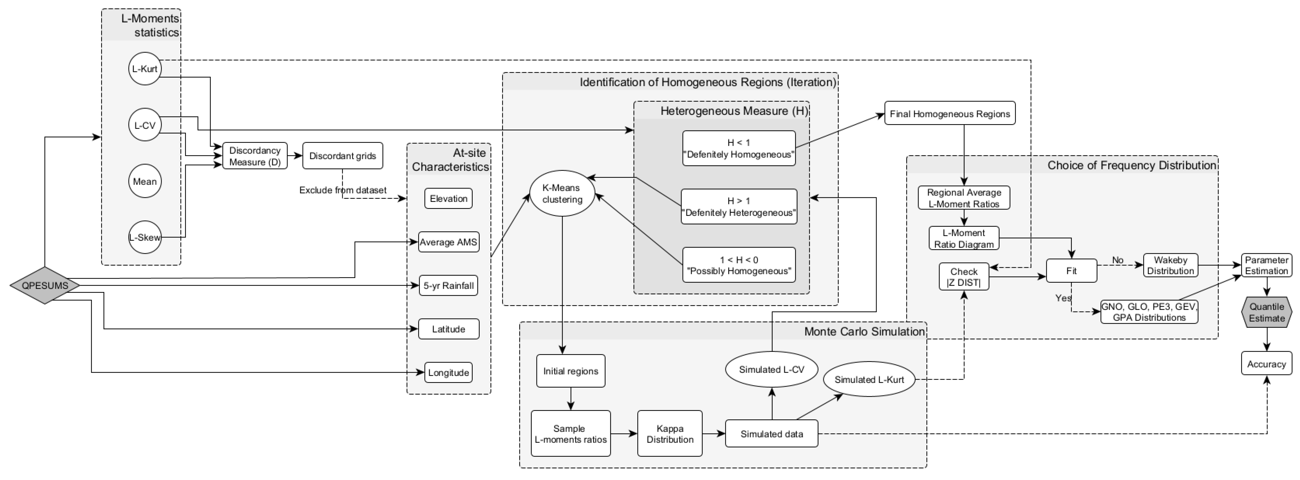
The L-moments and L-moments ratios are analogous to their ordinary moment counterparts, but they are more unbiased. Thus, these values can be used to describe the major characteristics of the distributions that are frequently utilized in extreme value analysis [36]. The L-moments procedures are available as an R package from CRAN (https://cran.r-project.org/package=lmomRFA, accessed on 12 July 2021) [37]. Figure 2 depicts a summary of the Regional Frequency Analysis procedures using L-Moments, and the section that follows explains the regionalization approaches in further depth.
2.4. Discordancy Measure
Hosking and Wallis (H) [15] discordancy measure is widely recommended for screening outliers’ sites in regional frequency analysis (RFA). Discordancy measures provide a discordancy metric for detecting anomalous sites in a region by utilizing the sample mean and sample covariance matrix of the site’s sample L-moment ratios including L-CV, L-skewness, and L-kurtosis. The performance of conventional and robust techniques for identifying discordant sites is evaluated using Monte Carlo simulations.
Assuming N stations are available in the area, the following three-dimensional vector of sample L–moment ratios of the yearly maximum daily rainfall sequence may be constructed and recorded:
The following are the discordant detection indicators:
A is a sample covariance matrix, N is the number of property vectors, is the vector containing L-moment ratios for the station i, and is the unweighted regional average value, is the measure of discordancy. Sites with > 3 should be considered discordant, according to [15]. To some extent, the criterion for discordance should increase as the number of sites in the region increases. This is due to the fact that sites with high values are more likely to be found in larger regions. In any case, regardless of the magnitude of these values, it is recommended to search the data for the sites with the highest values.
2.5. K-Means Clustering
Cluster analysis is a conventional approach of statistical multivariate analysis that can be used to break down huge and complicated data sets into a small number of data groups where members of a group have characteristics in common [38]. The supervised cluster algorithm approach, K-means, is applied to identify homogeneous regions across Taiwan. The K-mean clustering technique is chosen owing to its successful application in other rainfall regionalization studies [25,38,39]. In the K-means method, each cluster is represented by its centroid, which is the mean (weighted or unweighted average) of feature vectors within the cluster. This method is known for its efficiency in clustering large data sets with numerical attributes [40].
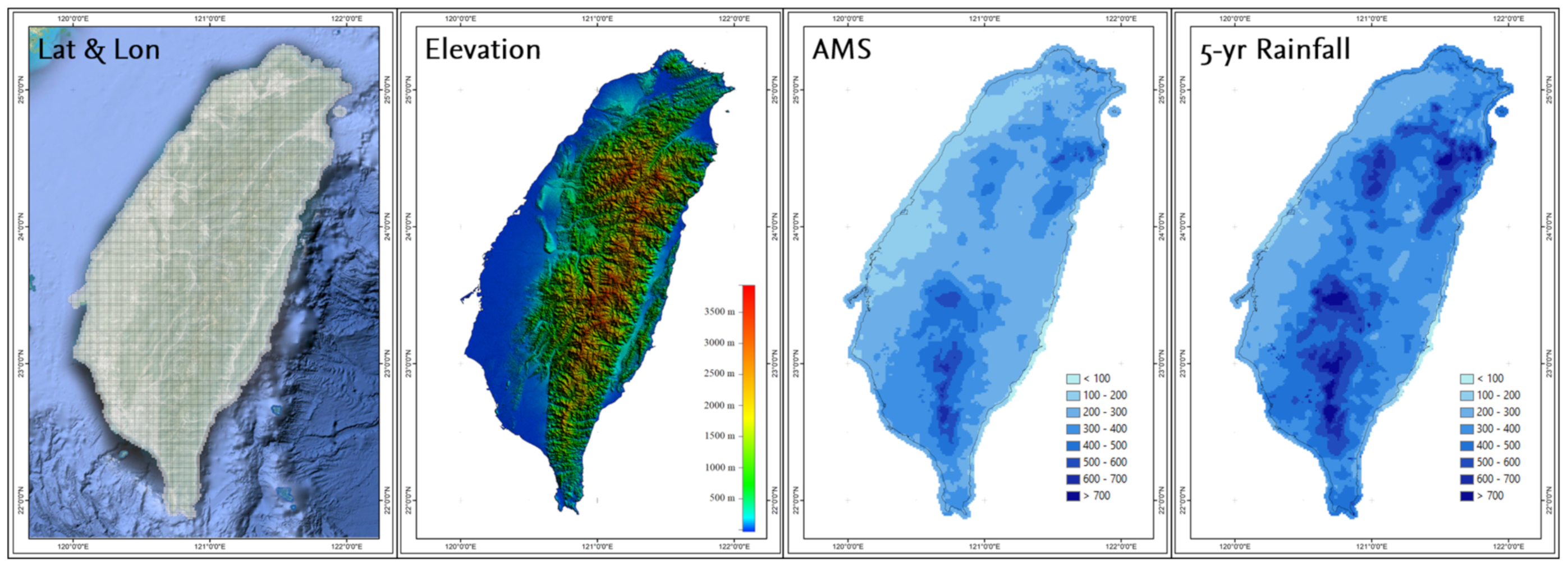
In this study, five dimensions/attributes known as site-characteristics are used in conjunction with the K-means algorithm to regionalize the rainfall extreme. The site-characteristics including latitude, longitude, elevation, the mean annual maximum series of each grid, and 5-year rainfall (Figure 3). Since variables with different units might impact the outcomes of the K-means clustering technique, the data should be standardized using suitable transformation functions before performing the algorithm [41]. As a result, the following variables/attributes of each site should be rescaled as follows:
where Y is the normalized value, and and are the minimum and maximum values for each variable in the data set (X), respectively. Cluster analysis does not always provide the desired results. Subjective enhancements are often required to promote physical continuity and reduce regional heterogeneity.
2.6. Heterogeneity Measure
The heterogeneity measure is used to determine if proposed regions generated by cluster analysis of site attributes could be considered as homogenous. Hosking and Wallis’s heterogeneity measure (H) is often used in regional frequency analysis to assess regional homogeneity. This statistic is calculated using dispersion measures, which are defined as the total of the errors between the at-site sample L-moment ratios and the regional average L-moment ratios. Using Monte Carlo simulation, a measure of heterogeneity generates several simulated regions from a flexible probability distribution and compares observed and generated data [42]. Ref. [15] estimates heterogeneity by parameterizing the more flexible four-parameter Kappa distribution using data from the candidate region, from which simulated regions are produced using Monte Carlo sampling. A statistic V can be computed for the actual region and all simulated regions as the total of the squared deviations from the mean across all sites for a given L-moment ratios. To estimate H, the mean and standard deviation of V over all simulated regions are calculated and compared to V for the actual data. The heterogeneity measure is calculated as follows:
where is the standard deviation of at-site sample L-CV. and mean and the standard deviation of the simulated values of V, respectively. is the regional L-CV of either actual data or simulated data.
Ref. [15] classify an area as acceptably homogeneous when H < 1, possibly heterogeneous when 1 ≤ H < 2 and definitely heterogeneous when H ≥ 2. If the value of H1 did not fulfill the criterion, the site inside the region needed to be modified to meet the requirements for becoming an approved homogenous region. Ref. [15] then proposed several region changes, including the following: (1) relocating a site or a few sites within a region; (2) subdividing the region; (3) merging two or more regions and redefining groups; (4) breaking up the region by reassigning its sites to other regions; and (5) removing a site or sites from the data.
2.7. Selection of Candidate Distributions
Ref. [15] suggested two methods for determining the best-fitting distribution: The L-Moment ratios diagram and the Z-test. The L-moment ratio diagram is a visualization of the distribution function’s calculated L-skewness and observed L-kurtosis values. The curves represent potential links between the proposed distribution’s L-Cs and L-Ck [43]. L-moment ratio diagrams have been proposed as a handy tool for differentiating between alternative distributions that might be used to represent regional data. The sample average and a line of best-fit through the sample L-moment ratios are two graphical tools used to aid in distribution selection. The closeness of the sample average or the record length weighted average to the theoretical curve or point in L-skewness and L-kurtosis space of a given candidate distribution has been regarded as an indicator of the distribution’s suitability to represent the regional data.
The Z-test is a statistic that reflects how well the theoretical L-kurtosis of the fitted distribution matches the regional average L-kurtosis of the observed data. The quality of fit is determined for each of the candidate distributions by:
where denotes the candidate distribution and denotes the fitted (candidate) distribution’s L-kurtosis obtained via simulation for the purpose of estimating the fitted distribution as follows:
where are the coefficients described in [15], denotes the bias of the regional average sample L-kurtosis () determined using simulation approach with denoting the sample L-kurtosis of the mth simulation:
and σ4 is the standard deviation of regional average sample L-kurtosis estimated as
A fit is regarded satisfactory if |ZDIST| is sufficiently close to zero, with |ZDIST| being less than or equal to 1.64. If there are more than one acceptable distribution, the one with the lowest |ZDIST| is considered to be the best distribution.
Generalized Normal (GNO), Pearson Type III (PE3), Generalized Extreme Value (GEV), Generalized Logistic (GLO), and Generalized Pareto (GPA) Distributions are the candidate distributions considered in this study. If the three-parameter frequency distributions do not match the rainfall data well, we may try fitting using a five-parameter Wakeby distribution. Wakeby distributions have more parameters than other system distributions, allowing for a greater variety of shapes and a relatively good fit to any sample [44].
2.8. Estimation of Rainfall Quantiles
The index-flood approach is used in regional frequency analysis to determine quantiles for each station’s distinct return periods. The index flood method assumes that rainfall from multiple locations within a region is normalized by their mean annual rainfall from a single distribution. The index flood technique works on the premise of defining rainfall at each site as two components, one representing the rainfall specific to the location and the other reflecting the rainfall features common to the homogenous region. Equations (16) and (17) determine the parameters of the fitted frequency distribution from the regional average L-moment ratios, which are weighted proportionately to the site’s record length, respectively.
Finally, the quantile estimates at site i are obtained from the index flood and regional quantile function q(F)F given by:
2.9. Accuracy Assessment
Uncertainty is a necessary component of every statistical estimate. The related uncertainty of an estimated quantile indicates how dependable the value is for confident usage. Ref. [15] suggested an evaluation approach that includes utilizing a Monte Carlo simulation to generate regional average L-moments. Quantile estimations for different return durations are computed in the simulation. The computed quantiles for non-exceedance probability F is at the mth repetition. The relative error of the estimate at station i for non-exceedance probability F is . This amount can be averaged across all M repeats to approximate the estimators’ relative RMSE. The relative RMSE for a large M is approximated by:
The regional average relative RMSE of quantile estimates provides an overview of the accuracy of quantile estimations across all grids in the region:
Analogous values can be calculated for growth curve estimations, but with and substituted by and , respectively. The 90% error bounds for are:
where and are the values where approximately 90% of simulated values to true value ratio, i.e., lies. We simply multiply the relative error measurements by the calculated quantiles to obtain the absolute error measures.
2.10. Regional and Grid-Based Estimates for Watershed Scale
Extreme rainfall patterns are commonly characterized using at-site and regional frequency analysis. While at-site frequency analysis uses only records from the target location (grid/station) to estimate the quantiles, regional frequency analysis makes use of data from stations with comparable rainfall patterns to produce more precise estimates of extreme rainfall intensities. In this part, we analyzed the difference and similarity between regional and grid-based (at-site) estimates at several return periods at one particular watershed. In this study, we select the Touqian watershed. The reason for this comparison is that regional estimates, when applied at the watershed-scale, sometimes have high uncertainties and cannot be applied, especially in regions that have complex topography and rainfall patterns. This is due to the different approaches where at-site analysis considers at-site characteristics and at-site statistics only for the entire watershed area, while regional analysis, when applied to watersheds, also considers at-site characteristics and at-site statistics for all grids/stations in each homogeneous region where part of the area is in the watershed.
To analyze the differences between the two approaches, we use a spatial approach with visual and statistical comparisons at 50-year return period. Furthermore, the similarity analysis uses an image matching approach. Normalized Cross-Correlation (NCC) and Jaccard Similarity Index (JSI) were used to measure the degree of similarity between the two approaches. NCC is one of the most effective and commonly used similarity metrics in matching tasks. The Normalized Cross-Correlation (NCC) of two time series can be defined as
where n is sample size, xi and yi are the individual grids indexed with i, X and Y are the regional and at-site (grid-based) datasets.
Jaccard Similarity Index (JSI) is a statistical value used to compare the similarity and diversity between two different sample sets. Jaccard similarity is defined as the magnitude of the intersection of the two sets divided by the magnitude of the union of the two sets (Equation (21)). The larger the value, the more similar condition for the two groups [45].
In this study we used weighted Jaccard Similarity Index. In this measure, the high similarity between a pair of points indicates that the points have high resemblance, meanwhile low similarity indicates that the points are distant. Weighted Jaccard Similarity computed between two vectors or data points x and y where each of vectors has a length of n is the summation of the minimum of two vectors in each dimension divided by the summation of the maximum of those two vectors in each dimension. The calculation of weighted JSI can be seen in the following equation.
Practically, the numerator is the intersection of two vectors and denominator is the union of two vectors. The Jaccard Similarity Index between two vectors is 1 when those two vectors are the same and is 0 when those two vectors do not have anything in common (that is the numerator is zero).
3. Results & Discussion
3.1. Screening the Data
Validating the acceptability of the data for the analysis by screening for unusual data items is a crucial part of any statistical data analysis. The discordancy measure, Di = D(ui), should tell us how distant ui is from the center of the area in respect to its size. Large Di values suggest that the ith site should be examined further for the potential of data errors, or that the prospect of relocating the site should be considered.
When assessing the discordancy test results generated for the stations, grids with a D value of 3 and higher are recommended to be eliminated from future regional studies since they could not pass the discordancy test when the cluster size is more than 15. To some degree, the discordancy criteria should be a function of the number of sites in the area. This is because sites with high Di values are more likely to be found in large regions. In any case, regardless of the size of these values, it is recommended to study the data for the locations with the highest Di values [15].
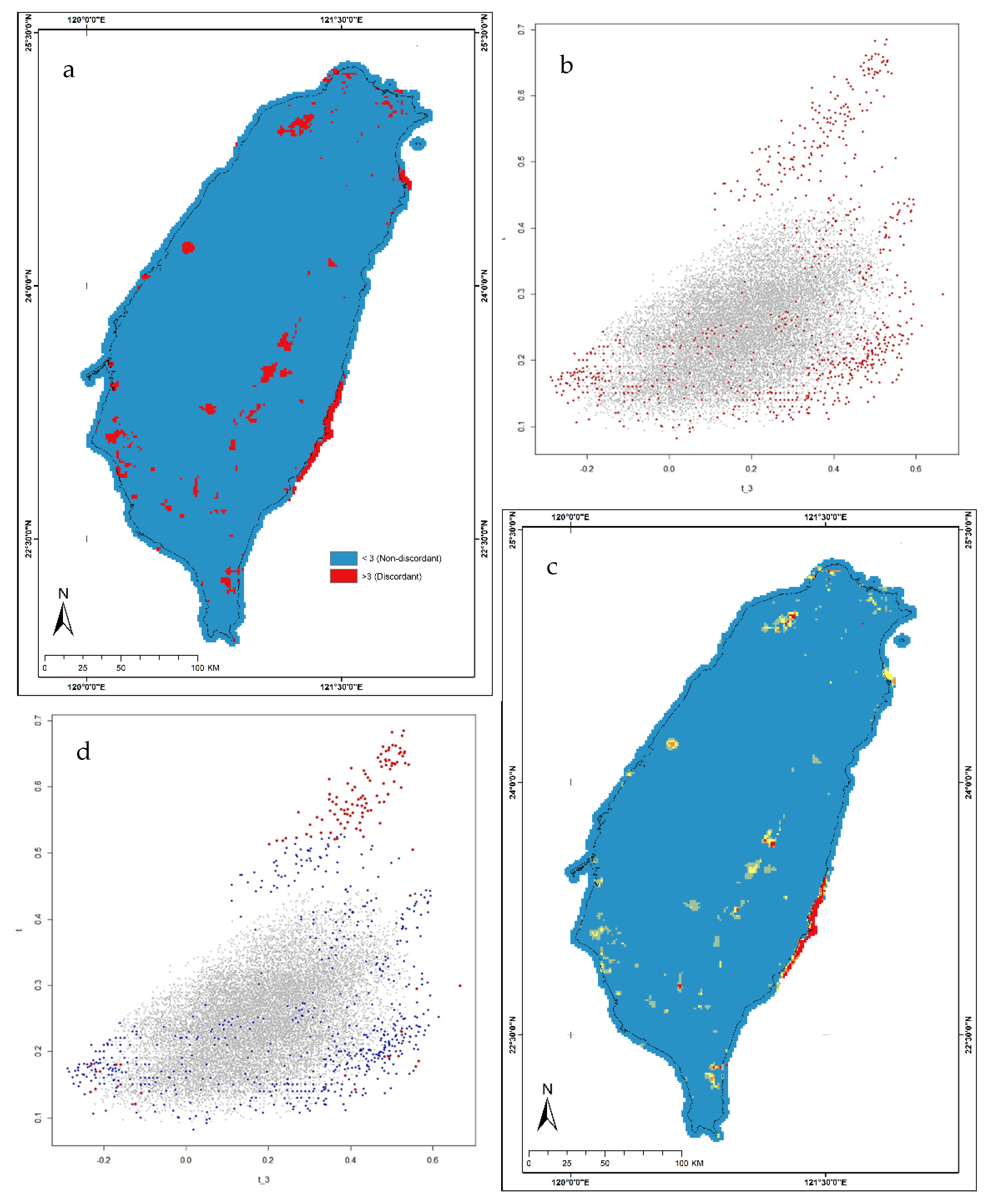
Based on the above theories, we conducted two discordance test approaches, first by using a critical Di of more than 3 and the second using a critical value of >6. Figure 4a,b show the discordant spatial grid distribution (Di > 3) and a graph of the relationship between L-skewness and L-CV. A total number of 801 of 22,787 grids is categorized as discordant (3.52% of total grids). The spatial distribution of discordant grids is almost evenly distributed throughout the region, but a continuous significant discordant grid is seen in the southeastern area.
After further testing, we found that, to some extent, the grid with Di values > 3 (discordant) did not affect the homogeneity of the region after clustering and heterogeneity tests. therefore, we continued the second analysis by increasing the critical Di limit by >6. Based on this critical value, 171 of 22,787 grids are categorized as discordant (0.75%) (see Figure 4c,d). Grids with discordant value greater than 6 greatly affects the homogeneity of the region. The region that was originally homogeneous shifted to heterogeneous, especially in the southeastern region.
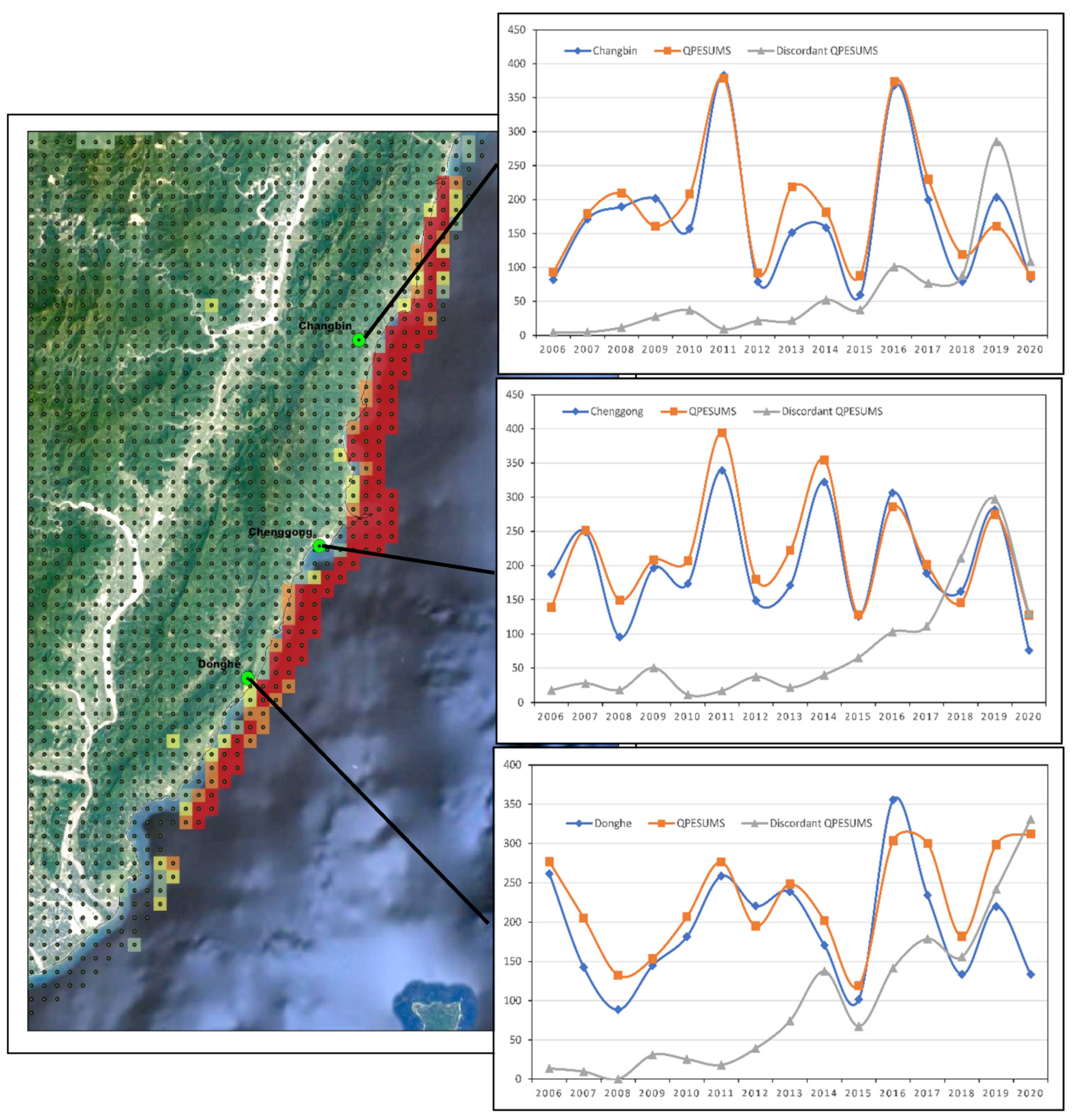
After conducting further investigations in the southeast (discordant grid > 6), by comparing the radar estimation value (QPESUMS) with the three closest rainfall stations, we found that the QPESUMS rainfall values were extremely underestimated compared to the rain gauge values from 2006–2015 (Figure 5) but after 2016, the value tends to be similar. According to [46], due to the island’s two major mountain ranges (the Snow Mountain Range (SMR) and the Central Mountain Range (CMR)) and the significant blockages caused, the S-band radar network’s vertical coverage in the inner island was severely limited. For large swaths of the SMR and CMR, the lowest 1 km of the atmosphere is not covered by radar. These vertical coverage gaps adversely impacted the quality of precipitation forcing used in hydrological forecasting, and additional radars are required to address these gaps. Since 2016, four additional C-pol radars have been placed island-wide to enhance radar coverage at low altitudes. As a result, the C-pol radars considerably improved low-level coverage, particularly along the east coast and throughout a major portion of northern and southern Taiwan. Based on that consideration, the discordant grids with DI > 6 were excluded for further analysis.
3.2. Identification of Homogeneous Regions
Determining the number of subregions is critical in the work of L-moment because an insufficient number of subregions will result in an inappropriate division pattern that may not meet the RFA’s homogeneity requirement [47]. The number of subregions in this research was decided by first establishing an initial number based on regional geographical factors and then shifting the number back and forth until all split subregions passed the homogeneity test. This determination employs the K-means clustering method and subjective adjustment. in K-means clustering method, five factors called site-characteristics including latitude, longitude, elevation, mean annual maxima, and 5-year rainfall are employed to subdivide the whole Taiwan island into subregions, while the subjective adjustment is used to ensure that all regions are homogeneous. Since the QPESUMS data has a very large grid (22,787 grids), the use of the K-means clustering method alone to regionalize the frequency of analysis will be very difficult; therefore, it needs to be refined by subjective adjustment [38]. The region should be sufficiently large to have a large sample size (many extremes) and small enough to neglect extreme statistic variability [29].
For each region, discordancy and heterogeneity measures (Di and H1) defined in Equations (5) and (9) were calculated to see if they are spatially continuous and physically reasonable. When the estimated heterogeneity measure (H1) surpasses the critical value, which indicates “potentially” and “definitely” heterogeneous, K-means then will be used to regroup the grids in the region into smaller regions. This process was repeated until no further separation of heterogeneous regions was possible. Occasionally, the discordance measure suggested that several surrounding grids within a region are discordant with the remainder of the region. In this case, the homogenous regions were manually refined by using subjective adjustments as described in the methodology section. Examining the discordant grids showed several natural and physically defensible modifications to the clusters, leading to more homogeneous clusters after accounting for the topographical and geographic patterns of the average annual maximum series.
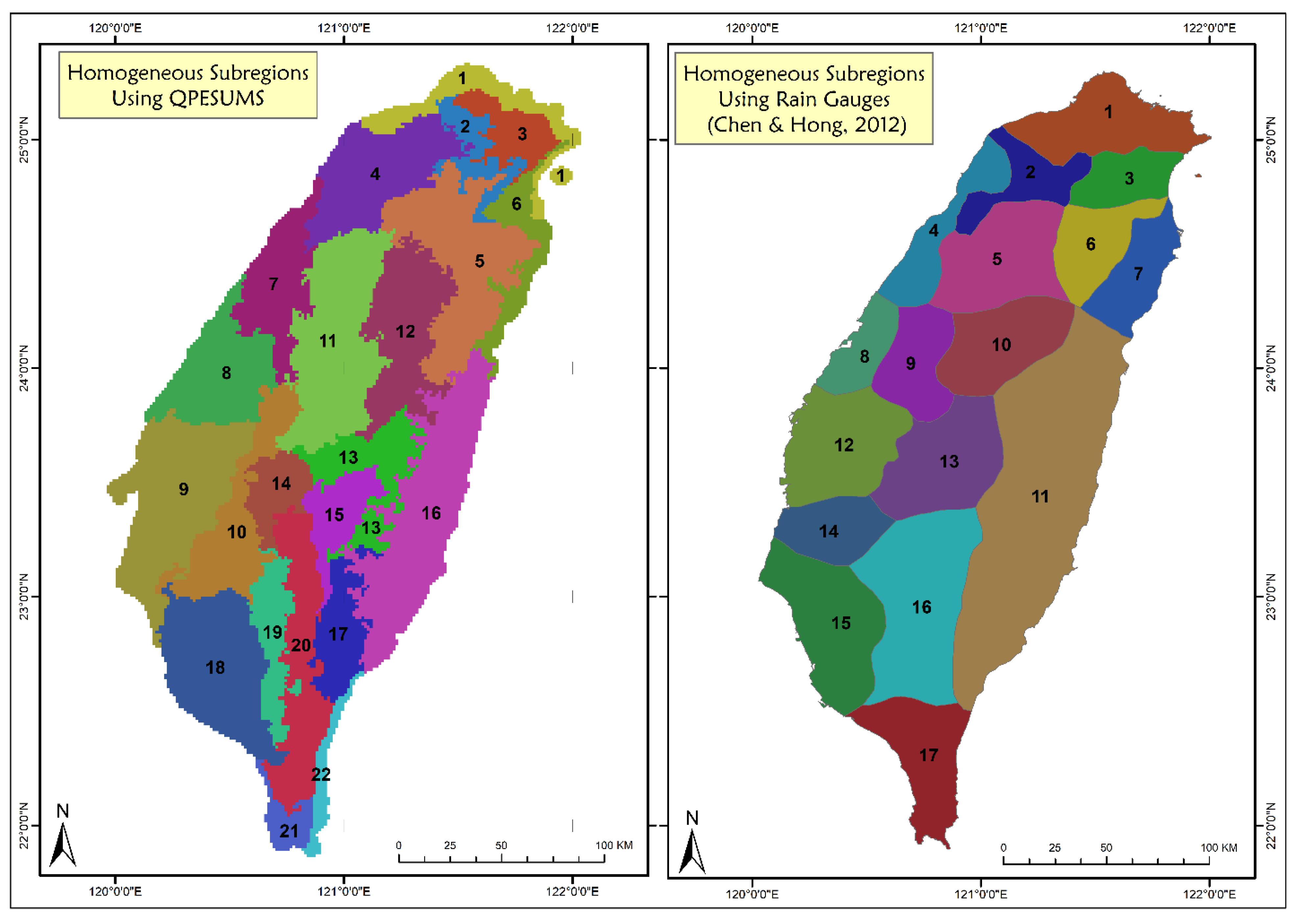
A total of 15 initial clusters/sub-regions were determined by using the K-means clustering method. Furthermore, a total of 22 sub-regions are discovered to apply to the study area after subjective adjustments. The 22 subregions were defined as geographical areas with similar topography and climatological characteristics that experienced similar meteorological conditions during storm events. We depict the boundaries of the 22 subregions in Figure 6. This regional classification is similar to the findings of [48] which divides Taiwan into 17 homogeneous sub-regions. They divided sub-regions using the principal component analysis method, self-organizing maps, and L-moment using 127 rain gauges data. Limited spatial density using uneven rain gauges makes interpolation difficult and makes it difficult to produce maps with clear homogeneous boundaries. Ref. [49] in their research that compares mapping approaches of design annual maximum daily precipitation also concludes that one of the problems or difficulties of the regional approach is the discontinuity of boundaries between sub-regions. They suggest that in the future, the use of radar-based rainfall could be a solution. We utilized 22,787 radar-rainfall grids with a very high spatial resolution for our study. In contrast, two earlier studies from [38,48]) relied on rainfall data from rain gauges that were not evenly distributed and totaled 154 and 127 rain gauges, respectively. We also employ a distinct clustering algorithm, K-means, as opposed to their SOM. Regardless of type, clustering algorithms are also extremely sensitive to differences in the number and scale of parameters. Here, the gridded data from QPESUMS play a crucial role in identifying the characteristics and number of homogenous regions. With thousands of grids coupled with other physical parameters such as latitude, longitude, elevation, the average of annual maximum series, and 5 years of rainfall, it is possible to distinguish homogeneous regions, particularly in the middle, which is a mountainous region where the number of rain gauges is still limited. We have discussed this affirmation in the result section. Our findings further confirm that, using QPESUMS which is based on high resolution radar-based rainfall, we can produce homogeneous regions that are not only similar, but also more detailed with clear boundaries between regions, especially in the center/mountain range area where the number of rain stations is still very limited. In other words, we have better results in terms of detail.
Geographically, the 22 sub-regions are divided into five regions: the northern region (sub-regions 1–6), the western region (sub-regions 7–10), the center region (sub-regions 11–15), the eastern region (sub-regions 16 and 17), and the southern region (sub-region 18–22). Table 1 shows the total number of grids in each sub-region, as well as their L-moment ratio. According to Table 1, the biggest sub-region is sub-region 16, which is located in the eastern region and has a total grid of 2231 grids, whilst the smallest sub-region is sub-region 22, which is located in the southern region and has a total grid of 248 grids. In contrast, the northern and southern areas of Taiwan have complicated distribution patterns of homogenous sub-regions. The results of heterogeneity tests for annual rainfall data are also summarized in Table 1. It can be seen that all regions are “acceptably homogeneous”, with H < 1. These results demonstrate that the 22 regions are sufficiently homogeneous.
3.3. Selection of Distribution Models
The determination of appropriate regional frequency distributions is also important in the RFA. An inappropriate selection of distributions may result in a large overestimation or underestimation of extreme rainfall. Rainfall maxima are often positively skewed, having a comparatively longer right tail. Three-parameter frequency distributions are much more flexible than two-parameter distributions, which may enhance fit in the right upper tail region. Three-parameter frequency distributions are primarily very popular, and they are frequently used in the context of a regional frequency analysis (RFA) method.
The L-moment ratio diagram is widely used as the first visual assessment tool for selecting a regional frequency distribution from sample data collected in a particular location. The sample L-moment ratios, regional average L-moment ratios, and theoretical L-moment ratio curves of candidate distributions are displayed in an L-skewness and L-kurtosis space. The theoretical plotting positions of the candidate distributions are given using polynomial approximations.
L-moment ratio diagrams have been used to show averages of L-skewness and L-kurtosis in 22 homogeneous regions. Then, theoretical curves for different distributions have been shown, as well (Figure S1). As long as the point that is the regional average is close to the curve that corresponds to a certain distribution, this distribution will be a good choice for the parent distribution in the region. As shown in the L-moment ratio diagrams (Figure S1), in 11 of Taiwan’s 22 subregions, the regional average L-moment ratios do not approach or are exactly on the theoretical curves of five candidate distributions. As a result, [15] suggest that the Wakeby (WAK) robust distribution is the most appropriate.
More precisely, the z value indicates the degree to which the regional mean distribution fits the five alternative distributions the best. According to the z value in Table 2, the best fit parent distribution of half of six subregions in the northern region, specifically subregions 1, 3, and 6, is dominated by the GEV distribution. Only subregion 8 in the western region has a Z value that does not fit any of the five possible distributions. While the Wakeby (WAK) distribution best fits all subregions in the east and center regions. Finally, Generalized Pareto (GPA) best fits as a parent distribution in the southern region. Moreover, Table 2 also shows the distribution parameters of the best-fit parent distribution for each subregion. A way to figure out how well a distribution fits is to look at how far samples points are from the curve for that distribution. Additionally, the optimal distribution determined at this stage will be used to calculate the regional growth curve for each homogenous region.
In addition to using the five three-parameter distributions and the Wakeby five-parameter distribution as parent distributions for each homogeneous region, we also recommend using a four-parameter distribution such as the TCEV (Two-Component Extreme Value) distribution [50,51], which is ideally suited for a regionalization approach. The estimation of this distribution from an at-site data series is suitable if the sample size N is adequate (at least 90–100 data) [52].
3.4. Estimation of Regional Quantiles
Following successful selection of the most appropriate regional frequency distribution, the regional quantiles for various return periods are estimated using the parameter estimates for the distributions in Table 2. The index-flood method is used to estimate the quantile estimations at varied non-exceedance probabilities and recurrence intervals for 22 sub-regions in Taiwan in the current study. The index flood technique, which normalizes data at each site by dividing by the sample mean or median, is one of the most often used ways for regional frequency analysis.
Table S1 shows the desired rainfall quantile estimates with different return periods for each homogeneous region. It can be seen that the selected regional distributions for each sub-region predict quantiles that are very comparable. Additionally, Table S1 demonstrates that the variation in the range of quantile estimations grew from 0.80–0.99 in a 2-year period to 1.71–3.35 in a 100-year return period. This result explains that the variation in quantile estimate would increase as the return duration increases.
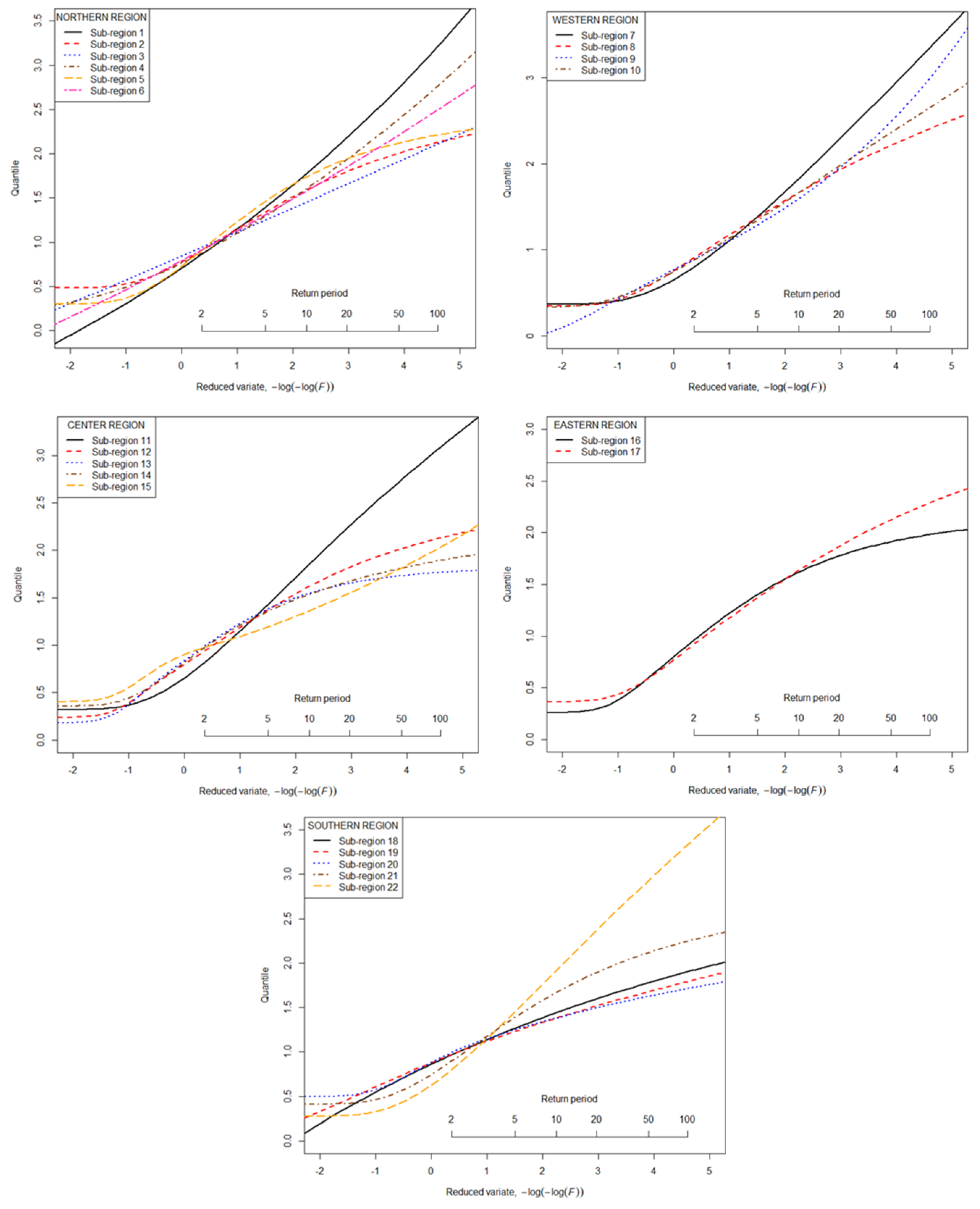
The regional growth curve, which was based on the regional distribution, was plotted for a set of return periods (Figure 7). This growth curve depicts the variation of the regional quantile (growth factor) q(F) versus the not-exceeded probability F or the return period T (T = 1/(1 − F)). According to the variation of the growth curves for 22 homogeneous regions in Figure 6, sub-regions 1, 7, 11, and 22 have higher regional growth curves in the higher return period than other sub-regions, whereas sub-regions 13, 19, and 20 have the lowest. There are no results that show which distribution has a higher or lower growth factor. The level of growth factor, on the other hand, is influenced by site characteristics, particularly the annual maximum series and elevation. Sub-regions 13, 19, and 20 are sub-regions with high annual maximum series and a higher average elevation.
3.5. Accuracy Result
Although the estimates obtained through regional frequency analysis are reliable, we still require specific measures to assess the accuracy of these estimates. Table S2 displays the relative regional RMSE values and 90% error bounds. Table S2 shows that the RMSE and error bounds increased in line with the increase in the return period. It is clear that the uncertainty of regional quantiles grows with the return period. In the upper tail, high RMSE values and error bounds are observed, indicating the unreliability of quantities with return period T > 100 years.
Table S2 further demonstrates that the root mean square errors of the predicted regional growth curve and the quantiles for 22 homogenous regions range from 0.002 for a 2-year return period (sub-region 18) to 0.158 for a 100-year return period (sub-region 18), respectively (sub-region 9). The RMSE values indicate that the estimate of extreme rainfall is reliable up to a return period of 100 years. It will be necessary to collect more historical data for estimates of longer return periods in order to improve the reliability of the quantile estimation. Additionally, Table S2 includes the 90 percent error boundaries, demonstrating that the quantile estimations are sufficiently accurate when return periods are shorter than 100 years. This result is also consistent with [53]’s regional frequency analysis of precipitation extremes in China’s Hanjiang River Basin. They discovered that when the return time exceeds 1000 years, the RMSE values are relatively large, implying that quantile estimations are sufficiently reliable when the return period is less than 100 years, and then become unreliable as the return period increases.
3.6. Spatial Mapping of Extreme Rainfall
The occurrence of extreme rainfall is a primary natural hazard in many regions of the world, and the development of maps depicting this hazard is of great theoretical and practical importance. In order to map the spatial distribution of extreme precipitation, it is necessary to convert the discrete data collected at various climatic stations in a region into a spatially continuous variable [54]. Frequently, interpolation techniques such as IDW and Kriging are used to map extreme precipitation. The issue is that the quality of a spatial interpolation depends heavily on the number and distribution of points [55]. Regional frequency analysis utilizing gridded QPESUMS data has benefits including uniform distribution and high spatial resolution. Using sample average annual maximum series as the at-site function and regional quantile as the regional function, we can map extreme rainfall for each return period with a resolution of 0.0125 degrees, as shown in Figure 8. In this analysis, the maps were generated using GIS technique. Extreme rainfall for a 24-h duration and return period (2, 5, 10, 20, 50, and 100-year) were created by importing all the point values and convert into grid/raster values. The rainfall extreme values are obtained from the index-flood approach, which multiplies the regional growth factor of different return periods by the average annual maximum series of 22,787 QPESUMS grids as index-flood.
Figure 8 illustrates the spatial patterns of extreme rainfall for different return periods. There are two significant regions with the highest rainfall extremes especially for a 100-year return period with extreme value more than 1200 mm/day. One is the eastern part of northern region (mainly sub-region 5), which is in Yilan County, and the other is in the southern region (sub-region 10, 14, 15, 19, and 20), which is part of Tainan City, Chiayi County, Kaohsiung City, and Pingtung County. These two places are frequently struck by typhoons. The closure of the central mountain range has a profound effect on the spatial distribution, frequency, and intensity of typhoon extreme rainfall. [56] investigated, utilizing CWB hourly precipitation data from stations, and discovered that the typhoon extreme rainfall pattern is phase locked to the central mountain range (CMR), and that topographic forcing plays a critical role in typhoon extreme rainfall.
3.7. Regional and Grid-Based Estimates for Watershed Scale
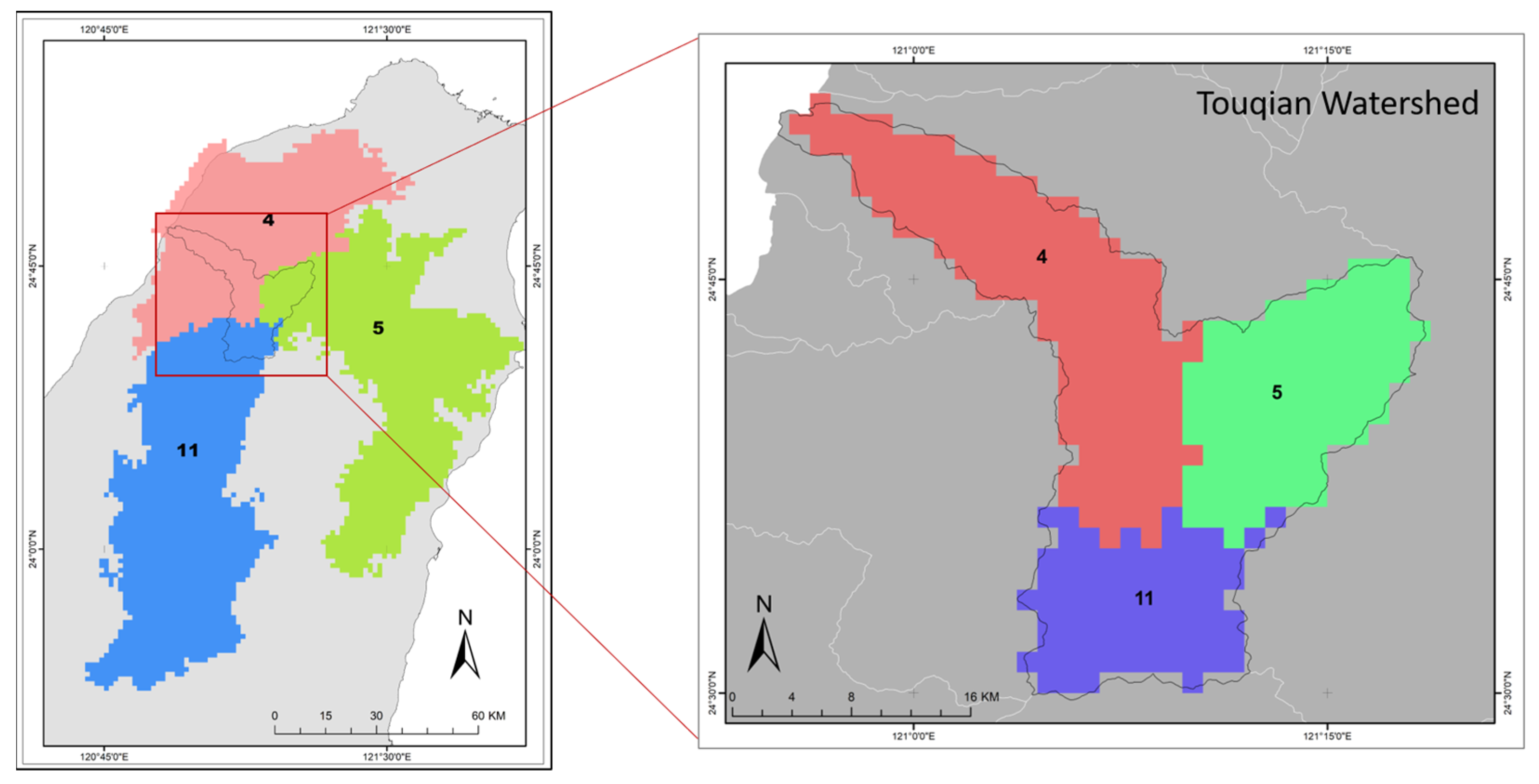
Extreme rainfall patterns are commonly characterized using at-site and regional frequency analysis. In the previous part, it has been proven that regional frequency analysis has been able to estimate and display extreme rain for the entire Taiwan area. However, in such a case, a comparison with at-site analysis is advised, particularly in smaller scale regions. In this part, we were analyzed the difference and similarity between regional and grid-based (at-site) estimate at several return periods at Touqian Watershed (Figure 9).
As seen in Figure 9, there are three homogeneous sub-regions within the Touqian watershed, including sub-region 4, 5, and 11, with a total of 322 grids or 566 km2 within drainage area and a total of 5103 grids for the three homogeneous subregions. More specifically, of the 322 grids within the Touqian watershed, 145 grids are located in subregion 4 (10.67 % of total SR-4 grids), 101 grids are located in subregion 5 (5.59 % of total SR-5 grids), and 76 grids are located in subregion 11 (3.92 % of total of total SR-11 grids).
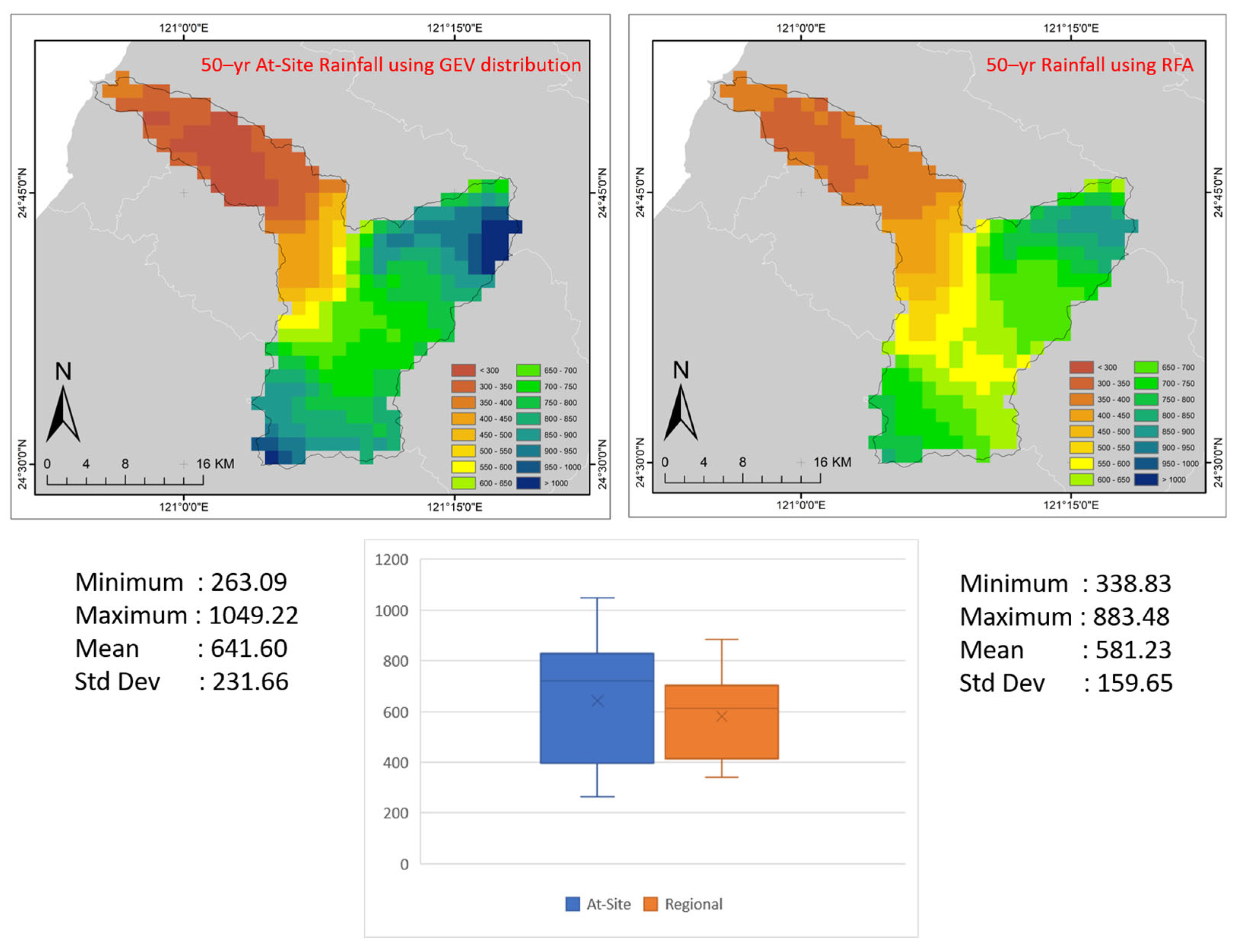
Spatial distribution of extreme rainfall and statistics for a 50-year return period at-site frequency analysis using the GEV distribution and for a 50-year return period using regional frequency analysis is depicted in Figure 10. It is not clear which frequency distribution is best for estimating extreme hydrological events, but the GEV distribution is theoretically a good fit for the annual maximum series of extreme hydrological events. As can be observed from the at-site analysis, rainfall varies from 263.09 to 1049.22 mm/day, with an average of 641.6 mm/day. Meanwhile, regional analysis indicates a narrower rainfall range, with a minimum of 338.83 mm/day and a maximum of 883.48 mm/day, with a lower average of 581.23 mm/day. Spatially, extreme rainfall is comparatively larger when at-site analysis is used, particularly in the upper part of the Touqian watershed, which is part of subregions 5 and 11. This result indicates that regional frequency analysis may yield more precise estimates of rainfall quantiles than at-site analysis not only for a larger area but also for a smaller-scale area.
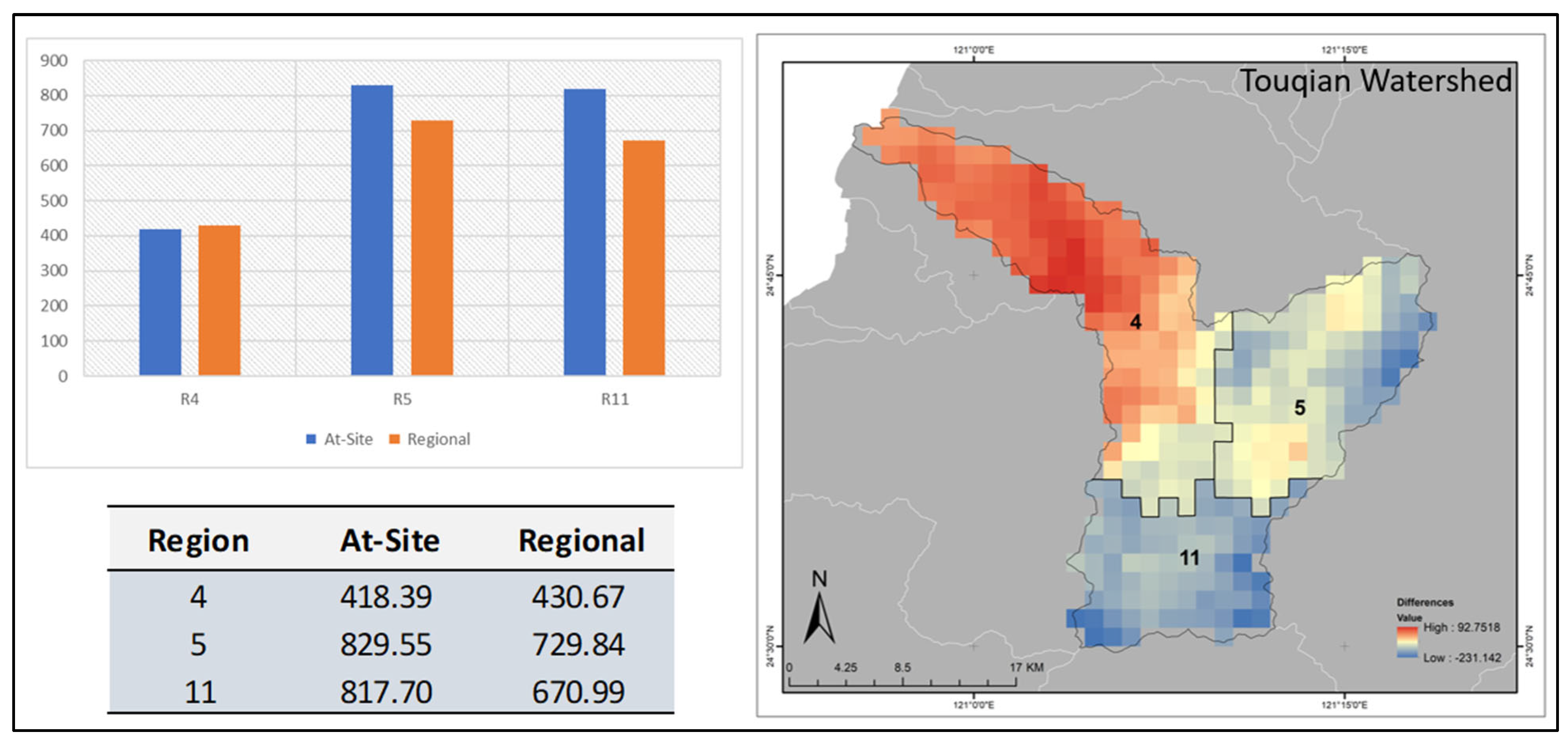
Figure 11 illustrates the extent to which the two analyses’ estimates of extreme rainfall differ. As can be observed, the difference in the value of extreme rainfall estimates is not significant in subregion 4; however, the difference is rather significant in subregions 5 and 11. The average extreme rainfall for at-site and regional analyses in subregion 5 was 829.55 mm/day and 729.84 mm/day, respectively, whereas in subregion 11, it was 817.7 mm/day and 670.99 mm/day.
Figure 12 and Table 3 depict similarity measures between the grid-based and regional approaches at Touqian Watershed and for the whole Taiwan as a reference for different return periods. Based on that figure and table, the NCC values for Touqian are around 0.9, which means there was a higher correlation between grid-based and regional. The same was true for the correlation for the whole of Taiwan. The difference is that for the Touqian watershed (small-scale), the correlation tends to be stable while for the Taiwan (big-scale), the correlation tends to decrease as the return period increases, although it was not very significant (from 0.97 at 2-year to 0.84 at 1000-year). Likewise, the JSI value, which has a range from 0.79 to 0.93, which explains that there was a high similarity between grid-based and regional approaches for both small-scale and big-scale. Both scales also show a decrease in the level of similarity along with the increase in the rainfall return period. Interestingly, the similarity value for Touqian is lower than for Taiwan at a higher return period. This result is in line with the accuracy results using Monte Carlo, which demonstrates increasing uncertainty in higher return periods. [57] also suggest, for higher return periods, the estimation of extreme rainfall should be treated with caution and longer rainfall data is required. By using grid-based as the basis for assessing regional frequency analysis, these results show that the regional approach in determining extreme rainfall is very suitable for large-scale applications and even better for smaller scales such as watershed areas.
3.8. Small-Scale Spatial Investigation
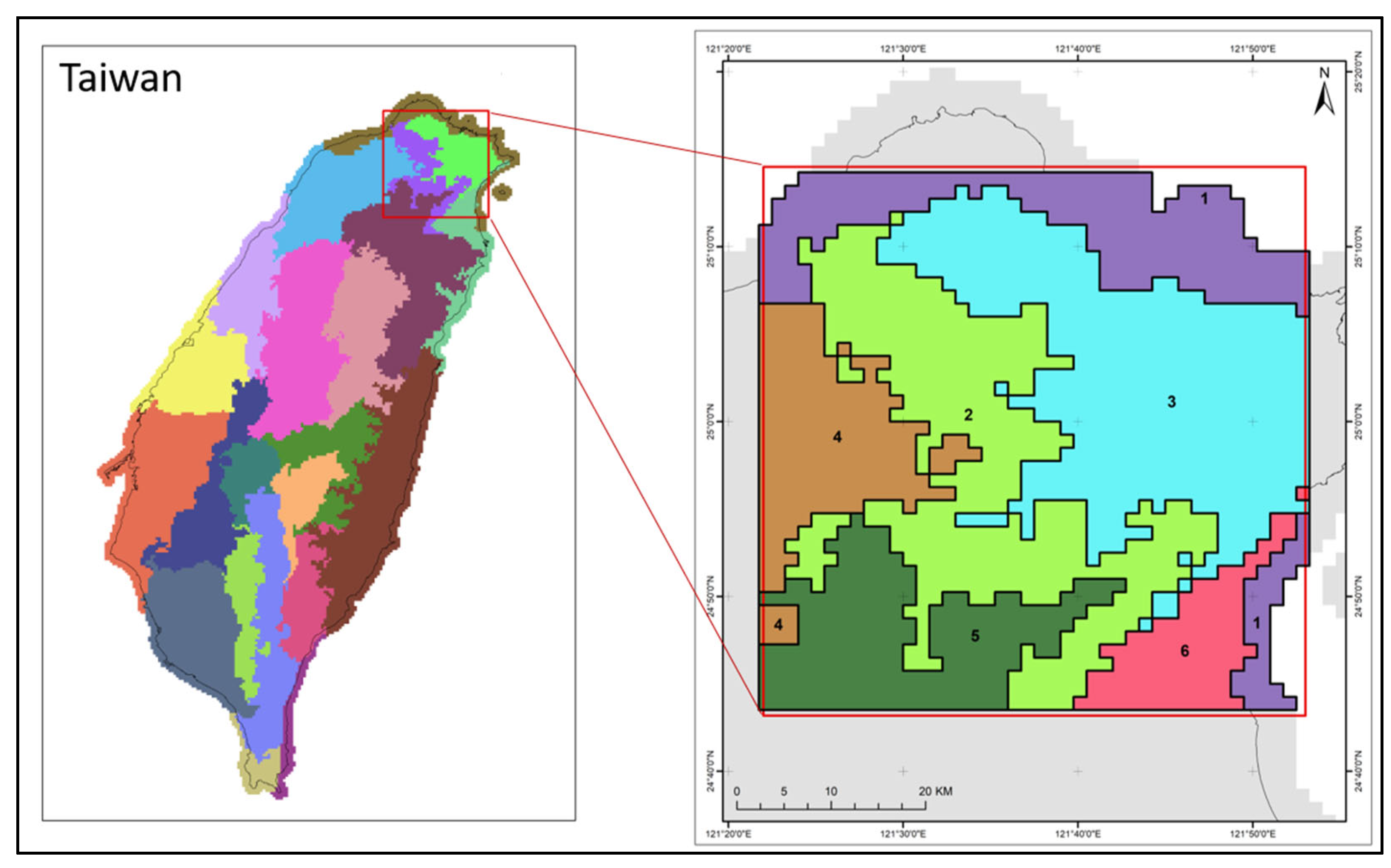
A spatial investigation in a more specific area is carried out to determine the accuracy of regional frequency analysis. According to [58], certain inaccuracies are to be expected when applying the approach to different geographical locations with reduced spatial variance. The spatial investigation in this study was carried out by establishing a region of interest in the northern part of Taiwan (Figure 13). The northern part of Taiwan was chosen as the region of interest because it has several small homogeneous subregions and a more dynamic rainfall pattern.
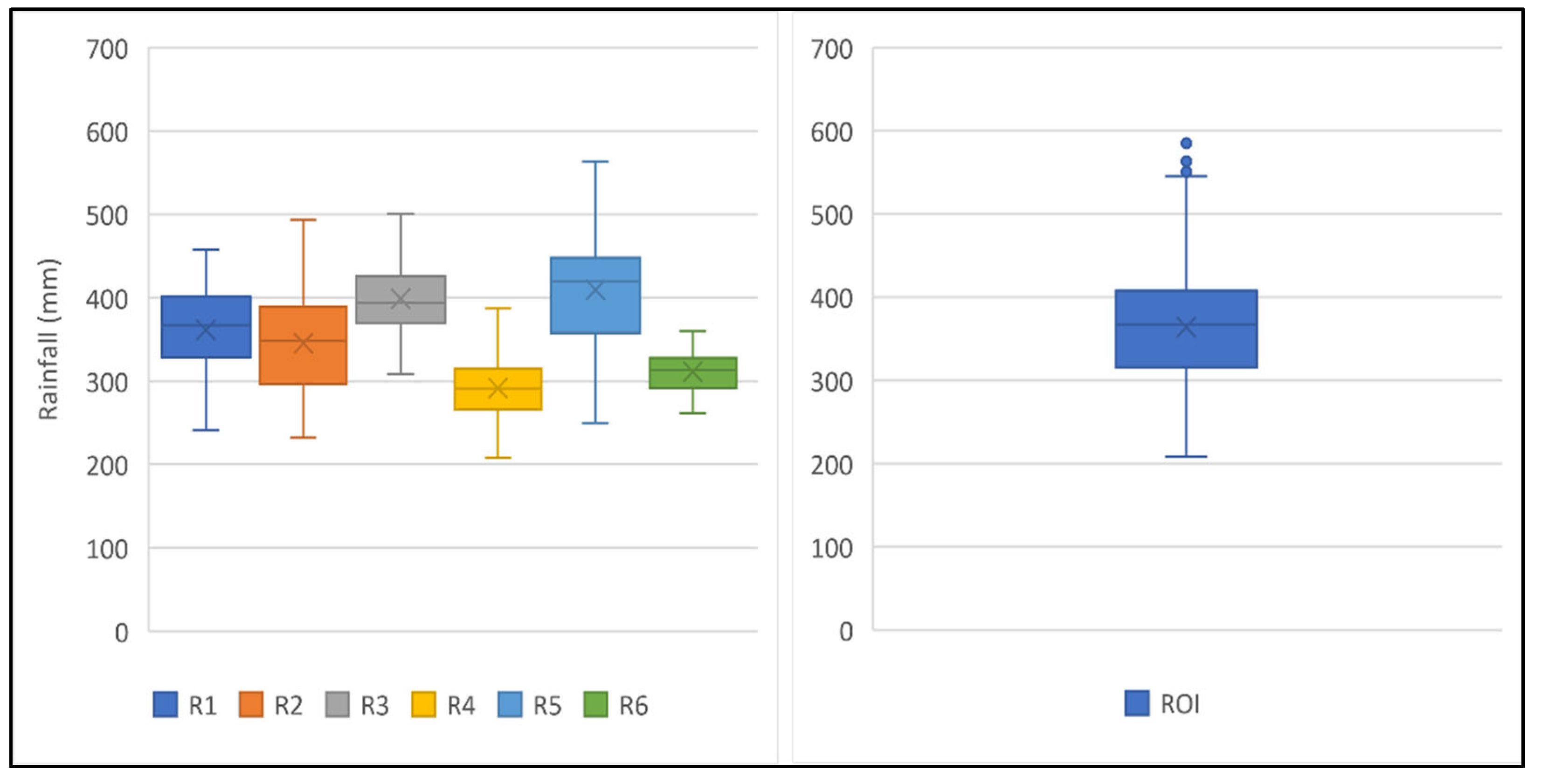
Furthermore, Figure 14 and Table 4 compare the average extreme rainfall value, standard deviation, and coefficient of variation of the RoI’s six homogeneous sub-regions and the entire RoI for the 5-year return period. The coefficient of variation value for each sub-region within the RoI is markedly different, and when compared to the CV value for the entire RoI, the CV value for each sub-region is lower. This demonstrates that the regionalization was accurate and consistent.
4. Conclusions
Regional frequency analysis of extreme rainfall was done in Taiwan using the QPESUMS daily rainfall dataset from 2006 to 2020. Taiwan was divided into 22 sub-regions based on extreme rainfall (series mean annual maximum and 5-year rainfall) and location index using K-means clustering (including latitude, longitude, and altitude). With higher radar rainfall resolution, clustering produces homogeneous regions that are not only similar, but also more detailed with clear boundaries between regions, especially in the center/mountain range area where rain stations were still limited. With Di = 6, 171 of 22,787 grids (0.75%) were discordant. Taiwan’s south-eastern coastal grid with a discordant value of 6 affects the region’s homogeneity. Based on L-moment ratio diagrams and z-values, Wakeby (WAK), GEV, and GPA extreme rainfall distributions are best for most subregions (goodness-of-fit measures). In the central and eastern regions, the Wakeby distribution is dominant and best-fitting. Estimating rainfall quantiles based on the best-fitted distribution for each sub-region increased the range of variation from 0.80–0.99 to 1.71–3.35 in a 100-year return period. This result explains why quantile estimate variation increases with return period. Sub-regions 1, 7, 11, and 22 have the highest regional growth curves in the higher return period, while sub-regions 13, 19, and 20 have the lowest. The relative regional RMSE values and 90% error bounds show that regional quantile uncertainty increases with return period, demonstrating that quantile estimations are accurate when return periods are less than 100 years. The index-flood method was used to create the spatial distribution of rainfall quantiles for several return periods (2 years, 5 years, 10 years, 20 years, 50 years, and 100 years), considering the regional growth curve as a regional scale and the annual maximum rainfall as site-specific. Two areas receive significantly more extreme rainfall than others. The southern region (sub-regions 10, 14, 15, 19, and 20) is in Tainan City, Chiayi County, Kaohsiung City, and Pingtung County. Regional frequency analysis may yield more precise estimates of rainfall quantiles than at-site analysis, not only for larger areas but also for smaller-scale areas. A region of interest has been established to determine if regionalization in the north is accurate. Each sub-coefficient regions of variation is lower than the entire RoI’s. The regionalization was accurate and consistent. According to the findings, the use of radar-rainfall in the estimation of extreme rainfall using a regional approach is highly recommended in other regions with unreliable or relatively few and uneven rain gauges, particularly in catchment areas that require frequency analysis for water-related infrastructure that is typically not covered by sufficient rain gauges.
Supplementary Materials
The following supporting information can be downloaded at: https://www.mdpi.com/article/10.3390/w14172710/s1, Figure S1: L-moment ratio diagram (LMRD) of 22 homogeneous regions in Taiwan (the gray dots are site sample L-moment ratios, the red points are the regional average L-moment ratios, and colored curves represent theoretical L-moment ratio curves of 5 candidate distributions); Table S1: Quantile estimates with different return periods for each homogeneous sub-region; Table S2: RMSE and 90 % error bounds of 22 homogeneous sub-regions with different return periods.
Author Contributions
Conceptualization, C.-H.C. and R.R.; methodology, C.-H.C., R.R., S.-J.W. and C.-T.H.; software, R.R. and C.-T.H.; validation, C.-H.C. and S.-J.W.; formal analysis, C.-H.C., R.R. and S.-J.W.; investigation, C.-H.C. and R.R.; resources, C.-H.C.; data curation, R.R.; writing—original draft preparation, C.-H.C. and R.R.; writing—review and editing, C.-H.C., R.R. and S.-J.W.; visualization, R.R.; supervision, C.-H.C., S.-J.W. and C.-T.H. All authors have read and agreed to the published version of the manuscript.
Funding
This research received no external funding.
Institutional Review Board Statement
Not applicable.
Informed Consent Statement
Not applicable.
Data Availability Statement
Data used in this study are duly available from the first authors on reasonable request.
Acknowledgments
This research was funded by the National Taipei University of Technology.
Conflicts of Interest
The authors declare no conflict of interest.
References
- Overeem, A. Climatology of Extreme Rainfall from Rain Gauges and Weather Radar; Wageningen University: Wageningen, The Netherlands, 2009. [Google Scholar]
- Chang’A, L.B.; Kijazi, A.L.; Mafuru, K.B.; Nying’Uro, P.A.; Ssemujju, M.; Deus, B.; Kondowe, A.L.; Yonah, I.B.; Ngwali, M.; Kisama, S.Y.; et al. Understanding the Evolution and Socio-Economic Impacts of the Extreme Rainfall Events in March-May 2017 to 2020 in East Africa. Atmos. Clim. Sci. 2020, 10, 553–572. [Google Scholar] [CrossRef]
- Rahman, H.T.; Mia, E.; Ford, J.D.; Robinson, B.E.; Hickey, G.M. Livelihood exposure to climatic stresses in the north-eastern floodplains of Bangladesh. Land Use Policy 2018, 79, 199–214. [Google Scholar] [CrossRef]
- Wei, L.; Hu, K.-H.; Hu, X.-D. Rainfall occurrence and its relation to flood damage in China from 2000 to 2015. J. Mt. Sci. 2018, 15, 2492–2504. [Google Scholar] [CrossRef]
- Alias, N.E.B. Improving Extreme Precipitation Estimates Considering Regional Frequency Analysis. Ph.D. Thesis, Kyoto University, Kyoto, Japan, 2014. [Google Scholar] [CrossRef]
- Liu, J.; Doan, C.D.; Liong, S.-Y.; Sanders, R.; Dao, A.T.; Fewtrell, T. Regional frequency analysis of extreme rainfall events in Jakarta. Nat. Hazards 2015, 75, 1075–1104. [Google Scholar] [CrossRef]
- Feng, Z.; Leung, L.R.; Hagos, S.; Houze, R.A.; Burleyson, C.D.; Balaguru, K. More frequent intense and long-lived storms dominate the springtime trend in central US rainfall. Nat. Commun. 2016, 7, 13429. [Google Scholar] [CrossRef]
- Fawad, M.; Yan, T.; Chen, L.; Huang, K.; Singh, V.P. Multiparameter probability distributions for at-site frequency analysis of annual maximum wind speed with L-Moments for parameter estimation. Energy 2019, 181, 724–737. [Google Scholar] [CrossRef]
- Harka, A.E.; Jilo, N.B.; Behulu, F. Spatial-temporal rainfall trend and variability assessment in the Upper Wabe Shebelle River Basin, Ethiopia: Application of innovative trend analysis method. J. Hydrol. Reg. Stud. 2021, 37, 100915. [Google Scholar] [CrossRef]
- Kim, D.-I.; Han, D.; Lee, T. Reanalysis Product-Based Nonstationary Frequency Analysis for Estimating Extreme Design Rainfall. Atmosphere 2021, 12, 191. [Google Scholar] [CrossRef]
- Tung, Y.-S.; Wang, C.-Y.; Weng, S.-P.; Yang, C.-D. Extreme index trends of daily gridded rainfall dataset (1960–2017) in Taiwan. Terr. Atmos. Ocean. Sci. 2022, 33, 8. [Google Scholar] [CrossRef]
- Mamoon, A.A.; Rahman, A. Uncertainty Analysis in Design Rainfall Estimation Due to Limited Data Length: A Case Study in Qatar. In Extreme Hydrology and Climate Variability; Elsevier Inc.: Amsterdam, The Netherlands, 2019. [Google Scholar] [CrossRef]
- Su, B.; Kundzewicz, Z.; Jiang, T. Simulation of extreme precipitation over the Yangtze River Basin using Wakeby distribution. Theor. Appl. Climatol. 2009, 96, 209–219. [Google Scholar] [CrossRef]
- Gaál, L.; Kyselý, J.; Szolgay, J. Region-of-influence approach to a frequency analysis of heavy precipitation in Slovakia. Hydrol. Earth Syst. Sci. 2008, 12, 825–839. [Google Scholar] [CrossRef]
- Hosking, J.R.M.; Wallis, J.R. Regional Frequency Analysis; Cambridge University Press: Cambridge, UK, 1997. [Google Scholar] [CrossRef]
- Greenwood, J.A.; Landwehr, J.M.; Matalas, N.C.; Wallis, J.R. Probability weighted moments: Definition and relation to parameters of several distributions expressable in inverse form. Water Resour. Res. 1979, 15, 1049–1054. [Google Scholar] [CrossRef]
- Hosking, J.R.M. L-Moments: Analysis and Estimation of Distributions Using Linear Combinations of Order Statistics. J. R. Stat. Soc. Ser. B (Methodol.) 1990, 52, 105–124. [Google Scholar] [CrossRef]
- Eldardiry, H.; Habib, E. Examining the Robustness of a Spatial Bootstrap Regional Approach for Radar-Based Hourly Precipitation Frequency Analysis. Remote Sens. 2020, 12, 3767. [Google Scholar] [CrossRef]
- Li, M.; Li, X.; Ao, T. Comparative Study of Regional Frequency Analysis and Traditional At-Site Hydrological Frequency Analysis. Water 2019, 11, 486. [Google Scholar] [CrossRef]
- Gaál, L.; Kyselý, J. Comparison of region-of-influence methods for estimating high quantiles of precipitation in a dense dataset in the Czech Republic. Hydrol. Earth Syst. Sci. 2009, 13, 2203–2219. [Google Scholar] [CrossRef]
- Malekinezhad, H.; Nachtnebel, H.; Klik, A. Comparing the index-flood and multiple-regression methods using L-moments. Phys. Chem. Earth Parts A/B/C 2011, 36, 54–60. [Google Scholar] [CrossRef]
- Gado, T.; Hsu, K.; Sorooshian, S. Rainfall frequency analysis for ungauged sites using satellite precipitation products. J. Hydrol. 2017, 554, 646–655. [Google Scholar] [CrossRef]
- Modarres, R.; Sarhadi, A. Statistically-based regionalization of rainfall climates of Iran. Glob. Planet. Chang. 2011, 75, 67–75. [Google Scholar] [CrossRef]
- Santos, M.; Fragoso, M.; Santos, J.A. Regionalization and susceptibility assessment to daily precipitation extremes in mainland Portugal. Appl. Geogr. 2017, 86, 128–138. [Google Scholar] [CrossRef]
- Yin, Y.; Chen, H.; Xu, C.-Y.; Xu, W.; Chen, C.; Sun, S. Spatio-temporal characteristics of the extreme precipitation by L-moment-based index-flood method in the Yangtze River Delta region, China. Theor. Appl. Climatol. 2016, 124, 1005–1022. [Google Scholar] [CrossRef]
- Mulaomerović-Šeta, A.; Blagojević, B.; Imširović, Š.; Nedić, B. Assessment of Regional Analyses Methods for Spatial Interpolation of Flood Quantiles in the Basins of Bosnia and Herzegovina and Serbia. In Lecture Notes in Networks and Systems; Springer: Berlin, Germany, 2022; Volume 316. [Google Scholar] [CrossRef]
- Overeem, A.; Buishand, T.A.; Holleman, I. Extreme rainfall analysis and estimation of depth-duration-frequency curves using weather radar. Water Resour. Res. 2009, 45, W10424. [Google Scholar] [CrossRef]
- Sarmadi, F.; Shokoohi, A. Regionalizing precipitation in Iran using GPCC gridded data via multivariate analysis and L-moment methods. Theor. Appl. Climatol. 2015, 122, 121–128. [Google Scholar] [CrossRef]
- Goudenhoofdt, E.; Delobbe, L.; Willems, P. Regional frequency analysis of extreme rainfall in Belgium based on radar estimates. Hydrol. Earth Syst. Sci. 2017, 21, 5385–5399. [Google Scholar] [CrossRef]
- Yeh, H.-F.; Chang, C.-F. Using Standardized Groundwater Index and Standardized Precipitation Index to Assess Drought Characteristics of the Kaoping River Basin, Taiwan. Water Resour. 2019, 46, 670–678. [Google Scholar] [CrossRef]
- Wu, C.-C.; Kuo, Y.-H. Typhoons Affecting Taiwan: Current Understanding and Future Challenges. Bull. Am. Meteorol. Soc. 1999, 80, 67–80. [Google Scholar] [CrossRef]
- Chen, H.-W.; Chen, C.-Y. Warning Models for Landslide and Channelized Debris Flow under Climate Change Conditions in Taiwan. Water 2022, 14, 695. [Google Scholar] [CrossRef]
- Chang, F.-J.; Chiang, Y.-M.; Tsai, M.-J.; Shieh, M.-C.; Hsu, K.-L.; Sorooshian, S. Watershed rainfall forecasting using neuro-fuzzy networks with the assimilation of multi-sensor information. J. Hydrol. 2014, 508, 374–384. [Google Scholar] [CrossRef]
- Chiou, P.T.; Chen, C.-R.; Chang, P.-L.; Jian, G.-J. Status and outlook of very short range forecasting system in Central Weather Bureau, Taiwan. In Applications with Weather Satellites II; SPIE: Washington, DC, USA, 2005; pp. 185–196. [Google Scholar] [CrossRef]
- Chang, R.-C.; Tsai, T.-S.; Yao, L. Intelligent Rainfall Monitoring System for Efficient Electric Power Transmission. In Information Technology Convergence; Springer: Dordrecht, The Netherlands, 2013; pp. 773–782. [Google Scholar] [CrossRef]
- Neykov, N.M.; Neytchev, P.N.; Van Gelder, P.H.A.J.M.; Todorov, V.K. Robust detection of discordant sites in regional frequency analysis. Water Resour. Res. 2007, 43, W06417. [Google Scholar] [CrossRef]
- Hosking, J.R.M. Regional Frequency Analysis Using L-Moments. 2019. Available online: https://cran.r-project.org/package=lmomRFA (accessed on 12 July 2021).
- Lin, G.-F.; Chen, L.-H. Identification of homogeneous regions for regional frequency analysis using the self-organizing map. J. Hydrol. 2006, 324, 1–9. [Google Scholar] [CrossRef]
- Alem, A.M.; Tilahun, S.A.; Moges, M.A.; Melesse, A.M. A regional hourly maximum rainfall extraction method for part of Upper Blue Nile Basin, Ethiopia. In Extreme Hydrology and Climate Variability; Elsevier: Amsterdam, The Netherlands, 2019; pp. 93–102. [Google Scholar] [CrossRef]
- Rao, A.R.; Srinivas, S.S. Regionalization of Watersheds: An Approach Based on Cluster Analysis; Springer Science & Business Media: Berlin, Germany, 2008. [Google Scholar] [CrossRef]
- Abdi, A.; Hassanzadeh, Y.; Talatahari, S.; Fakheri-Fard, A.; Mirabbasi, R. Regional drought frequency analysis using L-moments and adjusted charged system search. J. Hydroinformatics 2017, 19, 426–442. [Google Scholar] [CrossRef]
- Wright, M.J.; Houck, M.H.; Ferreira, C.M. Discriminatory Power of Heterogeneity Statistics with Respect to Error of Precipitation Quantile Estimation. J. Hydrol. Eng. 2015, 20, 04015011. [Google Scholar] [CrossRef]
- Khan, S.A.; Hussain, I.; Hussain, T.; Faisal, M.; Muhammad, Y.S.; Shoukry, A.M. Regional Frequency Analysis of Extremes Precipitation Using L-Moments and Partial L-Moments. Adv. Meteorol. 2017, 2017, 6954902. [Google Scholar] [CrossRef]
- Busababodhin, P.; Seo, Y.A.; Park, J.-S.; Kumphon, B.-O. LH-moment estimation of Wakeby distribution with hydrological applications. Stoch. Environ. Res. Risk Assess. 2016, 30, 1757–1767. [Google Scholar] [CrossRef]
- Rahman, M.; Hassan, R.; Buyya, R. Jaccard Index based availability prediction in enterprise grids. Procedia Comput. Sci. 2010, 1, 2707–2716. [Google Scholar] [CrossRef]
- Chang, P.-L.; Zhang, J.; Tang, Y.-S.; Tang, L.; Lin, P.-F.; Langston, C.; Kaney, B.; Chen, C.-R.; Howard, K. An Operational Multi-Radar Multi-Sensor QPE System in Taiwan. Bull. Am. Meteorol. Soc. 2021, 102, E555–E577. [Google Scholar] [CrossRef]
- Hu, C.; Xia, J.; She, D.; Xu, C.; Zhang, L.; Song, Z.; Zhao, L. A modified regional L-moment method for regional extreme precipitation frequency analysis in the Songliao River Basin of China. Atmos. Res. 2019, 230, 104629. [Google Scholar] [CrossRef]
- Chen, L.-H.; Hong, Y.-T. Regional Taiwan rainfall frequency analysis using principal component analysis, self-organizing maps and L-moments. Hydrol. Res. 2012, 43, 275–285. [Google Scholar] [CrossRef]
- Szolgay, J.; Parajka, J.; Kohnová, S.; Hlavčová, K. Comparison of mapping approaches of design annual maximum daily precipitation. Atmos. Res. 2009, 92, 289–307. [Google Scholar] [CrossRef]
- Rossi, F.; Fiorentino, M.; Versace, P. Two-Component Extreme Value Distribution for Flood Frequency Analysis. Water Resour. Res. 1984, 20, 847–856. [Google Scholar] [CrossRef]
- Gabriele, S.; Arnell, N. A hierarchical approach to regional flood frequency analysis. Water Resour. Res. 1991, 27, 1281–1289. [Google Scholar] [CrossRef]
- De Luca, D.L.; Galasso, L. Stationary and Non-Stationary Frameworks for Extreme Rainfall Time Series in Southern Italy. Water 2018, 10, 1477. [Google Scholar] [CrossRef] [Green Version]
- Hao, W.; Hao, Z.; Yuan, F.; Ju, Q.; Hao, J. Regional Frequency Analysis of Precipitation Extremes and Its Spatio-Temporal Patterns in the Hanjiang River Basin, China. Atmosphere 2019, 10, 130. [Google Scholar] [CrossRef]
- Beguería, S.; Vicente-Serrano, S.M. Mapping the Hazard of Extreme Rainfall by Peaks over Threshold Extreme Value Analysis and Spatial Regression Techniques. J. Appl. Meteorol. Clim. 2006, 45, 108–124. [Google Scholar] [CrossRef]
- Prudhomme, C.; Reed, D.W. Mapping Extreme Rainfall in a Mountainous Region Using Geostatistical Techniques: A Case Study in Scotland. Int. J. Climatol. 1999, 19, 1337–1356. [Google Scholar] [CrossRef]
- Su, S.-H.; Kuo, H.-C.; Hsu, L.-H.; Yang, Y.-T. Temporal and Spatial Characteristics of Typhoon Extreme Rainfall in Taiwan. J. Meteorol. Soc. Jpn. Ser. II 2012, 90, 721–736. [Google Scholar] [CrossRef]
- Malekinezhad, H.; Zare-Garizi, A. Regional frequency analysis of daily rainfall extremes using L-moments approach. Atmósfera 2014, 27, 411–427. [Google Scholar] [CrossRef]
- Wang, Z.; Zeng, Z.; Lai, C.; Lin, W.; Wu, X.; Chen, X. A regional frequency analysis of precipitation extremes in Mainland China with fuzzy c-means and L-moments approaches. Int. J. Clim. 2017, 37, 429–444. [Google Scholar] [CrossRef]
Figure 1.
The study area and the location of radars.

Figure 2.
Flowchart of Regional Frequency Analysis using L-Moments.

Figure 3.
Site-characteristics used in K-means clustering (Latitude and Longitude, Elevation, The average of Annual Maximum Series, and 5-year Rainfall.
Figure 3.
Site-characteristics used in K-means clustering (Latitude and Longitude, Elevation, The average of Annual Maximum Series, and 5-year Rainfall.

Figure 4.
Spatial distribution of QPESUMS discordant grids in Taiwan; (a). Discordant grids using Di > 3 as critical; (b). L-skewness and L-CV plot for Di > 3 (red dots represent discordant grids); (c). Discordant grids using Di > 6; (d). L-skewness and L-CV plot for Di > 6 (red dots represent discordant grids).

Figure 5.
Discordant grids along the coastal in comparison with three closest rain gauges.

Figure 6.
The division of 22 homogeneous subregions using QPESUMS in Comparison with Chen and Hong, (2012) [48]’s homogeneous subregions using Rain Gauges in Taiwan.
Figure 6.
The division of 22 homogeneous subregions using QPESUMS in Comparison with Chen and Hong, (2012) [48]’s homogeneous subregions using Rain Gauges in Taiwan.

Figure 7.
Regional growth curves of 22 homogeneous regions in Taiwan.

Figure 8.
Spatial patterns of extreme rainfall for different return periods.

Figure 9.
Touqian Watershed as region for comparing regional and grid-based (at-site) analysis.

Figure 10.
Extreme rainfall for at-site frequency analysis using the GEV distribution and regional frequency analysis at 50-year return period.
Figure 10.
Extreme rainfall for at-site frequency analysis using the GEV distribution and regional frequency analysis at 50-year return period.

Figure 11.
Comparison of the average extreme rainfall for at-site and regional frequency analysis at 50-year return period.
Figure 11.
Comparison of the average extreme rainfall for at-site and regional frequency analysis at 50-year return period.

Figure 12.
Similarity index for Touqian and Taiwan.

Figure 13.
Region of Interest in Northern part of Taiwan used for spatial investigation.

Figure 14.
Extreme rainfall of six sub-regions within region of interest and the whole region of interest at 5-year.
Figure 14.
Extreme rainfall of six sub-regions within region of interest and the whole region of interest at 5-year.


Table 1.
L-moment ratios and heterogeneity measure of 22 subregions.
| Region/Sub-Region | Number of Grids | L-Moment Ratios | H1 | ||
|---|---|---|---|---|---|
| t | t_3 | t_4 | |||
| North | |||||
| 1 | 711 | 0.33 | 0.24 | 0.17 | −2.01 |
| 2 | 453 | 0.22 | 0.21 | 0.11 | −0.62 |
| 3 | 509 | 0.19 | 0.18 | 0.15 | −0.67 |
| 4 | 1359 | 0.25 | 0.28 | 0.17 | −0.14 |
| 5 | 1806 | 0.28 | 0.15 | 0.10 | −1.86 |
| 6 | 606 | 0.24 | 0.20 | 0.16 | −1.27 |
| West | |||||
| 7 | 980 | 0.32 | 0.34 | 0.17 | −5.83 |
| 8 | 1186 | 0.26 | 0.19 | 0.10 | −5.33 |
| 9 | 1961 | 0.27 | 0.26 | 0.20 | −7.71 |
| 10 | 1150 | 0.26 | 0.25 | 0.14 | 0.85 |
| Center | |||||
| 11 | 1938 | 0.32 | 0.29 | 0.08 | −4.97 |
| 12 | 1344 | 0.25 | 0.11 | 0.10 | −4.90 |
| 13 | 826 | 0.23 | 0.00 | 0.06 | −6.01 |
| 14 | 474 | 0.22 | 0.07 | 0.05 | −1.19 |
| 15 | 567 | 0.17 | 0.11 | 0.20 | −6.87 |
| East | |||||
| 16 | 2231 | 0.25 | 0.08 | 0.06 | −5.21 |
| 17 | 652 | 0.25 | 0.17 | 0.09 | 0.07 |
| South | |||||
| 18 | 1629 | 0.19 | 0.09 | 0.12 | −3.63 |
| 19 | 609 | 0.16 | 0.10 | 0.12 | −6.49 |
| 20 | 1283 | 0.16 | 0.05 | 0.08 | −3.25 |
| 21 | 265 | 0.25 | 0.20 | 0.07 | −2.55 |
| 22 | 248 | 0.35 | 0.30 | 0.14 | 0.92 |
Table 2.
GoF measures (Z-test), best fit Distribution, and parameter distribution of 22 homogenous Sub-Regions in Taiwan.
Table 2.
GoF measures (Z-test), best fit Distribution, and parameter distribution of 22 homogenous Sub-Regions in Taiwan.
| Reg | Goodness-of-Fit Measures | Best Fit Distribution | Parameter Estimates for Distributions Accepted at the 0.90 Level | ||||||||
|---|---|---|---|---|---|---|---|---|---|---|---|
| GLO | GEV | GNO | PE3 | GPA | ξ/μ | α/σ | K/β | γ | δ | ||
| North | |||||||||||
| 1 | 7.44 | 0.61 | −2.28 | −7.59 | −16.25 | GEV | 0.71 | 0.42 | −0.11 | ||
| 2 | 18.58 | 11.54 | 9.70 | 5.99 | −4.92 | WAK | 0.48 | 0.68 | 0.32 | 0.00 | 0.00 |
| 3 | 7.45 | −0.08 | −1.17 | −3.90 | −16.92 | GEV | 0.84 | 0.27 | −0.01 | ||
| 4 | 13.00 | 5.05 | −0.08 | −9.14 | −15.97 | GNO | 0.88 | 0.38 | −0.58 | ||
| 5 | 34.65 | 17.03 | 16.09 | 11.85 | −20.90 | WAK | 0.30 | 1.04 | 0.49 | 0.00 | 0.00 |
| 6 | 5.87 | −1.60 | −3.35 | −7.00 | −18.90 | GEV | 0.79 | 0.33 | −0.05 | ||
| West | |||||||||||
| 7 | 19.51 | 14.45 | 8.66 | −1.41 | −0.68 | GPA | 0.37 | 0.62 | −0.02 | ||
| 8 | 31.21 | 18.77 | 16.39 | 11.10 | −9.58 | WAK | 0.35 | 0.58 | 2.62 | 0.58 | −0.17 |
| 9 | 1.52 | −7.88 | −13.01 | −22.24 | −33.28 | GLO | 0.89 | 0.24 | −0.26 | ||
| 10 | 19.89 | 11.13 | 7.17 | −0.05 | −10.72 | PE3 | 1.00 | 0.50 | 1.48 | ||
| Center | |||||||||||
| 11 | 63.27 | 53.04 | 45.54 | 32.36 | 25.38 | WAK | 0.32 | 0.74 | 0.10 | 0.00 | 0.00 |
| 12 | 30.61 | 13.51 | 14.22 | 11.95 | −21.70 | WAK | 0.24 | 2.03 | 7.43 | 0.70 | −0.34 |
| 13 | 35.70 | 16.95 | 21.79 | 21.79 | −16.88 | WAK | 0.18 | 2.61 | 8.57 | 0.92 | −0.69 |
| 14 | 29.02 | 16.95 | 18.71 | 18.19 | −6.53 | WAK | 0.36 | 0.92 | 1.90 | 0.42 | −0.30 |
| 15 | −11.39 | −20.36 | −19.99 | −21.20 | −38.83 | WAK | 0.40 | 2.43 | 5.54 | 0.20 | 0.11 |
| East | |||||||||||
| 16 | 56.21 | 32.30 | 34.29 | 32.08 | −15.90 | WAK | 0.26 | 1.17 | 5.37 | 0.83 | −0.50 |
| 17 | 24.58 | 14.92 | 13.61 | 10.26 | −6.62 | WAK | 0.36 | 0.56 | 2.58 | 0.58 | −0.21 |
| South | |||||||||||
| 18 | 23.65 | 1.61 | 5.38 | 3.62 | −36.65 | GEV | 0.86 | 0.30 | 0.12 | ||
| 19 | 12.97 | 1.83 | 2.73 | 1.61 | −20.65 | PE3 | 1.00 | 0.29 | 0.60 | ||
| 20 | 37.51 | 16.77 | 20.29 | 19.72 | −23.01 | WAK | 0.50 | 1.00 | 2.47 | 0.25 | −0.16 |
| 21 | 20.74 | 14.78 | 13.42 | 10.58 | 1.01 | GPA | 0.41 | 0.79 | 0.34 | ||
| 22 | 13.01 | 9.74 | 7.04 | 2.33 | 0.68 | GPA | 0.28 | 0.77 | 0.07 | ||
Table 3.
Similarity index between grid-based and regional frequency analysis for Touqian watershed and Taiwan.
Table 3.
Similarity index between grid-based and regional frequency analysis for Touqian watershed and Taiwan.
| Return Period | Touqian | Taiwan | ||
|---|---|---|---|---|
| NCC | JSI | NCC | JSI | |
| 2-year | 0.980 | 0.935 | 0.977 | 0.917 |
| 5-year | 0.989 | 0.916 | 0.965 | 0.912 |
| 10-year | 0.990 | 0.914 | 0.946 | 0.899 |
| 20-year | 0.990 | 0.888 | 0.929 | 0.890 |
| 50-year | 0.990 | 0.858 | 0.907 | 0.880 |
| 100-year | 0.989 | 0.839 | 0.892 | 0.874 |
| 1000-year | 0.988 | 0.795 | 0.849 | 0.855 |
Table 4.
Extreme rainfall statistics of six sub-regions within region of interest and the whole region of interest.
Table 4.
Extreme rainfall statistics of six sub-regions within region of interest and the whole region of interest.
| Sub-Region | Region of Interest | Whole ROI | ||||
|---|---|---|---|---|---|---|
| Mean | Std Dev | CV | Mean | Std Dev | CV | |
| 1 | 361.51 | 49.78 | 13.77 | 363.95 | 67.23 | 18.47 |
| 2 | 345.39 | 59.00 | 17.08 | |||
| 3 | 399.03 | 38.45 | 9.64 | |||
| 4 | 291.57 | 35.03 | 12.01 | |||
| 5 | 409.32 | 63.94 | 15.62 | |||
| 6 | 311.17 | 23.14 | 7.44 | |||
Publisher’s Note: MDPI stays neutral with regard to jurisdictional claims in published maps and institutional affiliations. |
© 2022 by the authors. Licensee MDPI, Basel, Switzerland. This article is an open access article distributed under the terms and conditions of the Creative Commons Attribution (CC BY) license (https://creativecommons.org/licenses/by/4.0/).
Share and Cite
MDPI and ACS Style
Chang, C.-H.; Rahmad, R.; Wu, S.-J.; Hsu, C.-T. Spatial Frequency Analysis by Adopting Regional Analysis with Radar Rainfall in Taiwan. Water 2022, 14, 2710. https://doi.org/10.3390/w14172710
AMA Style
Chang C-H, Rahmad R, Wu S-J, Hsu C-T. Spatial Frequency Analysis by Adopting Regional Analysis with Radar Rainfall in Taiwan. Water. 2022; 14(17):2710. https://doi.org/10.3390/w14172710
Chicago/Turabian StyleChang, Che-Hao, Riki Rahmad, Shiang-Jen Wu, and Chih-Tsung Hsu. 2022. "Spatial Frequency Analysis by Adopting Regional Analysis with Radar Rainfall in Taiwan" Water 14, no. 17: 2710. https://doi.org/10.3390/w14172710
Note that from the first issue of 2016, this journal uses article numbers instead of page numbers. See further details here.