
Numerical Simulation Research on the Diversion Characteristics of a Trapezoidal Channel
Key Laboratory of Agricultural Soil and Water Engineering in Arid and Semiarid Areas, Ministry of Education, Northwest A&F University, Yangling 712100, China
*
Author to whom correspondence should be addressed.
Water 2022, 14(17), 2706; https://doi.org/10.3390/w14172706
Submission received: 14 July 2022
/
Revised: 22 August 2022
/
Accepted: 27 August 2022
/
Published: 30 August 2022
(This article belongs to the Section Hydraulics and Hydrodynamics)
Abstract
:Open-channel bifurcations are the most common water diversion structures in irrigation districts. In irrigation water conveyance, water transport efficiency and sedimentation are primary concerns. This study accordingly analyzes the influence of open-channel bifurcations on water delivery in irrigation areas. Herein, the three-dimensional flow at an open-channel bifurcation was studied via numerical simulations using FLOW-3D software and including 15 sets of working conditions. The hydraulic characteristics of the recirculation zone and flow structures in the vicinity of the open-channel bifurcation were analyzed. Equations for the flow diversion width of the surface and bottom layers in the trapezoidal channel were then obtained. The flow diversion widths along the water depth were found to differ between trapezoidal and rectangular channels. The results also show that open-channel bifurcations considerably influence the flow velocity in the main channel. The flow velocity in the recirculation zone of open-channel bifurcations was small, but the pulsation velocity and the turbulent kinetic energy were large. The energy dissipated in this area was relatively large, which was not conducive to channel water delivery. This study provides a reference for channel optimization and operation management in irrigation districts.
1. Introduction
Diversion channels or river bifurcations are commonly found in natural rivers as a result of the rivers’ dynamics processes [1,2]. Moreover, branch channels are commonly used for water diversion in irrigation networks, domestic use and hydropower projects [3,4,5]. The point at which the main and branch channels meet is called an open-channel bifurcation. Understanding and predicting flow properties at an open-channel bifurcation are important for accurately measuring branch flow discharge, which is necessary for agricultural irrigation and water use scheduling.
The largest body of research on open-channel bifurcations has addressed rectangular channels because they have a simple structure and are easy to measure. The rectangular channel diversion equations are the emphasis of the study. Many investigators have used theoretical analysis methods including a magnitude analysis, the momentum theorem, or energy equation to calculate the rectangular channel diversion equations [6,7,8,9]. These equations match well with experimental results and can be used for actual flow measurement. Meanwhile, with improvements in measurement instruments, research on water flow at open-channel bifurcations has expanded. Laser speed detector (LDA), acoustic doppler velocimeter (ADV) and particle image velocimetry (PIV) systems have considerably improved the measurement accuracy of water flow velocity [10,11,12,13,14]. Under these approaches, open-channel bifurcation flow patterns are first reduced into flow velocity measurements and turbulence characteristics in three dimensions. Then, according to the flow pattern of the open-channel bifurcation, a mathematical description of flow is precisely partitioned [15,16]. The formation and development of recirculation zones have also been explored for their narrowing effects on the inlet branch channel. Studies of physical quantities such as the Reynolds shear stress and turbulent viscosity have further improved the understanding of turbulence in open-channel bifurcations [17,18]. These studies provide an understanding of turbulence in bifurcations. Numerical simulation methods have advanced the understanding of branch channel flow by expanding beyond the limits of field experiments. There exist both mature commercial and self-programmed software packages with improved algorithms for simulating fluids [19,20]. Currently, the most widely used method for numerically simulating open-channel bifurcations is the Reynolds Average Navier–Stokes (RANS) method [21,22]. Among models that use RANS, the most widely adopted is the renormalization group k-ε (RNG k-ε) model. Both methods have been shown to be capable of simulating measured water depth and velocity in river and open-channel water diversions. The literature shows that the RNG k-ε model is widely used in bifurcation studies, and its reliability has been tested [23,24,25,26].
However, the shapes of many open-channel bifurcations vary from the widely researched rectangular shape due to different practical engineering needs [27,28]. In the water diversion and transportation systems in an irrigation area, channel sections are mostly trapezoidal. In such systems, flow diversion sluices are set at the water diversions to control the branch channel flow discharge. These sluices are typically rectangular. Therefore, regardless of the shape of the branch channel section, its inlet is rectangular. In the diversion sections of irrigation systems, the upper layer of clear water is often used to ensure water quality. Accordingly, the elevation of the bottom of the branch channel is higher than that in the main channel, forming a bottom sill. Due to the complex structure of the trapezoidal channel diversions, few studies have been carried out on the flow conditions under these geometries.
In this study, experimental and numerical simulations of an open-channel bifurcation with a bottom sill were accordingly conducted using a trapezoidal main channel and a rectangular branch channel inlet without sluice gates. The main objective of the current study, which is drawn from the above literature review, was to investigate the flow diversion characteristics in trapezoidal channels with different discharge from the main channel and bed widths. Another objective of the study was to find the law of variation of flow diversion widths in trapezoidal channels and compare it with the rectangular channels.
2. Methods
2.1. Experimental Setup
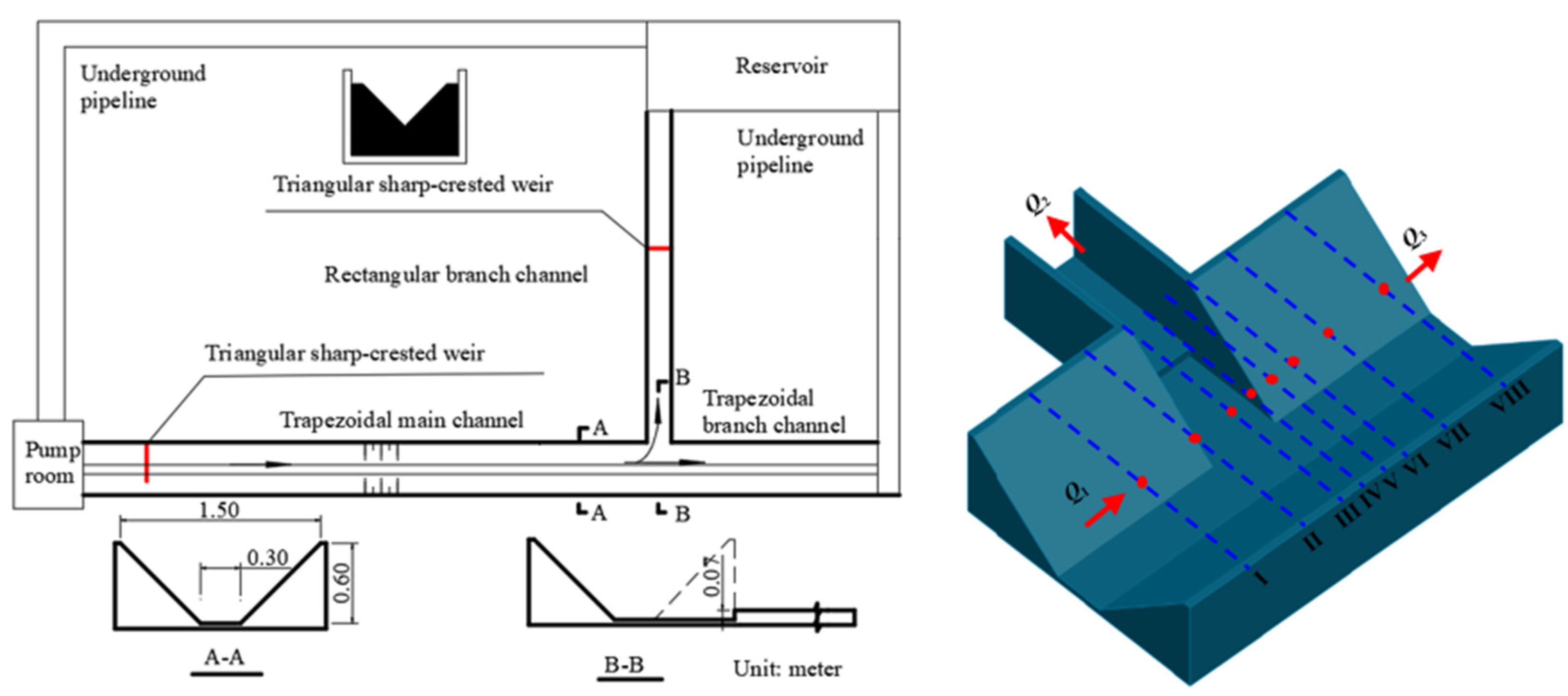
The experiments were performed at the Key Laboratory of Agricultural Soil and Water Engineering in Arid and Semiarid Areas, Northwest A&F University. The experimental system comprised a pump room, triangular sharp-crest weir, trapezoidal channel, rectangular channel, reservoir, and underground pipeline. The experimental plan layout is shown in Figure 1. The ends of the channels were governed by free outflow. Triangular sharp-crested weirs were set at the trapezoidal channel inlet and rectangular branch channel outlet to measure flow. The trapezoidal channel length was 30 m, the bottom width was 0.3 m, the height was 0.6 m, and the bank slope coefficient was 1.0. The trapezoidal channel in the upstream part of the open-channel bifurcation was called the trapezoidal main channel, and the flow discharge was Q1; the downstream of the open-channel bifurcation was called the trapezoidal branch channel, and the flow discharge was Q3. The elevation of the bottom of the trapezoidal branch channel was consistent with that of the bottom of the trapezoidal main channel. The rectangular branch channel was 8 m long, with a width of 0.36 m, and a channel height of 0.6 m, and the flow discharge was Q2. The elevation of the bottom of the rectangular branch channel was higher than the elevation of the bottom of the trapezoidal main channel, resulting in a bottom sill of 7 cm. This bottom sill was set in the rectangular branch channel 60 cm downstream at the rectangular branch channel inlet. In this channel system, the open-channel bifurcation was 20 m away from the trapezoidal main channel head, ensuring uniform flow conditions at the branch channel. The angle between the central axis of the rectangular branch channel and the central axis of the trapezoidal channel was 90°. The roughness of both channels was 0.011. Measurements were collected in the experiments at five different trapezoidal main channel flow discharges. The water depth was measured using SCM 60 needle water-level gauges with an accuracy of ±0.1 mm (manufactured by Weifang Jinshui Huayu Information Technology CO., Ltd., Weifang City, China.).
2.2. Numerical Simulation Model
Computational fluid dynamics (CFD) uses software to simulate a complex model by applying the physical conservation law of the model to establish governing equations and model-specific nonlinear partial differential equations for numerical calculations. The flow simulations in this study used the mass conservation and momentum conservation equations.
In this study, FLOW-3D software was used for the numerical simulations. FLOW-3D used the improved Tru-VOF algorithm to capture the interface between the water and gas phases to accurately simulate the flow problem with a free interface.
2.3. Governing Equations
It was assumed that the fluid used in this study was incompressible with a constant density ρ and under steady-state conditions. The fluid can thus be described by the mass conservation equation and the momentum conservation equation as follows:
where i and j represent tensor forms with a range of values of (1, 2, 3); if the experiment water temperature is 20 °C, incompressible, and if the viscosity is constant, .
For turbulent flow, the RNG k-ε model was chosen for this study. The RNG k-ε model is based on the theory of the renormalization group to build a modified equation of the standard model, which reflects the effects of small-scale vortices through large-scale turbulent eddies and modified viscosity terms. The small-scale motion is removed from the governing equations, and the rotation and swirling flows are reflected in the mean flow. Therefore, this model is suitable for flows with a large degree of curvature in the open-channel bifurcation. The k equation and the ε equation are as follows:
where k is the turbulent kinetic energy; ε is the turbulent energy dissipation rate; in which μ is the hydrodynamic viscosity coefficient and μt is the fluid turbulent viscosity; Gk is the turbulent kinetic energy k generation term due to the average velocity gradient; with αk = αε = 1.39, C1ε* = 1.42, and C2ε = 1.68, all being empirical constants.
2.4. Open-Channel Bifurcation Structure and Boundary Conditions
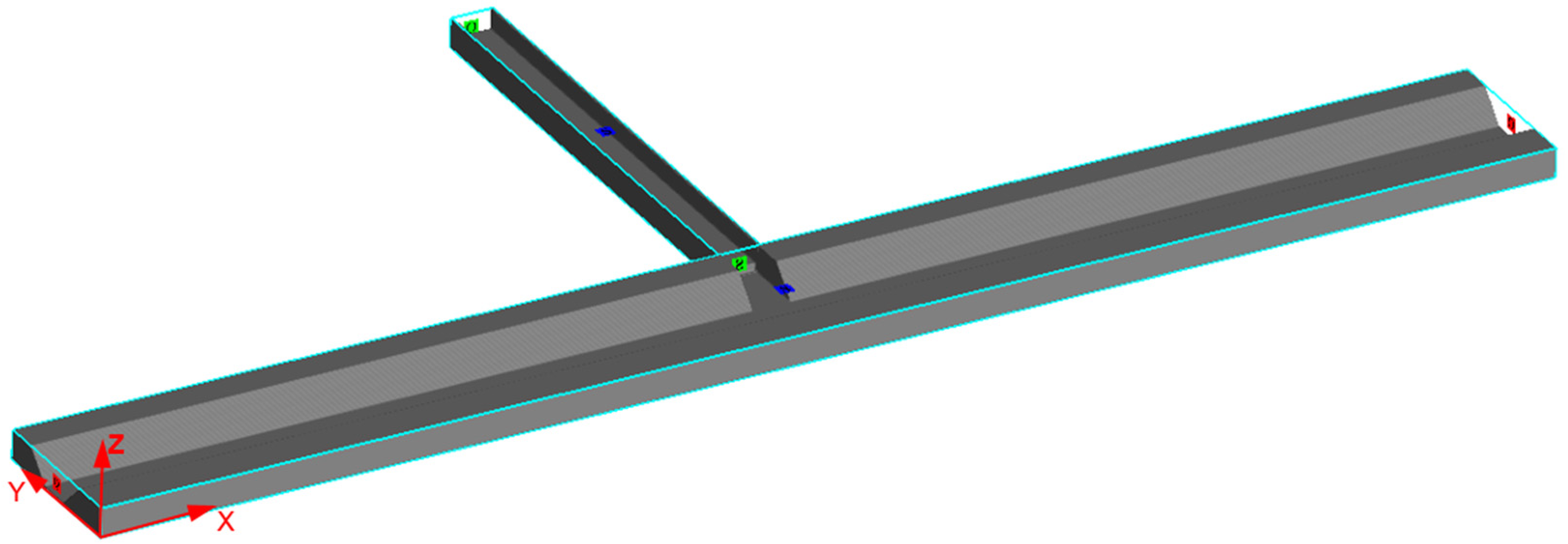
As shown in Figure 2, a numerical model of a trapezoidal channel with a rectangular open-channel bifurcation was designed to match the experimental conditions. Under fixed working conditions, the open-channel water flow developed into a uniform flow. The upstream of the trapezoidal main channel was set as the flow discharge inlet. The downstream of the trapezoidal branch channel and the downstream of the rectangular branch channel were set to free outflow. The mesh surface that was in contact with the wall of the channel was set as a wall boundary. Because the upper grid was designed higher than the water depth to account for the air, we set a symmetry boundary at the top of the grid. The normal derivative of a physical quantity was zero at the symmetry boundary. The origin of the coordinates was defined at the bottom of the channel head.
2.5. Meshing and Simulation Conditions
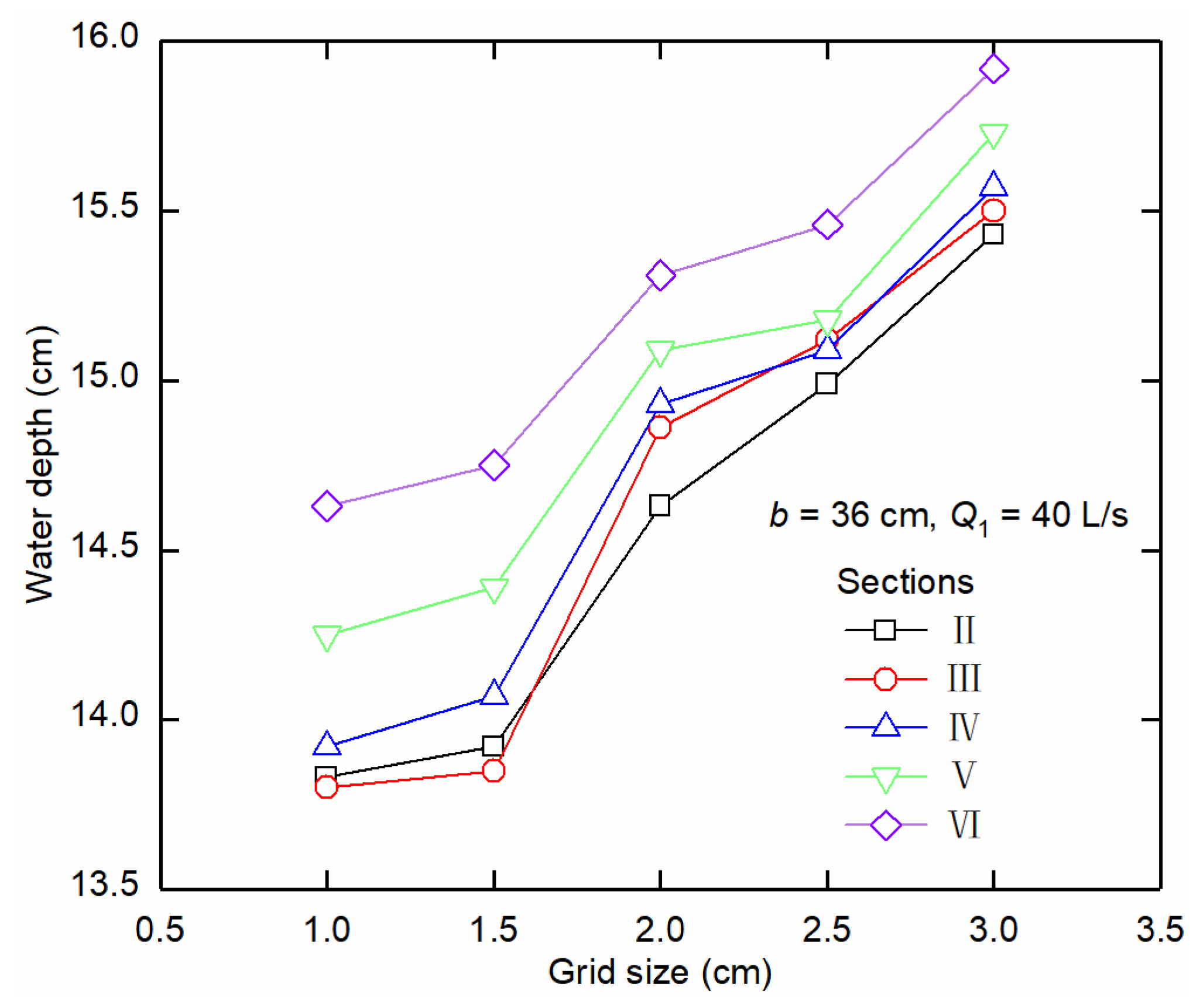
Under fixed working conditions, in order to reduce the influence of the mesh size setting on the numerical simulation results, mesh independence verification is required. For a channel width of 1.5 m, simulation meshing blocks set at 1.0, 1.5, 2.0, 2.5, or 3.0 cm were used to simulate the open-channel water flow. Figure 3 shows the simulated water depths of the measuring points on the central axis of the section at different grid sizes.
Under the same working condition, a water depth simulation value decreases as the grid size decreases, and after the grid size is less than 1.5 cm, it remains basically the same. It is shown that the effect of grid size on simulation results is negligible when the grid size is less than 1.5 cm. To ensure the accuracy of the simulation data, a 1-cm grid was used for the calculation. Table 1 shows the comparisons of the simulated and measured water depths, in particular showing that the maximum relative error between them is less than 3%. Thus, the model can be used with confidence. The numerical simulations were then evaluated for 3 different trapezoidal main channel flows, 20, 25, 30, 35, and 40 L/s, and three rectangular branch channel widths, 30, 36, and 40 cm.
3. Results and Discussion
3.1. Water Depth
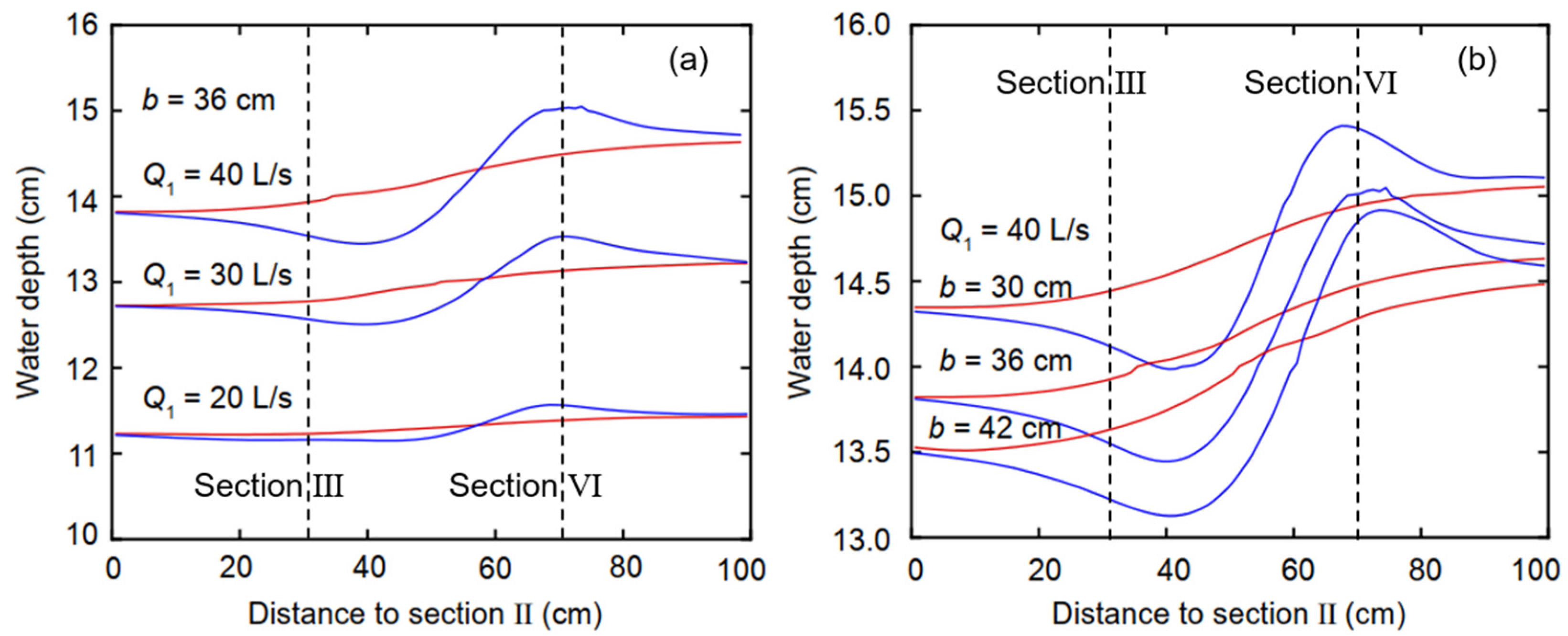
The water surface line (water depth) is the primary basis for determining the height of the open channel’s side wall, and it can directly reflect changes in water flow pattern. The observed water depth changes were concentrated near the open-channel bifurcation. The water surface curve was drawn according to the water depth at Sections II–VII of the main channel. The variations in water surface lines near the open-channel bifurcation are similar. In Figure 4, the abscissa represents the distance from the measuring point to Section II. The red lines indicate the water depth on the line y = 64 cm in the trapezoidal channel away from the open-channel bifurcation, and the blue lines indicate the water depth on the line y = 94 cm in the trapezoidal channel near the open-channel bifurcation. Figure 4a shows that the variation in water depth in the trapezoidal channel is basically the same at different flow discharges. From upstream of the open-channel bifurcation towards downstream, the water surface exhibited an initial decrease and subsequent increase as a portion of the water flowed into the rectangular channel. Figure 4b shows that the variations in the water depth in the trapezoidal channel are the same at different branch channel widths. The relatively small width of the rectangular branch channel and small flow into it is one of the main reasons for the deeper water depth in the trapezoidal channel than in the rectangular channel at the same flow discharge. As can be seen in Figure 4, changing the width of the branch channel has a greater effect on the change in water depth in the diversion area than changing the incoming flow of the main channel. Therefore, when constructing the main and branch channels in an irrigation area, the design of the channel height should take full account of the influence of the channel width ratio on the flow of water.
3.2. Froude Number
The Froude number (Fr) is the ratio of viscous force to inertial force and reflects changes in water flow patterns. Sediment is not easy to settle in supercritical flow, but it may settle in subcritical flow. In this study, local Fr was extracted on the x–y plane from FLOW-3D for analysis.
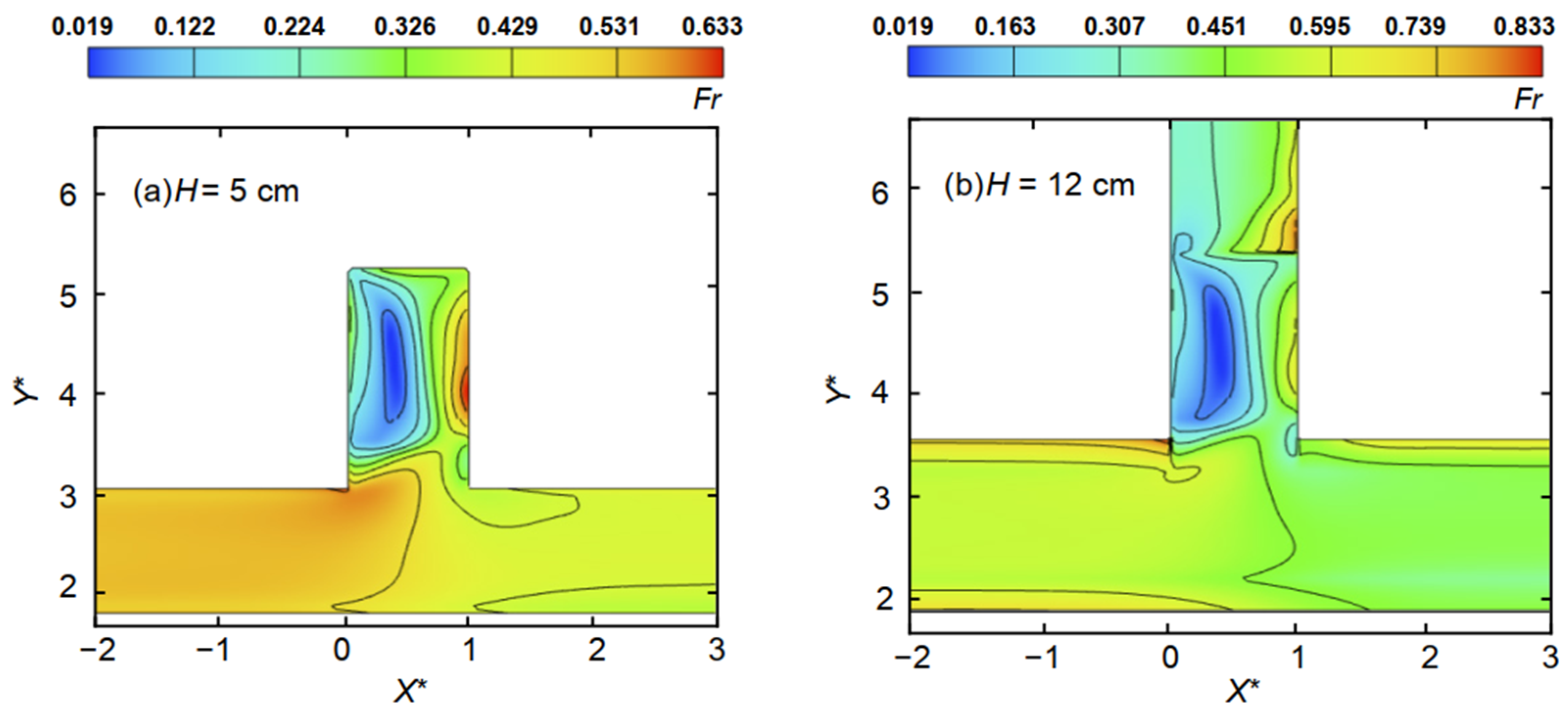
Figure 5a shows the change in Fr at a water depth of 5 cm (below the bottom sill height). There is a blue area in the rectangular branch channel called the recirculation zone. As the velocity at the center of the vortex created in this area is zero, the center of the recirculation zone has a small Fr. Flow is forced to enter the opposite (downstream) side of the branch channel because of the presence of this recirculation zone. Accordingly, the Fr is higher (as indicated by the red color) in this region, called the submerged acceleration zone. Figure 5b (at a water depth of 12 cm) shows that there is a large linear shift in Fr at the location of the bottom sill. In this region, the flow entering the rectangular branch channel is blocked by the bottom sill and its velocity increases. Flow in the rectangular branch channel is also affected by the recirculation zone and the submerged acceleration zone. Finally, the velocity upstream of the rectangular branch channel was small, but the downstream velocity in the branch channel was large.
In this study, due to the presence of the bottom sill, the recirculation zone was concentrated in the front of, rather than fully developed along, the rectangular branch channel. This makes the recirculation zone width slightly larger than in a no-bottom sill case, but its length is considerably shortened. Figure 5 shows that the range of the recirculation zone does not change much with water depth. As Fr is close to zero here at the sill, the velocity is almost zero, and the sediment in the channel is easily deposited.
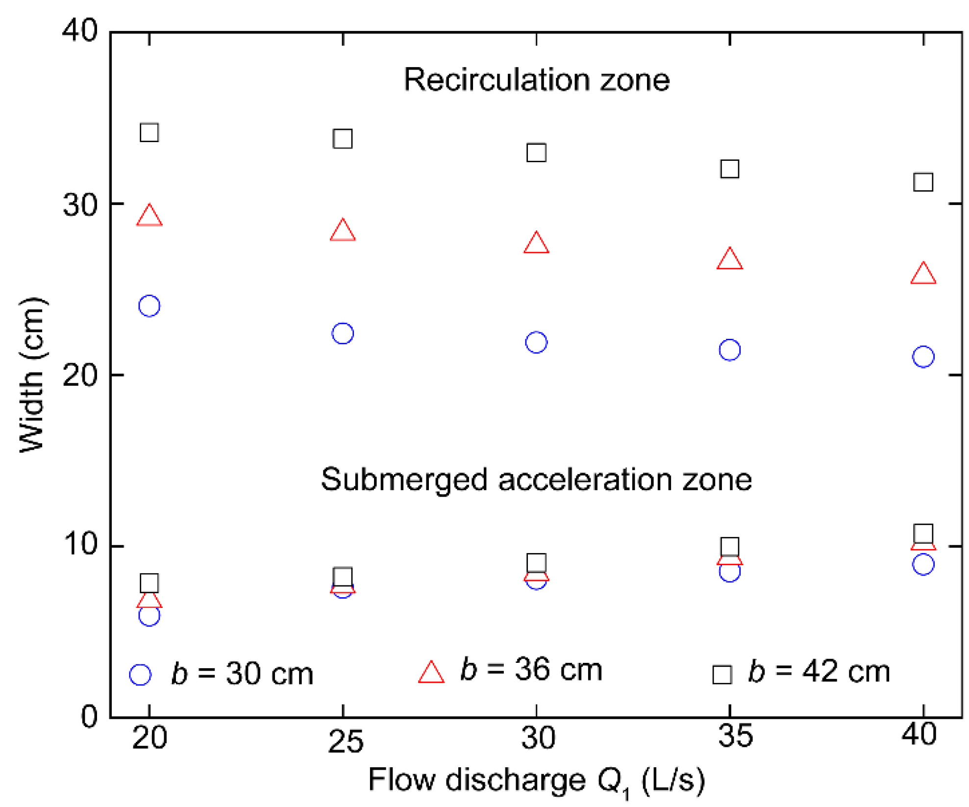
3.3. Width of the Recirculation Zone
The above analysis reveals that velocity decreases in the recirculation zone, allowing the sediment in the channel to be easily deposited. This section discusses the shape of the recirculation zone at different flow discharges and different rectangular branch widths. As the recirculation zone is restrained in front of the bottom sill, its length is fixed at 60 cm; however, the changes in its width can be studied. Figure 6 shows the widths of the recirculation and submerged acceleration zones under different operating conditions. Coordinate points of the same shape and color represent the same rectangular branch channel width. As the width rectangular branch increases, the width of the recirculation zone increases, the width of the submerged acceleration zone decreases, and the narrowing effect experienced by the water flow entering the branch channel increases.
Figure 6 shows that the width of the recirculation zone slowly decreases with increasing Q1, whereas the width of the subsurface flow acceleration zone slowly increases. Their change ranges are small, and the narrowing effect of the recirculation zone does not change significantly with the change in Q1. When Q1 is fixed, changing the rectangular branch widths return the widths of recirculation zone varies substantially. However, nearly no difference is observed in the width of the submerged acceleration zone. Therefore, the flow-narrowing effect of the recirculation zone does not change significantly with the changing rectangular branch channel width. As a result, in an open-channel bifurcation with a bottom sill fixed 60 cm from the branch inlet, the width of the submerged acceleration zone and the flow narrowing effect are almost constant under different working conditions.
3.4. Velocity Distribution in the Main Channel
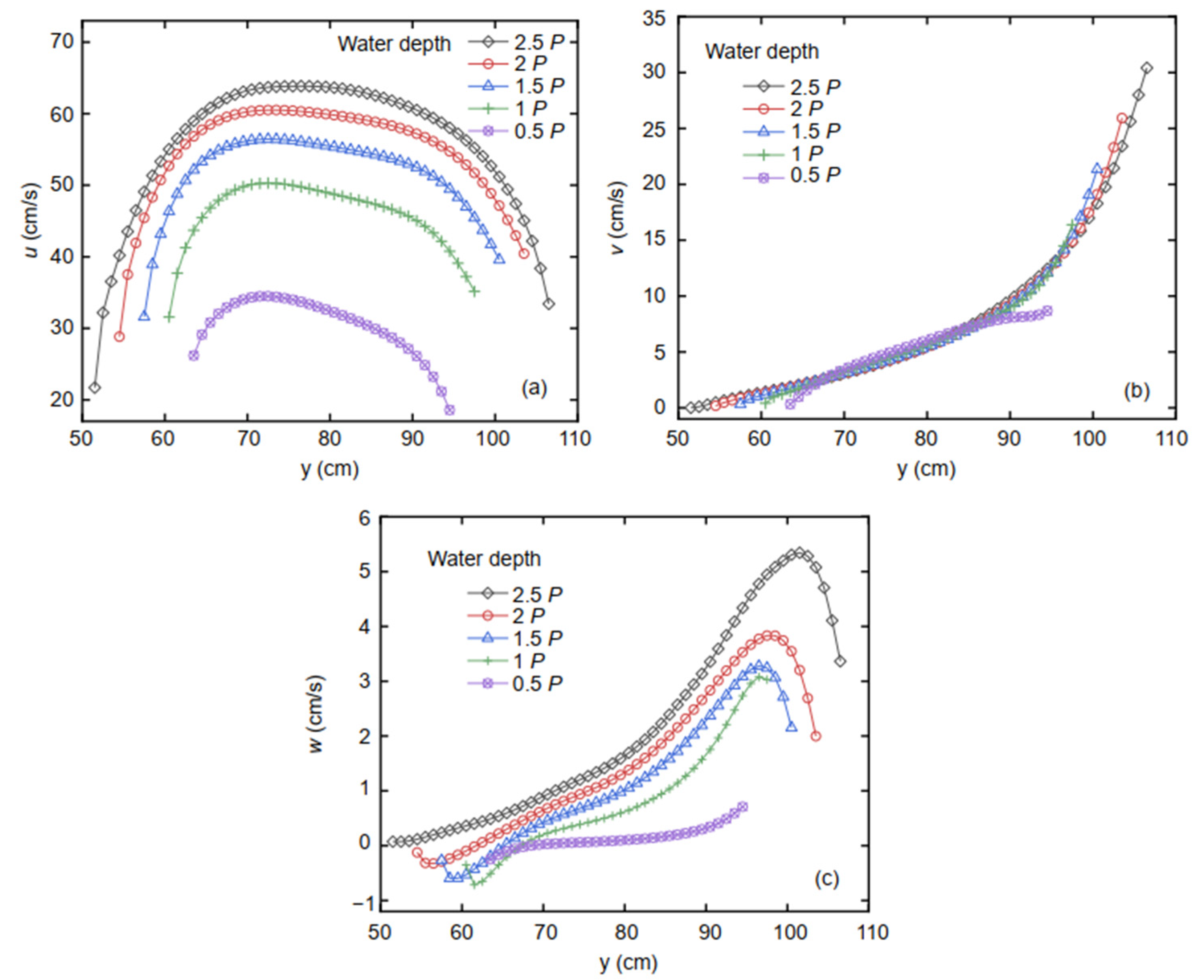
The streamlines in FLOW-3D were curved near the open-channel bifurcation in the main channel, indicating a drastic change in velocity. The region of the main channel flow diversion was divided into six zones in past research on the open-channel bifurcations of rectangular channels, such as the acceleration zone, stagnation zone, and separation deceleration zone. The velocity distributions near the open-channel bifurcation were also drawn in detail in this study. The velocity in a trapezoidal main channel is different from that in a no-bifurcation open channel, as the former has a distinct component flowing to the rectangular branch channel. When a bottom sill is set in the open-channel bifurcation, the velocity in the z-axis direction is different from that of the no-bottom sill condition. Figure 7 shows the three-dimensional flow velocity distribution at different water depths on Section Ⅴ.
Comparing the velocity changes at different water depths reveals that the velocity changes are mostly identical. The purple velocity distribution line is lower than the other lines, which are all higher than the bottom sill, and its variation law is different from that of the others. In the velocity distribution lines above the bottom sill, the left side is the wall, where the flow does not participate in the flow diversion, and the velocities u and v are the smallest. The right side is the rectangular branch channel, where the flow turns into the branch channel. Thus, the right velocity v is the maximum, whereas u is smaller. The left-center velocity u is the largest, and it gradually decreases as the y-axis coordinate increases. The open-channel bifurcation substantially influences the velocity of the main channel although the flow diversion width is not large in the main channel. For the purple velocity distribution line, the velocity u on the left side is larger than that on the right side, and velocities v and w are smaller than those on the right side, indicating that the right-side flow moved into the rectangular branch channel. Comparing the velocity in Figure 7a–c, the velocities u and w are found to be consistent with the following law: the surface velocity is larger than the bottom velocity in open channels. The velocity v is nearly identical in each layer of water at the Section V.
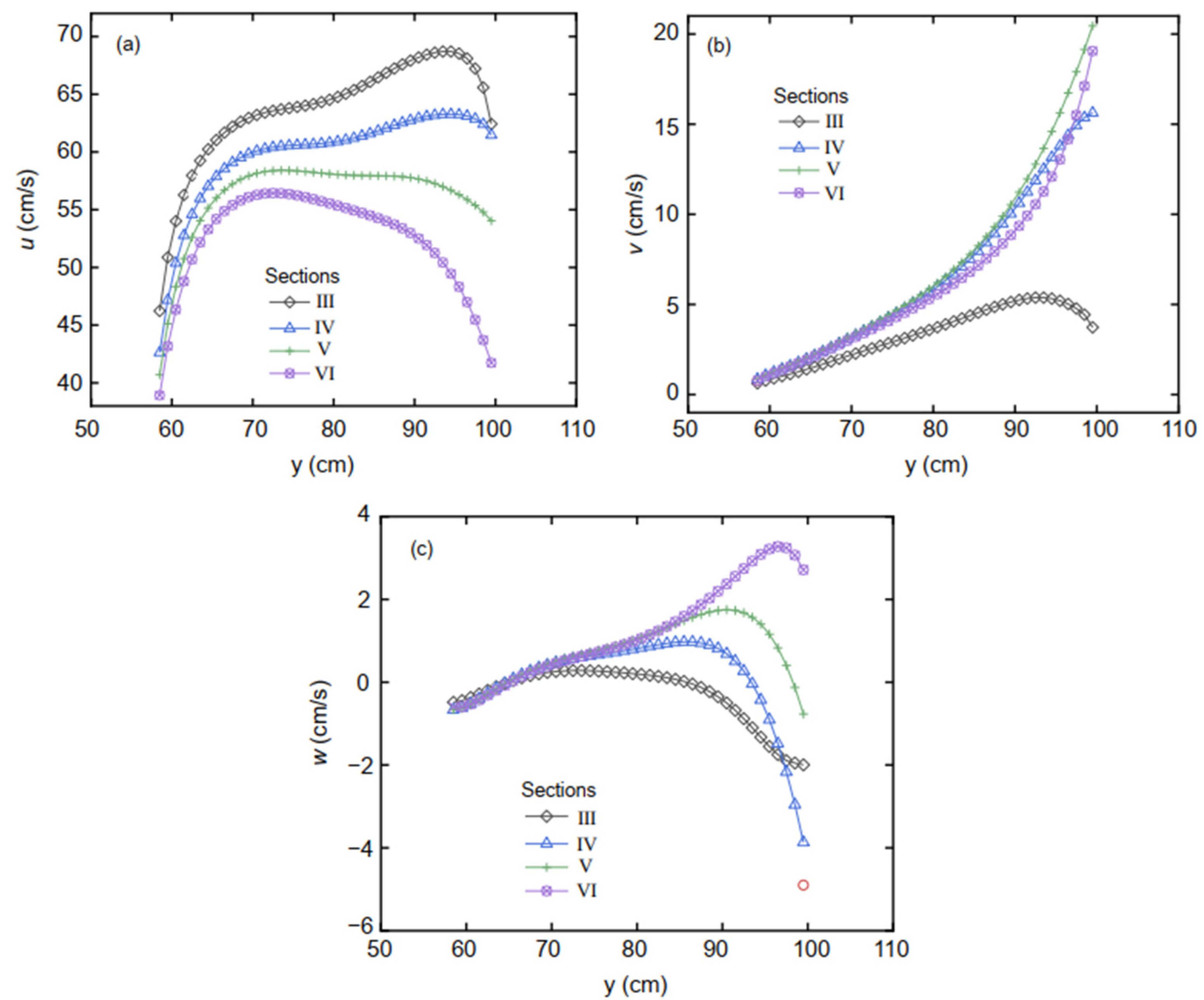
Comparing the velocity changes across different sections at a water depth of 1.5P (Figure 8) reveals the velocity variation law to be complicated. The velocity u gradually decreases along the x-axis direction in Figure 8a, reflecting the change in velocity from the acceleration zone to the separation deceleration zone in the main channel. The velocity v first increases and then decreases along the x-axis direction in Figure 8b. This indicates that the flow trends into the branch channel at the upstream lip of the open-channel bifurcation. The flow at the downstream lip of the open-channel bifurcation cannot enter the branch channel, and only the water in the main channel diffuses to the entire section and has a y-direction velocity. Three sections have negative values in Figure 8c because of a secondary circulation flow that causes a negative velocity w near the open-channel bifurcation. The existence of the open-channel bifurcation changes the distribution law of the velocity in the open channel, and thus, it plays a qualitative role in the flow measurement and sedimentation in open channels.
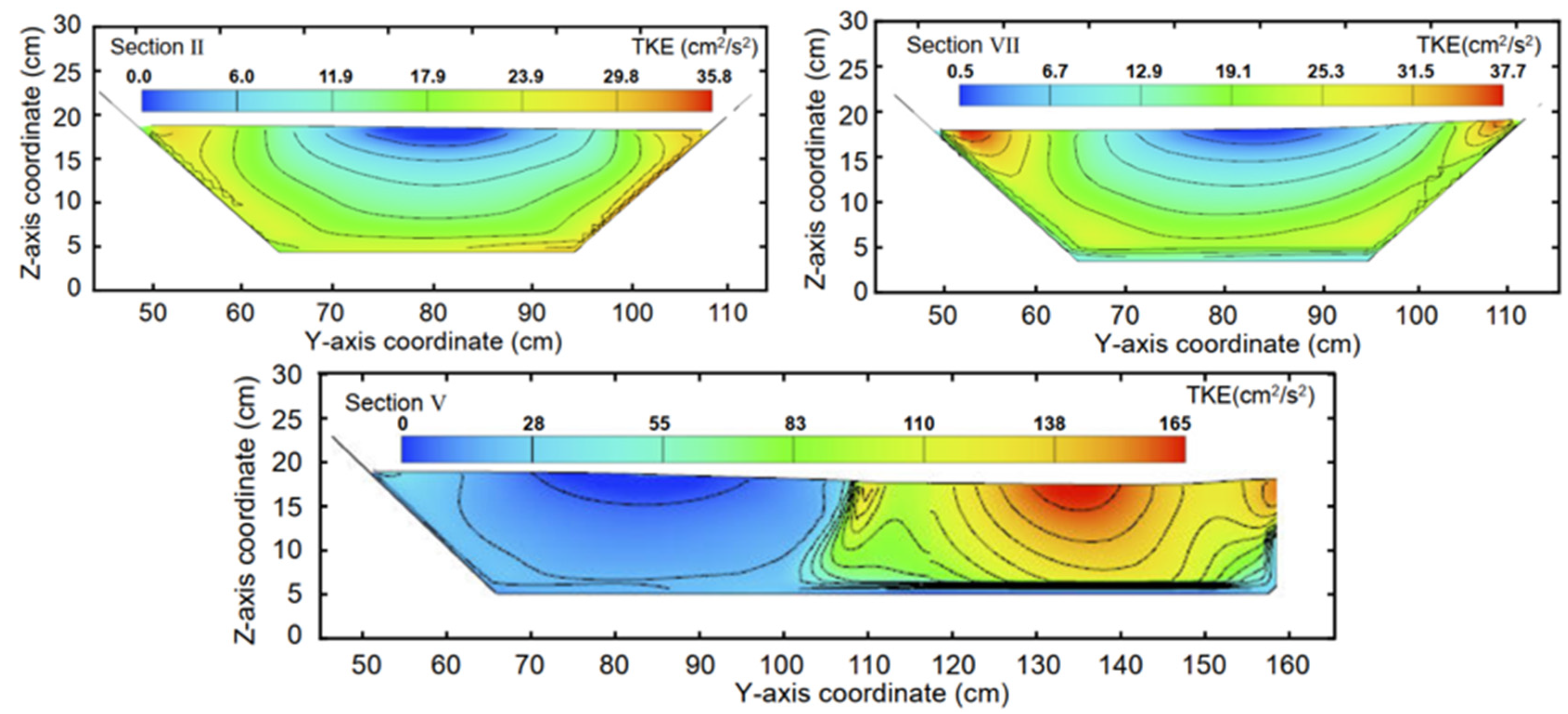
3.5. Turbulent Kinetic Energy
Turbulent energy is a physical parameter that provides an indication of the overall turbulence of the water flow and supports material transport and energy transfer. The calculation of TKE is as follows:
As can be observed in Figure 9, the TKE was generally small in both the rectangular and trapezoidal channels. The minimum TKE in the open channel was 0.075, indicating that the pulsation intensity on the water surface was not large, but the TKE in the recirculation zone was larger, followed by the submerged acceleration zone.
There are vortices of various scales in turbulent flow. A large eddy of the same order of magnitude as the flow field would cause low-frequency pulsation. The small-scale vortex formed after a large-scale vortex rupture would induce high-frequency pulsation. A large-scale vortex continuously extracts energy from the mainstream and transmits it to the small-scale vortex through their interactions. Finally, the energy is converted into heat dissipation by the viscosity of water, which causes the current-average energy to be transformed into pulsating kinetic energy and thermal energy. The obstruction of the solid boundary creates several vortices, and the recirculation zone is formed by the constraints of the bottom sill and side wall. Therefore, many vortices were formed in the recirculation zone, the pulsation velocity was large, and the TKE was as high as 203.11. Due to the narrowing effect of the recirculation zone and the side wall, many vortices were formed in the submerged acceleration region. The random motion of the vortex caused the pulsation of the physical quantity of water, resulting in a high TKE in this region. Similarly, in the trapezoidal main channel, a new vortex was created due to the obstruction of the solid boundary, and the TKE near the side wall was higher than that at the center of the channel.
3.6. Flow Diversion Width
Flow diversion width is the width at which the water enters the side channel from the main channel. The size of the flow diversion width is a direct factor determining the amount of flow into the branch channel. The flow diversion width has been studied from very early on, but primarily in rectangular channels [16]. However, the variation in the flow diversion width along the water depth in a trapezoidal channel differs from that in a rectangular channel.
The velocity at the bottom of a rectangular channel is zero, and the surface velocity is the highest, and at an open-channel bifurcation, both the surface velocity and inertial force are large. Therefore, it is easier to turn the bottom flow into the branch channel than the surface flow. Thus, in a rectangular channel, the surface water (or that slightly below the surface layer) has the smallest flow diversion width, whereas the bottom has the largest flow diversion width. However, we found that the surface flow diversion width was larger at the surface of the trapezoidal channel than at the bottom and that the flow diversion width was the smallest at 0.2–0.4 times the water depth. The difference between the trapezoidal and rectangular channels is reflected in Figure 10a. The flow discharge in the upper part of the trapezoidal channel is larger than that in the lower part, and the flow diversion in the upper part of the channel accounts for a significant proportion of the total water diversion. As the bottom inertial force is small, the bottom flow easily enters the branch channel. Therefore, the flow diversion width in the trapezoidal channel decreases from the bottom of the channel as the elevation increases to a minimum at 0.2 to 0.4 times the water depth, followed by gradual increase. Moreover, the surface flow diversion width is the largest. When the sediment is transported in the channel, it is concentrated at the bottom of the channel. Therefore, in the trapezoidal channel, the surface flow diversion dominates, and less sediment enters the branch channel than the rectangular channel.
Through the study of the flow diversion width under 15 working conditions, the surface flow and bottom flow diversion widths were determined to be related to the flow discharge in the trapezoidal main channel and the width of the rectangular branch channel as expressed by:
where Bs and Bb are the surface and bottom flow diversion widths; K1 = 4.90Q1 + 0.11 and K2 = 4.60Q1 + 0.06 in which Q1 is the flow discharge in the trapezoidal main channel in m3/s; and b is the width of the rectangular branch channel in units consistent with B. It can be seen from Figure 10b, c that the equations are in good agreement with the simulation data.
4. Conclusions
According to the structure of typical open-channel bifurcations of trapezoidal channels in irrigation areas, a bottom sill was designed in a rectangular diversion channel and the diversion law was studied based on experimentally verified numerical simulations. The results of this research suggest the following conclusions.
The RNG k-ε model in the FLOW-3D software was able to successfully simulate flow phenomena at the open-channel bifurcation, and the simulation results agreed well in comparisons with water depths from field experiment data.
The velocity was substantially affected by the open-channel bifurcation in the trapezoidal channel. Due to the characteristics of the recirculation zone and the submerged acceleration zone in the rectangular branch channel, the velocity after each zone was different.
The recirculation zone was manifested as an observable vortex that was mainly determined by boundary conditions (side wall and bottom sill). It had a near-zero center velocity, resulting in a small Fr, and a large TKE, indicating the value of pulsating velocity was large, and that the existence of the recirculation zone has a narrowing effect on the flow. This study thus concludes that the recirculation zone has a negligible narrowing effect on flow diversion at different rectangular branch widths and different flow discharges.
The flow diversion width in the trapezoidal main channel was different from that in a rectangular main channel, but little other research mentions this observation. The surface flow diversion width in the trapezoidal channel was the largest followed by the bottom flow diversion width. The flow diversion width was the smallest at a depth of 0.2 to 0.4 times the water depth. This was caused by the trapezoidal channel bank slope. In contrast, it has been previously observed that the bottom flow diversion width in the rectangular channel is the largest and that on the surface is the smallest. Thus, because sediments are concentrated at the bottom of channels, trapezoidal channels convey less sediment to branch channels. Because the flow diversion width rule of the trapezoidal channel is different from that of the rectangular channel, this study recalculated the equation for the flow diversion width at the surface and bottom layers when the channel bank slope coefficient m = 1.0.
These results can provide a reference for the simulation and design of water conveyance operations and their complex turbulent flow fields. They also provide a theoretical basis for channel optimization to reduce sediment deposition. However, further study is required to explore open-channel bifurcations at different water inlet angles as well as sandy water laws.
Author Contributions
Conceptualization, Y.C., C.L. and W.W.; methodology, Y.C. and Y.S.; software, X.H.; validation, Y.S., C.L. and W.W.; formal analysis, Y.C. and Y.S.; investigation, C.L.; resources, X.H.; data curation, Y.S. and W.W.; writing—original draft, Y.C.; writing—review and editing, W.W.; visualization, C.L.; supervision, X.H.; project administration, X.H.; funding acquisition, W.W. All authors have read and agreed to the published version of the manuscript.
Funding
This research was funded by the National Natural Science Foundation of China (52079113) and Shaanxi Province Water Conservancy Science and Technology Project (2021slkj-8).
Institutional Review Board Statement
Not applicable.
Informed Consent Statement
Not applicable.
Data Availability Statement
The data presented in this study are available on request from the corresponding author [email protected].
Conflicts of Interest
The authors declare no conflict of interest.
References
- Kleinhans, M.G.; Ferguson, R.I.; Lane, S.N.; Hardy, R.J. Splitting rivers at their seams: Bifurcations and avulsion. Earth Surf. Proc. Landf. 2013, 38, 47–61. [Google Scholar] [CrossRef]
- Redolfi, M.; Zolezzi, G.; Tubino, M. Free instability of channel bifurcations and morphodynamic influence. J. Fluid Mech. 2016, 799, 476–504. [Google Scholar] [CrossRef]
- Meselhe, E.A.; Sadid, K.M.; Allison, M.A. Riverside morphological response to pulsed sediment diversions. Geomorphology 2016, 270, 184–202. [Google Scholar] [CrossRef]
- Ahn, M.J.; Lyu, S. The impact of water-intake for a tributary on the flow and saline intrusion in the lower Han River. KSCE J. Civ. Eng. 2017, 21, 1945–1955. [Google Scholar] [CrossRef]
- Alomari, N.K.; Yusuf, B.; Mohammad, T.A.; Ghazali, A.H. Experimental investigation of scour at a channel junctions of different diversion angles and bed width ratios. Catena 2018, 166, 10–20. [Google Scholar] [CrossRef]
- Ramamurthy, A.S.; Satish, M.G. Division of flow in short open channel branches. J. Hydraul. Eng. 1988, 114, 428–438. [Google Scholar] [CrossRef]
- Lama, S.K.; Kuroki, M.; Hasegawa, K. Study of flow bifurcation at tic 30° open channel junction when the width ratio of branch channel to main channel is large. Proc. Hydraul. Eng. 2002, 46, 583–588. [Google Scholar] [CrossRef]
- Rivière, N.; Travin, G.; Perkins, R.J. Transcritical flows in three and four branch open-channel intersections. J. Hydraul. Eng. 2014, 140, 04014003. [Google Scholar] [CrossRef]
- Hsu, C.C.; Tang, C.J.; Lee, W.J.; Shieh, M.Y. Subcritical 90° equal-width open-channel dividing flow. J. Hydraul. Eng. 2002, 128, 716–720. [Google Scholar] [CrossRef]
- Neary, V.S.; Odgaard, A.J. Three-dimensional flow structure at open-channel diversions. J. Hydraul. Eng. 1993, 119, 1223–1230. [Google Scholar] [CrossRef]
- Barkdoll, B.D.; Hagen, B.L.; Odgaard, A.J. Experimental comparison of dividing open-channel with duct flow in T-junction. J. Hydraul. Eng. 1998, 124, 92–95. [Google Scholar] [CrossRef]
- Auel, C.; Albayrak, I.; Boes, R.M. Turbulence characteristics in supercritical open channel flows: Effects of Froude number and aspect ratio. J. Hydraul. Eng. 2014, 140, 040140044. [Google Scholar] [CrossRef]
- Moghadam, M.K.; Bajestan, M.S.; Sedghi, H.; Seyedian, M. An experimental and numerical study of flow patterns at a 30 degree water intake from trapezoidal and rectangular channels. Iran. J. Sci. Technol. Trans. Civ. Eng. 2014, 38, 85–97. [Google Scholar]
- Mignot, E.; Wei, C.; Launay, G.; Riviere, N.; Escauriaza, C. Coherent turbulent structures at the mixing-interface of a square open-channel lateral cavity. Phys. Fluids 2016, 28, 045104. [Google Scholar] [CrossRef]
- Abderrezzak, K.E.K.; Lewicki, L.; Paquier, A.; Riviere, N.; Travin, G. Division of critical flow at three-branch open-channel intersection. J. Hydraul. Res. 2011, 49, 231–238. [Google Scholar] [CrossRef]
- Luo, F.A.; Liang, Z.Y.; Zhang, D.R. Experimental studies on division of flow. Adv. Water Sci. 1995, 6, 71–75. [Google Scholar]
- Yang, F. Study on “Diversion Angle Effect” of Lateral Intake Flow; China Institute of Water Resources and Hydropower Research: Beijing, China, 2007; p. 29. [Google Scholar]
- Mignot, E.; Doppler, D.; Riviere, N.; Vinkovic, I.; Gence, J.N.; Simoens, S. Analysis of flow separation using a local frame axis: Application to the open-channel bifurcation. J. Hydraul. Eng. 2014, 140, 280–290. [Google Scholar] [CrossRef]
- Li, C.W.; Zeng, C. 3D Numerical modelling of flow divisions at open channel junctions with or without vegetation. Adv. Water Resour. 2009, 32, 49–60. [Google Scholar] [CrossRef]
- Hardy, R.J.; Lane, S.N.; Yu, D. Flow structures at an idealized bifurcation: A numerical experiment. Earth Surf. Proc. Landf. 2011, 36, 2083–2096. [Google Scholar] [CrossRef]
- Mignot, E.; Zeng, C.; Dominguez, G.; Li, C.W.; Rivière, N.; Bazin, P.H. Impact of topographic obstacles on the discharge distribution in open-channel bifurcations. J. Hydrol. 2013, 494, 10–19. [Google Scholar] [CrossRef]
- Khandelwal, V.; Dhiman, A.; Baranyi, L. Laminar flow of non-Newtonian shear-thinning fluids in a T-channel. Comput. Fluids 2015, 108, 79–91. [Google Scholar] [CrossRef]
- Neary, V.S.; Sotiropoulos, F.; Odgaard, A.J. Three-dimensional numerical model of lateral-intake inflows. J. Hydraul. Eng. 1999, 125, 126–140. [Google Scholar] [CrossRef]
- Huang, J.; Weber, L.J.; Lai, Y.G. Three-dimensional numerical study of flows in open-channel junctions. J. Hydraul. Eng. 2002, 128, 268–280. [Google Scholar] [CrossRef]
- Ramamurthy, A.S.; Qu, J.; Vo, D. Numerical and experimental study of dividing open-channel flows. J. Hydraul. Eng. 2007, 133, 1135–1144. [Google Scholar] [CrossRef]
- Wang, W.E.; Liu, H.Q.; Hu, X.T. Numerical simulation of influence of side channel bottom height on hydraulic performance of bleeder. Trans. Chin. Soc. Agric. Eng. 2019, 35, 60–68. [Google Scholar]
- Ku, H.C. Solution of flow in complex geometries by the pseudospectral element method. J. Comput. Phys. 1995, 117, 215–227. [Google Scholar] [CrossRef]
- Li, T.; Zou, J.; Qu, S.J.; Liu, Z.; Ren, Z.H.; Tian, W.J. Local head loss of 90° lateral diversion from open channels of different cross-sectional shapes. J. Hydroelectr. Eng. 2017, 36, 30–37. [Google Scholar]
Figure 1.
Experimental plan and section measurement layout. Note: Red points in the figure represent the measurement point arrangement, and Roman numerals represent measurement section numbers.
Figure 1.
Experimental plan and section measurement layout. Note: Red points in the figure represent the measurement point arrangement, and Roman numerals represent measurement section numbers.

Figure 2.
Numerical simulation model and boundary conditions.

Figure 3.
Grid independence test. Note: b is the branch channel width and Q1 is flow discharge in the main channel.
Figure 3.
Grid independence test. Note: b is the branch channel width and Q1 is flow discharge in the main channel.

Figure 4.
Water depth change along the direction of water flow in trapezoidal open channel for (a) variation in flow discharge and (b) variation in branch channel width. Note: Red lines indicate the water depth on the line y = 64 cm, blue lines indicate the water depth on the line y = 94 cm.
Figure 4.
Water depth change along the direction of water flow in trapezoidal open channel for (a) variation in flow discharge and (b) variation in branch channel width. Note: Red lines indicate the water depth on the line y = 64 cm, blue lines indicate the water depth on the line y = 94 cm.

Figure 5.
Froude number (Fr) contour map at different water depths. Note: Q1 = 40 L/s; b = 30 cm. X* and Y* are obtained by dimensionless processing of X-axis and Y-axis coordinates. (a) depth of water below the sill height; (b) depth of water above the sill height.
Figure 5.
Froude number (Fr) contour map at different water depths. Note: Q1 = 40 L/s; b = 30 cm. X* and Y* are obtained by dimensionless processing of X-axis and Y-axis coordinates. (a) depth of water below the sill height; (b) depth of water above the sill height.

Figure 6.
Relationships between the width of the recirculation zone, flow discharge, and rectangular channel width.
Figure 6.
Relationships between the width of the recirculation zone, flow discharge, and rectangular channel width.

Figure 7.
Velocity distribution at different water depths. Note: Q1 = 40 L/s; b = 30 cm; P = 7 cm, which is the bottom sill height. (a) The x-direction with velocity u; (b) the y-direction with velocity v; and (c) the z-direction with velocity w.
Figure 7.
Velocity distribution at different water depths. Note: Q1 = 40 L/s; b = 30 cm; P = 7 cm, which is the bottom sill height. (a) The x-direction with velocity u; (b) the y-direction with velocity v; and (c) the z-direction with velocity w.

Figure 8.
Velocity distribution at different sections. Note: Water depth of 1.5P; Q1 = 40 L/s; b = 30 cm. (a) The x-direction with velocity u; (b) the y-direction with velocity v; and (c) the z-direction with velocity w.
Figure 8.
Velocity distribution at different sections. Note: Water depth of 1.5P; Q1 = 40 L/s; b = 30 cm. (a) The x-direction with velocity u; (b) the y-direction with velocity v; and (c) the z-direction with velocity w.

Figure 9.
Turbulent kinetic energy (TKE) contour map on different sections.

Figure 10.
(a) Comparison of flow diversion widths in the trapezoidal and rectangular channels and comparisons of the calculated and simulated values of the flow diversion width for (b) surface flow and (c) bottom flow.
Figure 10.
(a) Comparison of flow diversion widths in the trapezoidal and rectangular channels and comparisons of the calculated and simulated values of the flow diversion width for (b) surface flow and (c) bottom flow.


Table 1.
Analysis of the relative error of water depth in different sections at the flow rate of 40 L/s and the branch channel width of 36 cm.
Table 1.
Analysis of the relative error of water depth in different sections at the flow rate of 40 L/s and the branch channel width of 36 cm.
| Section | Analog Value/cm | Measured Value/cm | Relative Error/% |
|---|---|---|---|
| Ⅱ | 13.83 | 13.46 | 2.75 |
| Ⅲ | 13.8 | 13.78 | 0.18 |
| Ⅳ | 13.92 | 13.93 | −0.08 |
| Ⅴ | 14.25 | 14.34 | −0.62 |
| Ⅵ | 14.63 | 14.88 | −1.66 |
| Ⅶ | 14.69 | 14.92 | −1.56 |
Publisher’s Note: MDPI stays neutral with regard to jurisdictional claims in published maps and institutional affiliations. |
© 2022 by the authors. Licensee MDPI, Basel, Switzerland. This article is an open access article distributed under the terms and conditions of the Creative Commons Attribution (CC BY) license (https://creativecommons.org/licenses/by/4.0/).
Share and Cite
MDPI and ACS Style
Cheng, Y.; Song, Y.; Liu, C.; Wang, W.; Hu, X. Numerical Simulation Research on the Diversion Characteristics of a Trapezoidal Channel. Water 2022, 14, 2706. https://doi.org/10.3390/w14172706
AMA Style
Cheng Y, Song Y, Liu C, Wang W, Hu X. Numerical Simulation Research on the Diversion Characteristics of a Trapezoidal Channel. Water. 2022; 14(17):2706. https://doi.org/10.3390/w14172706
Chicago/Turabian StyleCheng, Yong, Yude Song, Chunye Liu, Wene Wang, and Xiaotao Hu. 2022. "Numerical Simulation Research on the Diversion Characteristics of a Trapezoidal Channel" Water 14, no. 17: 2706. https://doi.org/10.3390/w14172706
Note that from the first issue of 2016, this journal uses article numbers instead of page numbers. See further details here.