


Implementation of Quantitative Resilience Measurement Criteria in Irrigation Systems
by
 and
and
Carmen Mireya Lapo Pauta
1,*,
Viviana A. Briceño Ojeda
1,
Francisco Javier Martínez-Solano
2 and
and
Holger Benavides Muñoz
1
1
Civil Engineering Department, Universidad Técnica Particular de Loja, Loja 110150, Ecuador
2
Department of Hydraulic Engineering and Environment, Universitat Politécnica de Valencia, 46022 Valencia, Spain
*
Author to whom correspondence should be addressed.
Water 2022, 14(17), 2698; https://doi.org/10.3390/w14172698
Submission received: 30 May 2022
/
Revised: 28 July 2022
/
Accepted: 3 August 2022
/
Published: 30 August 2022
(This article belongs to the Special Issue New Perspectives in Agricultural Water Management)
Abstract
:This paper shows the research developed in order to evaluate two resilience indicators, PHRI and Rsys, in the San Francisco de Cunuguachay pressurized irrigation network, specifically in the Yulchirón 2 branch. In this context, the irrigation branch was designed to operate on an on-demand basis and in shifts in order to evaluate the indicators in both operation modes, subjecting the network to unfavourable events. The resilience at the level of pressures and demands of the branch is estimated to remain operational in the different disruptive events, meeting the minimum conditions of the initial design. In this regard, with the implementation of resilience indicators in irrigation networks, it is possible to diagnose the response of the network to changes in its operation. Therefore, the use of indicators allows for obtaining a more reliable and adaptable network to changes in its operation. Consequently, the use of indicators allows for obtaining more reliable and adaptable networks to changes, since the engineer can make the right decisions in the project, improving the planning and management of irrigation networks.
1. Introduction
Irrigation systems are closely linked to development at socio-organisational, agro-productive and economic improvement levels then their multifunctional character is evident. Nonetheless, irrigation involves high water consumption. The Food and Agriculture Organization of the United Nations [1] indicates that agriculture accounts for approximately 70% of the world’s freshwater withdrawals, and in some developing countries this can be as high as 95%. Due to projected world population growth, it is estimated that by the year 2050, a 60% increase in agricultural production will be necessary, and consequently the water requirement for agriculture will also increase; however, by optimising irrigation practices, this expected increase could be reduced to only 10%. [1,2].
In Ecuador, irrigation accounts for 71.2% of freshwater withdrawals. In 2010, the demand for irrigation was 13,045 hm3, it is expected to increase by 22.4 % by 2025. Currently, approximately 1,528,474 ha are under irrigation, but due to the condition of the existing infrastructure, the effective irrigation rate is only 64%. To ensure sustainable production and to avoid the negative effects of water stress, efficient irrigation systems and their proper management are required [3]. Ministry of Agriculture, Livestock, Aquaculture and Fisheries (MAGAP, in its original Spanish) [4] affirms that the comprehensive design and management of irrigation projects in Ecuador is a challenge that needs to be addressed.
In this context, the concept of resilience can be an appropriate tool for the planning and management of irrigation systems, as it allows for more adaptable and reliable water infrastructure [5]; although in engineering this concept is relatively new in relation to other fields [6], there is no universal definition of the concept of resilience. Nevertheless, many researchers, such as Liu et al. [7] and Butler et al. [8], indicate that it is the ability of the system to cope with and respond to unfavourable events (e.g., operational changes, pipe ruptures, pressure drops, etc.). Ayala Cabrera et al. [9] claims that resilience indicators provide useful information for better preparedness (planning) and management (mitigation) during unfavourable situations in water networks.
The purpose of this research is to answer the question: Does the implementation of quantitative resilience indicators in irrigation networks allow us to evaluate the robustness of the network in the face of disruptive events? Therefore, two resilience indicators will be evaluated in the “San Francisco de Cunuguachay” irrigation network, a sector located in the province of Chimborazo. The selected indicators were: (i) the “Pipeline Hydraulic Resilience Index (PHRI)” of Liu et al. [10] and (ii) the “adaptability index” of Zhuan et al. (2012) quoted in Shin et al. [5], where the aim is to improve decision making with regard to the planning and management of this irrigation system in the event of unfavourable events.
In order to achieve this, the response of the network is determined when it is subjected to various unfavourable scenarios (changes in network operation, pressure variations, variations in demand); however, assessing all the scenarios is complicated as many are probabilistic, or events that may possibly occur in response to changes in its operation. For the development of the research work, first, the continuous fictitious flow is calculated referring to Smith et al. [11] based on the agronomic requirements of the network. The irrigation network is designed to operate on-demand according to Clement, 1966, cited in Lamaddalena and Sagardoy, [12] and operates in shifts in accordance with Lapo Pauta et al. [13]. In the hydraulic design of the irrigation network, the hydraulic parameters are verified. Finally, the resilience indexes described above are implemented and calculated for the study network.
2. Methodology
2.1. Field of Study
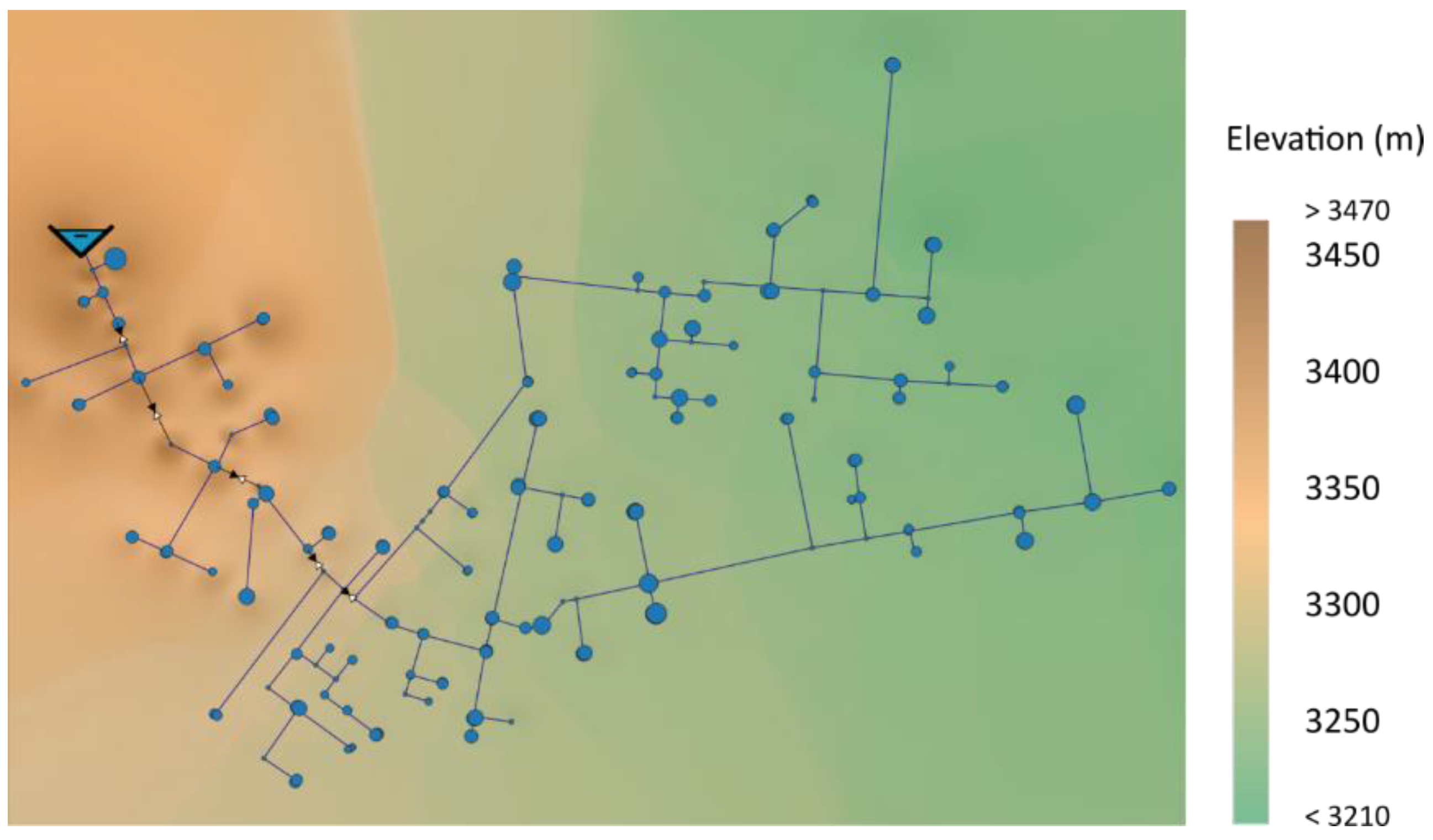
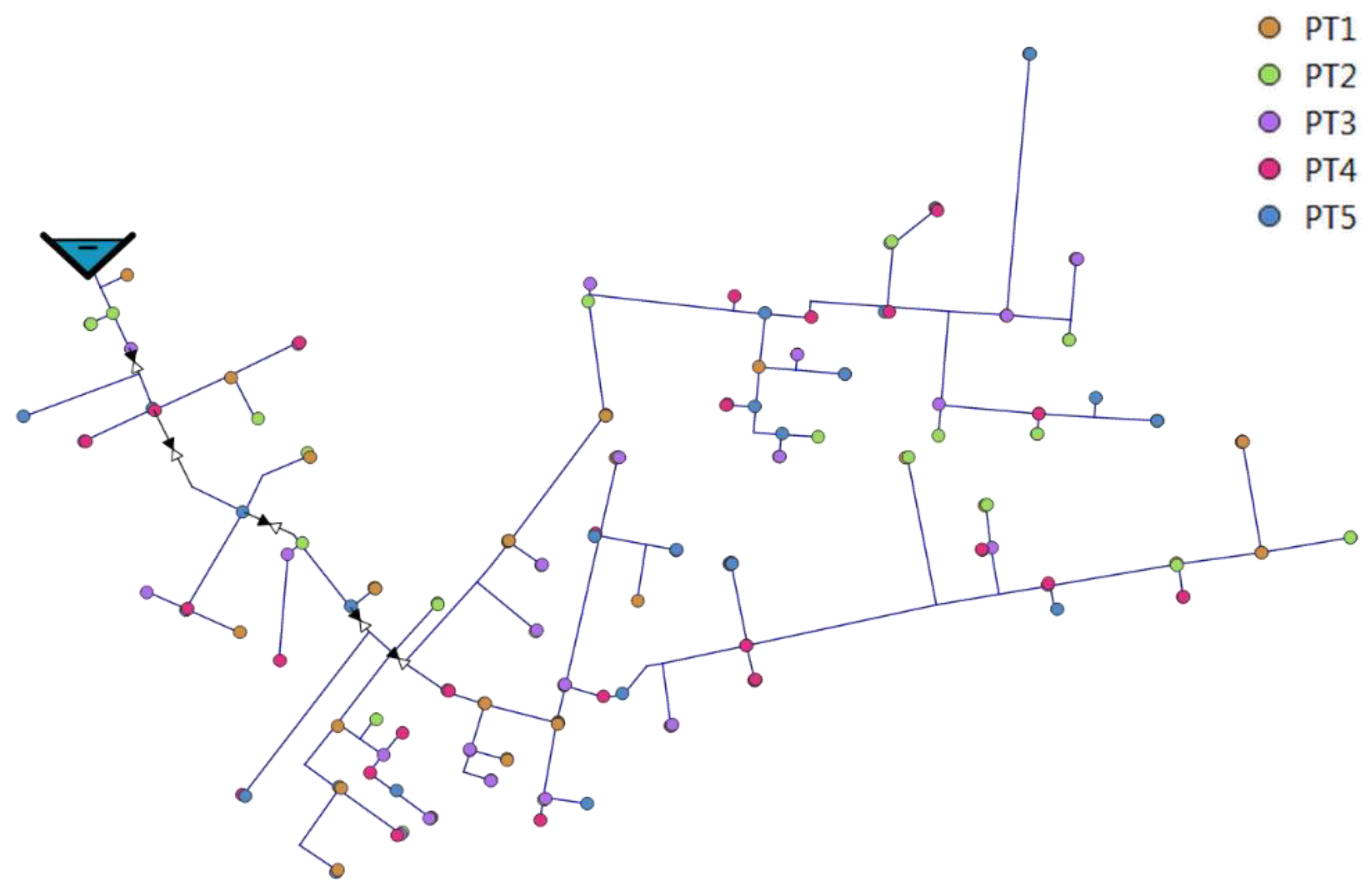
Data on the study area, both geographic and agronomic, are available at [14]. The gravity irrigation network is divided into five branches, nevertheless, for the research work, the branch called Yulchirón 2 will be used (Figure 1) with 171 hydrants represented by each node and an irrigation area of 23.38 ha. The network is supplied from the main reservoir by gravity. The elevation of the area ranks between 3210 and 3472 m. The total demand is 81.3 L/s. In Figure 1, the size of the hydrants is proportional to their demand.
2.2. Data and Materials
The meteorological information comprises a 22-year historical series (1990–2012) from two stations nearby the study area, obtained from the National Institute of Meteorology and Hydrology of Ecuador [15]. The rainfall station San Juan Chimborazo (code M0393, coordinates 1°37′35″ S and 78°47′0″ W, altitude 3220 m.a.s.l.), and the main meteorological station Querochaca UTA (code M0258, coordinates 1°22′2″ S and 78°36′20″ W, at an altitude of 2865 m) were determined.
2.3. Methodology
In order to achieve the research objective, a sequence of organised stages was established (Table 1).
2.3.1. Phase 1
For the agronomic design of the Yulchirón 2 branch, the meteorological annuals published by INAMHI were utilised [15] which provide a historical data series of 22 years. The Querochaca UTA weather station provided monthly average data on temperature (minimum and maximum), relative humidity and wind (Table 2). Based on the above information, annual average values were calculated (Table 3). The wind data were corrected with Equation (1) for a height of 2 m, according to the guidelines mentioned by FAO [11].
where: is the wind speed at 2 m above the surface [], corresponds to the wind speed measured at m above the surface [], and represents the measuring elevation above the ground surface [.
Whereas, the precipitation data obtained from the San Juan Chimborazo rainfall station were filled in with the method of proportionalities, which established the use of the average values of the data recorded during the period under analysis, therefore obtaining more reliable results. A reliable precipitation of 75% was considered and the USDA method was used to find the effective precipitation [19] (Table 3).
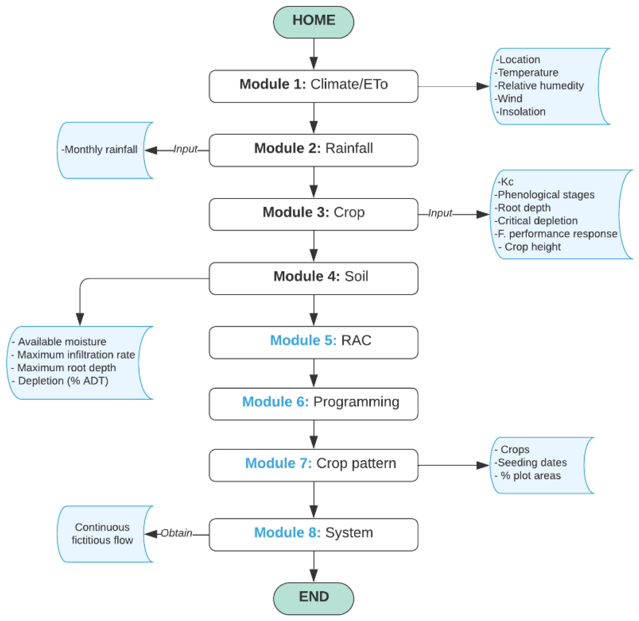
Data for crop types, crop coefficient (Kc) at different growth stages and soil data were provided by the Provincial Council of Chimborazo (CPCH, in its original Spanish) [14]. The other crop agronomic variables (growth stage, root depth, critical exhaustion, and yield response factor) were adopted from the help section of the CropWat 8.0 software [16], and following the guidelines of the FAO manual N°56 [11]. The continuous fictitious flow rate was determined using the FAO CropWat 8.0 software; in Figure 2, the procedure conducted is presented.
2.3.2. Phase 2
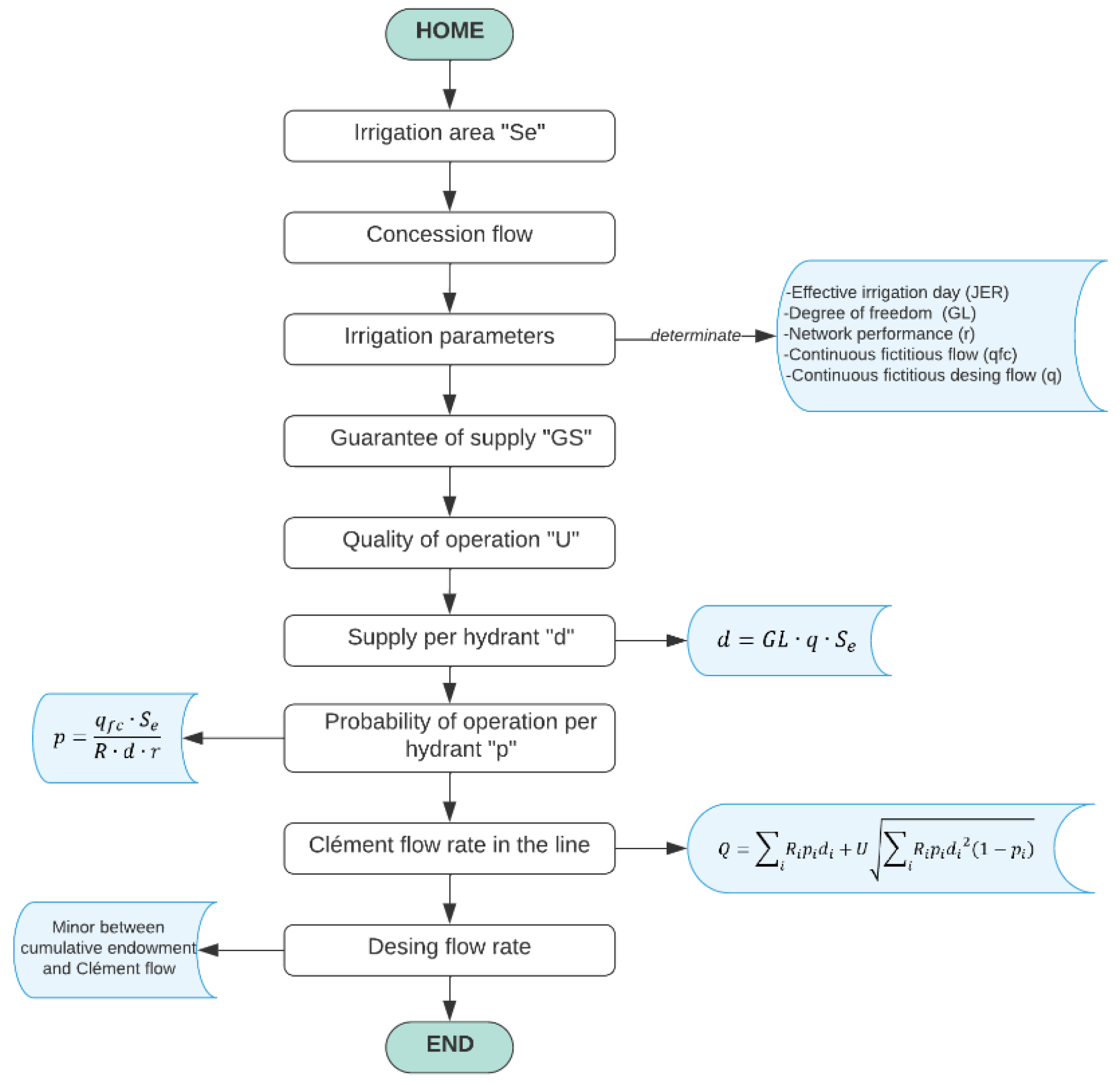
After phase 1, it is possible to compute the continuous fictitious flow, that is, the flow required to cover the water needs in the case that the area to be irrigated for a period of 24 h, usually expressed in l·s−1·ha−1. In other words, it is the volume needed to irrigate 1 ha of the crop equally distributed along the 24 h in a day. Other variables needed to fulfill the design of the network are the daily operating time or effective irrigation day (JER) and the degree of freedom (GL). The effective irrigation day is the time the network is actually available for irrigation throughout the day. The degree of freedom is defined as the relation between the flow rate actually assigned to the plot and the continuous fictitious flow. To determine the design demand flow rates for each line on the branch (Yulchirón 2, Figure 1), Clément’s first model was used [12] based on the guarantee of supply (GS), which was established according to the number of accumulated hydrants and therefore the quality of operation for the branch line; this method is used because it is the most commonly used due to its simple implementation worldwide [20]. In Figure 3, the procedure conducted is summarised. The calculations of the design flow rates on-demand made were checked in the GESTAR 2010 software [18].
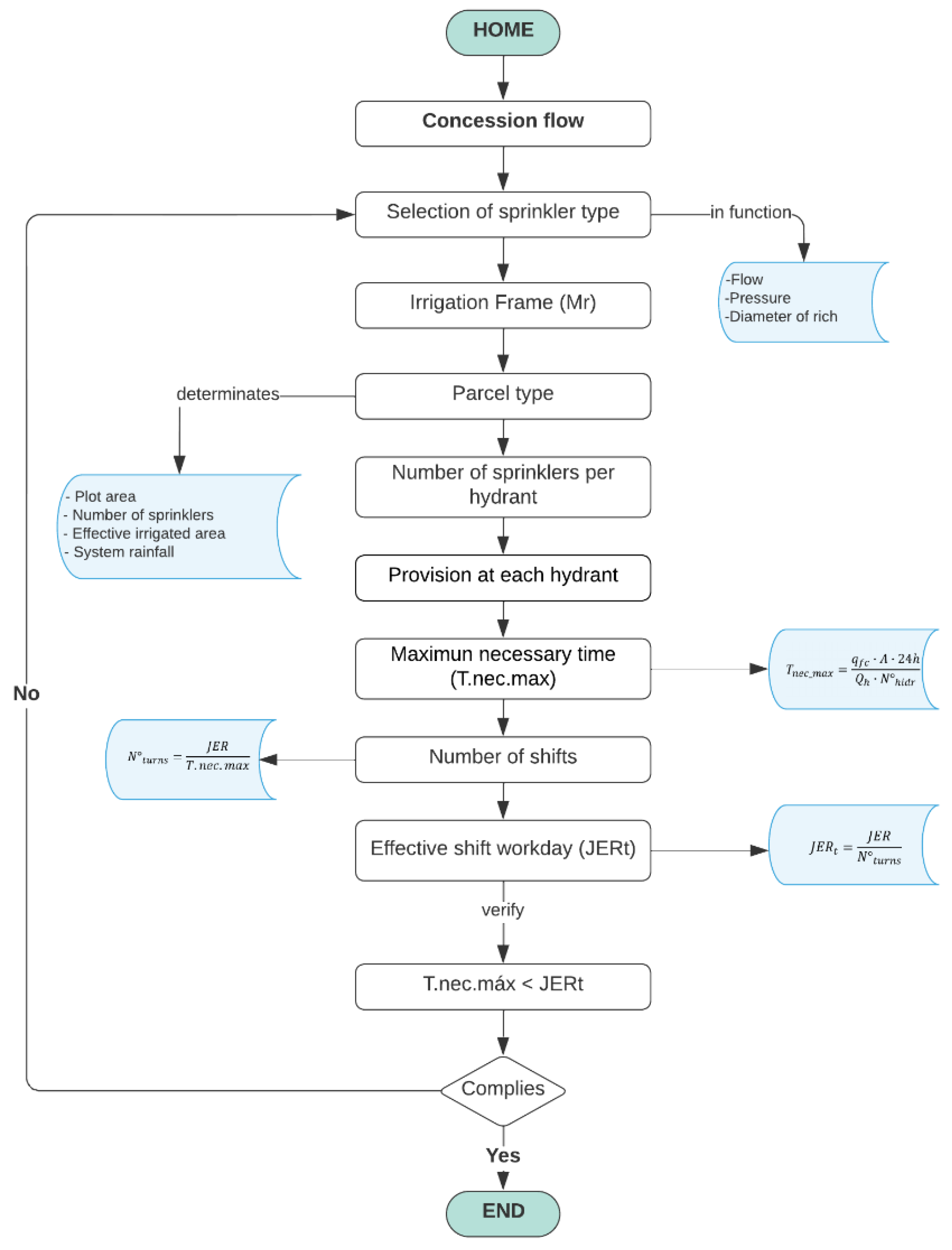
In order to determine the design flow rates at turns, the head flows of the branch under study were calculated (Yulchirón 2, Figure 1) through the design of the model plot Figure 4 The procedure developed is presented. Based on the concession flow rate, the project plots are standardised according to the standard plot (surface area of 1 ha). For this purpose, the “Wedge Drive Series 20” sprinkler was chosen with a pressure of 17.60 mwc, flow rate of 0.053 l/s and irrigation reach diameter of 18 m, data defined by the Senninger catalog. On the basis of these data, the number of emitters (sprinklers) in each plot and the hydrant endowments were defined based on the emitter coefficient, thus obtaining a maximum of 29 emitters and a minimum of 1 emitter corresponding to nodes 17 and 126 respectively.
The time required to open each hydrant was calculated () and eventually the maximum time required was chosen (), it was verified that the is less than the effective shift irrigation day “JERt” [13]. The design flow rates for each shift were determined from the sum of the open hydrants downstream of the corresponding shift. The diameters of all the lines were determined for each shift of the Yulchirón 2 branch [13]. The process was validated with EPANET 2.0 software [17].
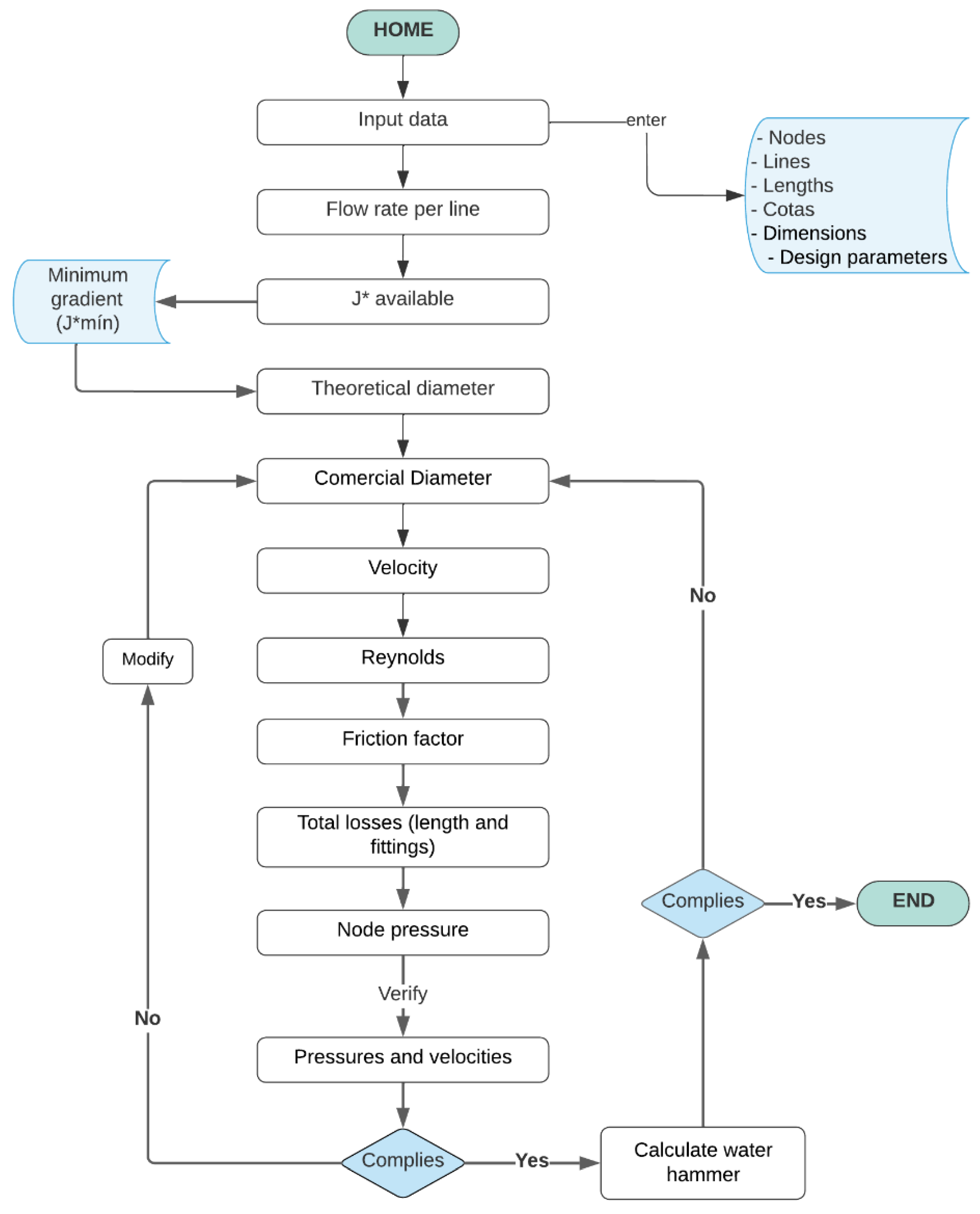
The hydraulic design was executed using the hydraulic gradient method for the two modes of operation of the study network (shifts and demand), the process of which is shown in Figure 5. All the pipes in the irrigation network were dimensioned according to the minimum or critical slope, which corresponds to the critical node. On this basis, the velocities in the network lines, the pressure at the nodes and the losses per length (Darcy-Weisbach equation) were determined, and the water hammer [21] was calculated to ensure that there is no damage to the system. According to Robalino and Lapo [22], the speed range for the design is between 0.5 m/s to 2.5 m/s, and the minimum design pressure in the network was given by the chosen sprinkler type. Verification of compliance with the design parameters in the study network was carried out using EPANET software [17].
2.3.3. Phase 3
For the modeling and simulation of the network, different scenarios were defined in order to represent emerging events that affect the operation of the irrigation system. Variations in critical variables such as demands and pressures in the network were considered in the two modes of operation.
2.3.4. On-Demand Mode of Operation
Scenario 1: It was assumed that the network configuration is modified understanding this as a group of hydrants operating at the same time [23]. In this context, it is known that the variation from one configuration to another is the main cause of disruptions in pressurized irrigation systems (Lamaddalena et al. [23]). Based on this premise, the guarantee of supply “GS” was modified from 90% to 99.5% in the network design, which directly influences the number of hydrants in operation and thus the flexibility of the system [24].
Scenario 2: It was assumed that there is a change in the initial crop pattern (main factor for estimating the amount of water [24]) and it was simulated and identified how these changes affect the demands and consignment pressures. It was considered that certain users decide to plant a new crop that demands a flow increase of 10% and 30%. For the simulation with the 10% increase in flow, the hydrants that would be affected were stochastically defined, initially considering 10% of the hydrants in the network, resulting in 18, with 30% of the hydrants in the network, 52, with 50% of the total hydrants, resulting in 86, and with 70% of the hydrants in the network, corresponding to 120 simulated hydrants. With the 30% increase in flow rate, we proceed to adopt the same percentage of hydrants in the network for the simulations.
2.3.5. Shift Operation Mode
Scenario 1: It was assumed that some users would not respect the assigned shift, so the Yulchirón 2 branch was analyzed under different service states. For this purpose, a shift in operation (shift two) was randomly established and simulated without any change, which is the initial state of the network. Then, the hydrants corresponding to different shifts were stochastically defined to be progressively opened in steps of 20%, up to a maximum of 50% of the hydrants.
Scenario 2: It was assumed that there is a change in the initial crop pattern (the main factor to estimate the amount of water [24]) was simulated and identified how these changes affect the demands and consignment pressures. It was considered that certain users of shift number 2, decide to plant a new crop that demands a flow increase of 10% and 30%. For the simulation with a flow increase of 10%, the hydrants that would be affected were defined stochastically, initially considering 10% of the hydrants in the network, which results in 4, with 30% of the hydrants in the network, there would be 11, with 50% of the total number of hydrants, there would be 17 and with 70% of the hydrants in the network, there would be 24 hydrants simulated. With the 30% increase in flow rate, the same percentage of hydrants in the network is adopted for the simulations.
Indicators allow performance to be assessed by means of mathematical formulations [9]. Resilience indices and their modifications have been applied to assess the reliability of a water network in the face of hydraulic variations [25]. The pipe resilience index was used in this research “PHRI” [10] and the availability index “Rsys” (Zhuang et al., 2012 in [5]).
PHRI developed by H. Liu et al. [10], is a method that combines pressure head and pipe length (relying on the hydraulic gradient of the pipe), which is linked to the difference in height at both ends of a pipe and the length of the pipe. The method states that more load will be obtained downstream, as long as the upstream pipes dissipate less energy. PHRI was calculated with Equation (2):
where: is the number of pipes in the water distribution system, correspond to the functions of the area are expressed in Equations (3) and (4), and is the length of the projection of the pipe, which is represented by Equation (5).
where: is the head at the downstream and upstream nodes respectively, for the pipeline , corresponds to the required system head.
On the other hand, the Rsys developed by [26], is a method that is based on terms of system availability, which is the amount of water that is supplied to the consuming nodes during unfavourable events in the system; this indicator can be calculated at the nodal level and at the system-wide level, it is expressed with the Equations (6) and (7).
where: is the availability of the system, correspond to the availability of the ith node, is the demand delivered to the ith node at time , is the demand required at the ith node at time , is the total period of time under the system’s unfavourable event, is the number of demand nodes.
The indicators described above assessed resilience on a range of 0 to 1, values close to 1 indicated that the system had high resilience, the opposite if the value was close to 0 [5,10]. Hence, the first indicator assessed the resilience of the whole system in terms of the pressure available at the nodes and the second in terms of the demand.
3. Results
The results obtained in the case study “San Francisco de Cunuguachay, Yulchirón 2 branch” are shown.
3.1. Continuous Notional Flow (Agronomic Design)
From the system provisioning module of the CropWat 8.0 software [16], the continuous fictitious flow rate was obtained, the value of which is 0.32 l/s/ha corresponding to the month of August, which requires a greater amount of water. That is to say, the value chosen was the maximum of all, in order to guarantee the necessary water in the period of the maximum irrigation campaign [27].
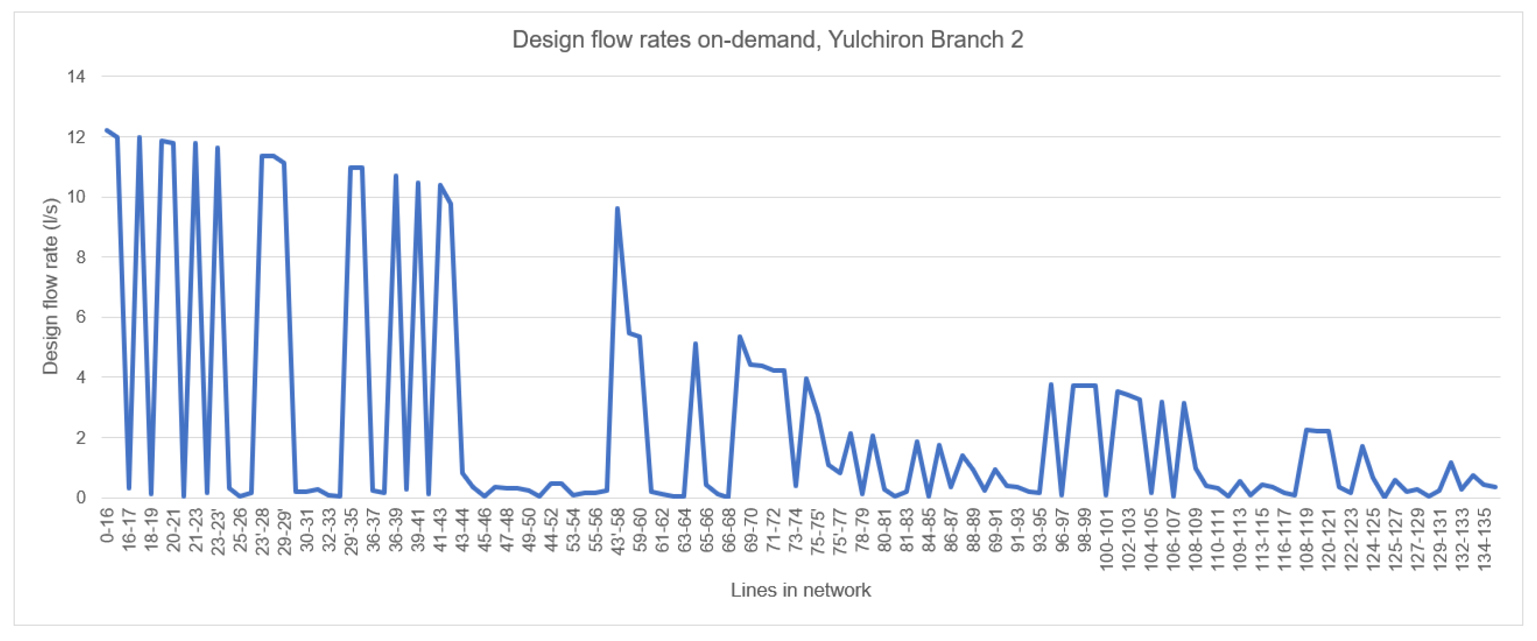
3.2. Design Flow On-Demand
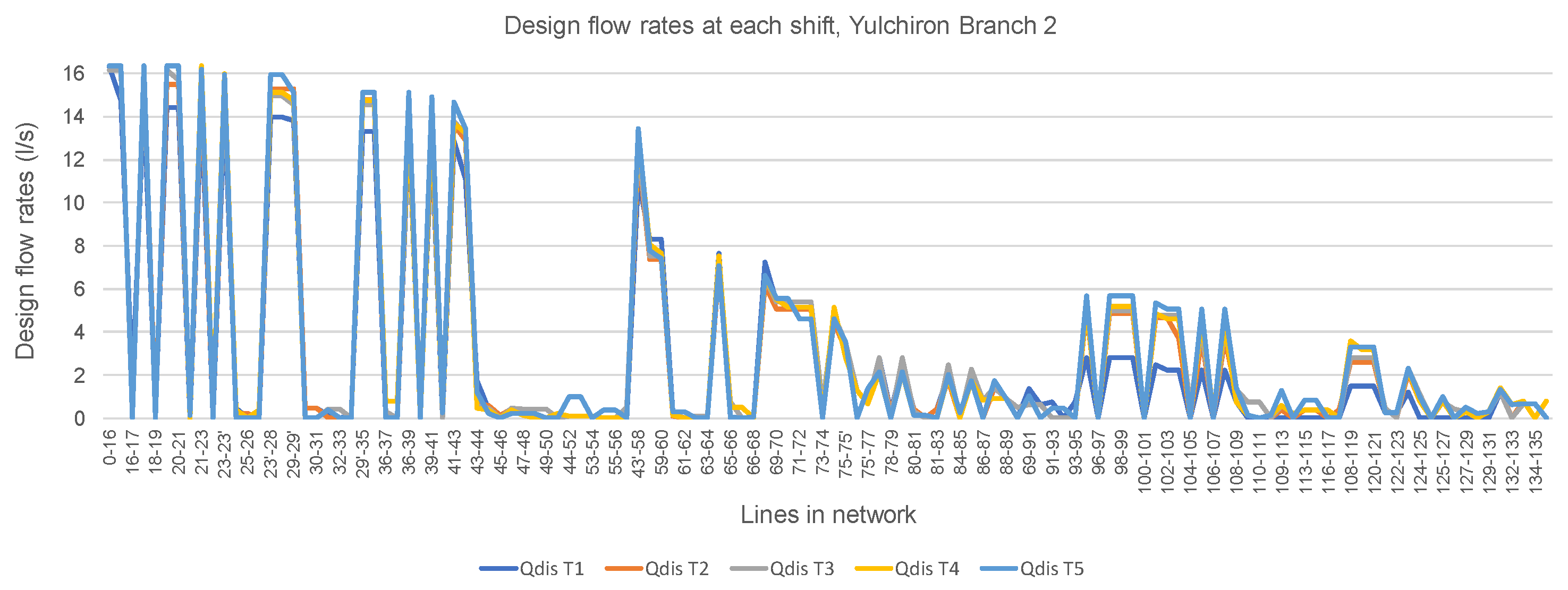
3.3. Shift Design Flow
3.4. Results of the Hydraulic Design of the Network Operating On-Demand and in Shifts
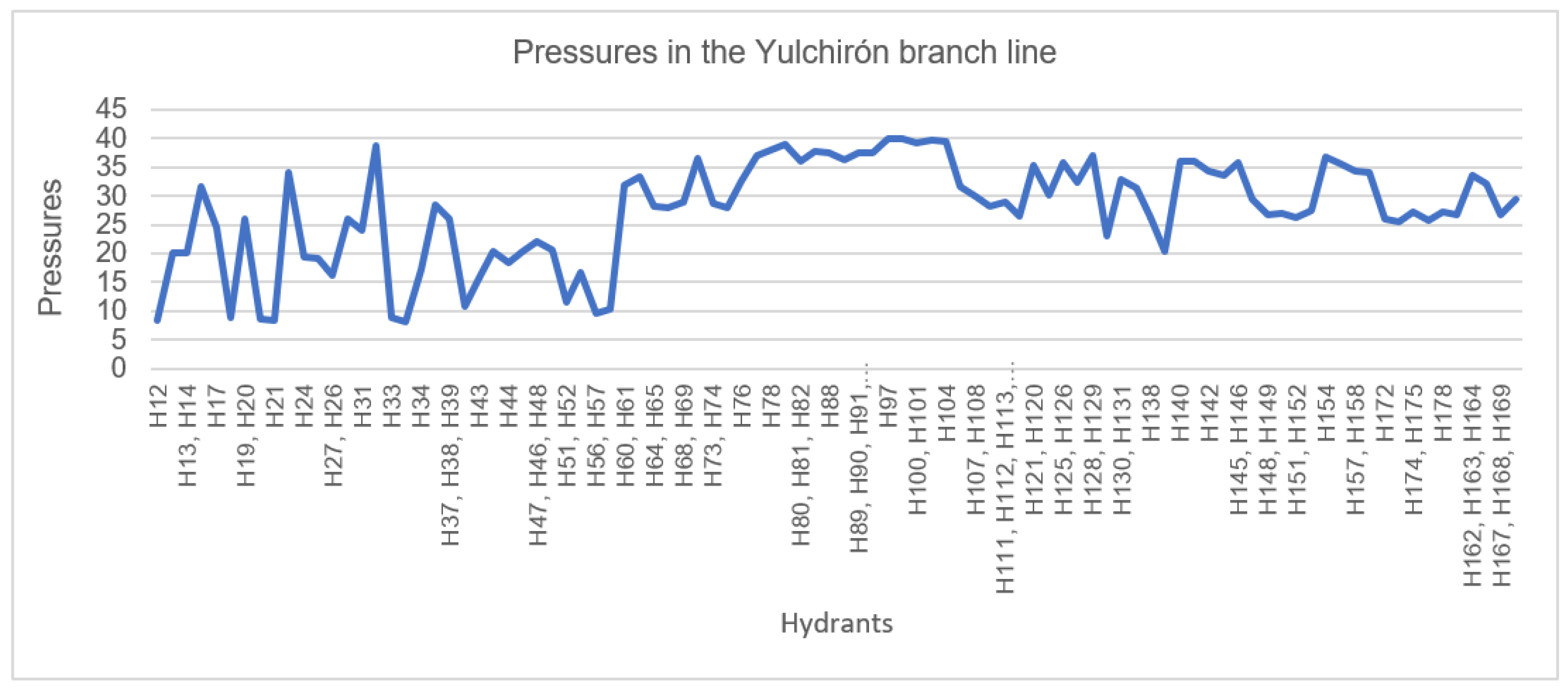
The pressure values of each hydrant obtained in the hydraulic design are shown in Figure 9, operating on-demand. It can be seen that the minimum pressure of the hydrants in the irrigation system is 8.19 mwc and the maximum pressure is 39.94 mwc. Therefore, complying with the minimum design pressure (set pressure) between 7 mwc and 50 mwc.
The range of design velocities on the Yulchirón 2 branch lines on-demand is between 0.10 m/s and 2.11 m/s. The sections of the network where a velocity of 0.1 m/s is obtained constitute 1.6%.
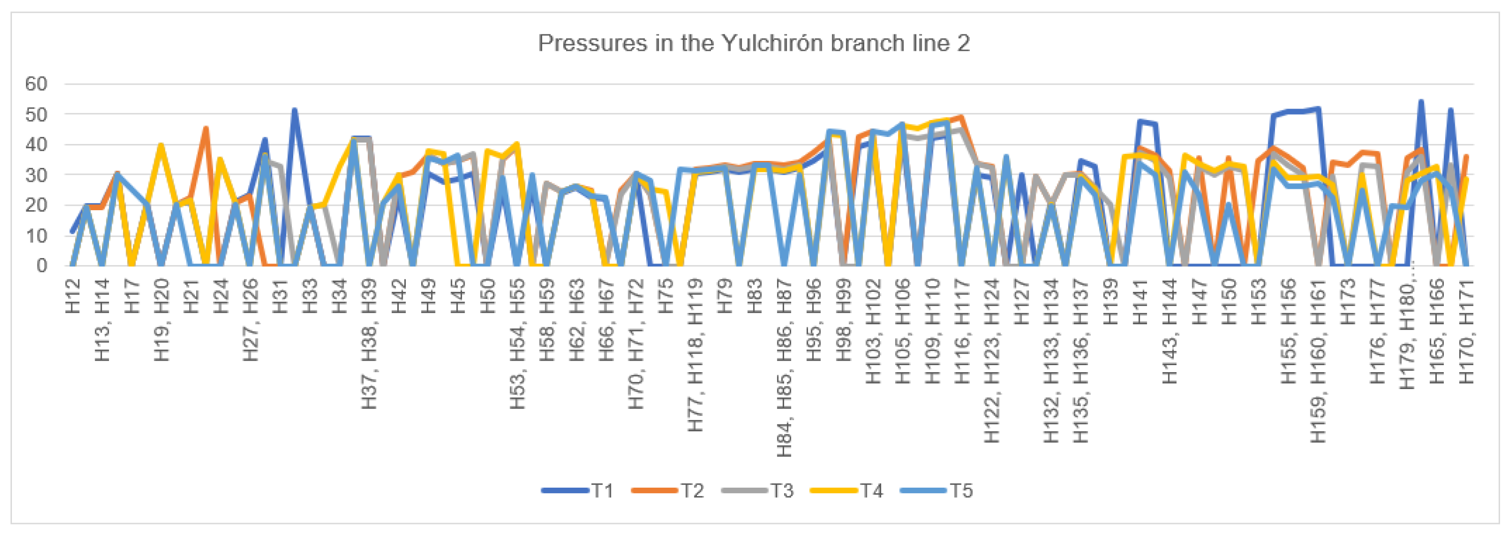
The operating hydrant pressures for each shift obtained from the hydraulic design are shown in Figure 10. The minimum pressures for shifts one to five are: 11.53, 19.43, 19.45, 19.37, 19.37 mwc and the corresponding pressures are: 54.12, 48.88, 44.89, 48.06, 47.09 mwc: 54.12, 48.88, 44.89, 48.06, 47.09 mwc, this at the nodes of known demand that are in the open shift. It can be seen that only shift one (T1) does not comply with the minimum design pressure (set pressure) of 17.6 mwc.
The minimum speeds on the lines of the Yulchirón 2 branch line are 0.39 m/s in shift one and 0.10 m/s in shifts two to five and the maximum speeds for shifts one to five are: 2.01, 1.99, 1.99, 1.99, 2.17, 2.02 m/s. The sections of the branch line where 0.1 m/s is obtained constitute 1.6%.
3.5. Results of the Calculation of the Indicators
The following section presents the results of the implementation of the indicators on the Yulchirón 2 branch in the two scenarios proposed for each mode of operation (demand and shifts).
3.5.1. Network Operating On-Demand, Scenario 1
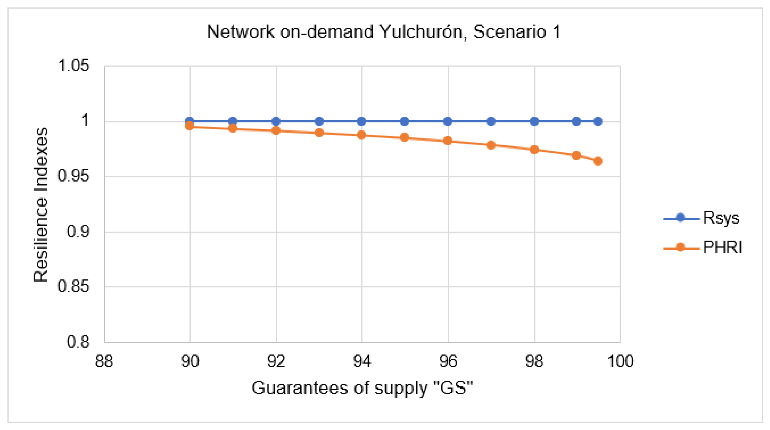
Table 4 shows the value of the resilience indices “Rsys” and “PHRI” in the Yulchirón 2 branch when the configuration of the hydrants is modified, by varying the supply guarantees “GS” from 90% (base case, which means, the Yulchirón 2 branch operating without any eventuality) to 99.5%. It is observed that the “Rsys” indicator is equal to 1 despite the increase in flow rate due to the increase in the number of hydrants in operation, when the GS is gradually increased.
In Figure 11 and as a consequence of the gradual variation of GS, it is observed that the trend of the values of the resilience indexes, “Rsys”remain constant; however, the PHRI indicator decreases as GS increases, due to the greater energy loss in the lines, in consequence, decreasing the pressures in the hydrants to a certain extent, as shown in Figure 12.
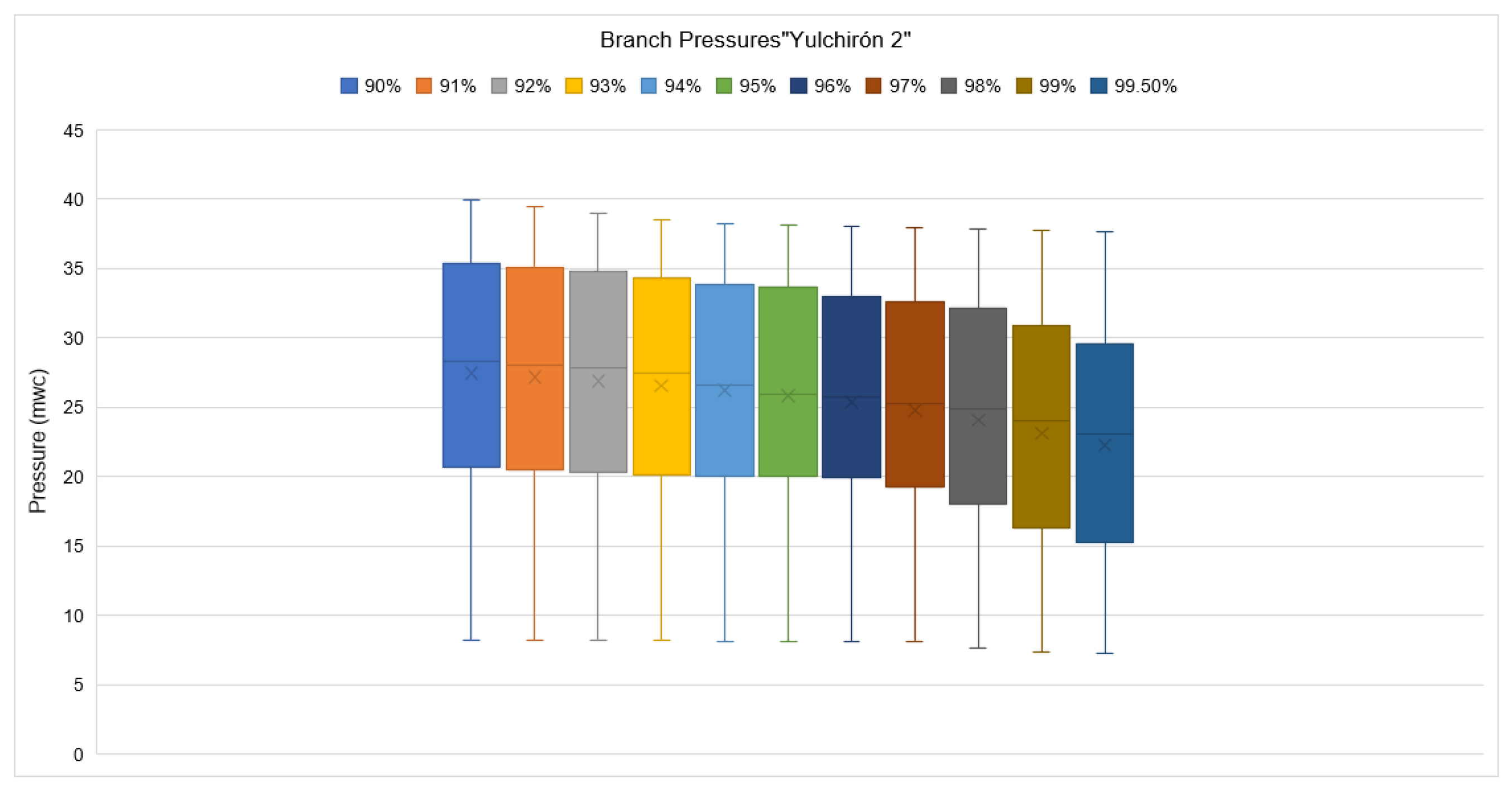
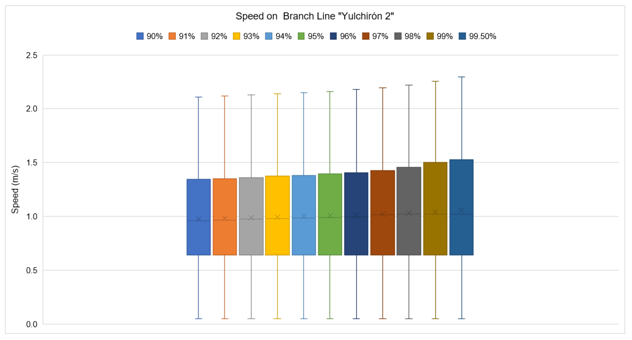
Figure 12 shows the variability of hydrant pressures in each case of scenario 1, the box and whisker plot corresponding to the GS equal to 90% is the initial state of the network or base case. The box and whisker plot with GS equal to 99.5% has the greatest symmetry and therefore has the least dispersion between pressure values. It has the lowest pressures with a minimum of 7.23 mwc and a maximum of 37.61 mwc. The highest dispersion of the pressure values is in the base case box plot with GS equal to 90%. In all the box and two-cot diagrams corresponding to the different GS, it is positively verified that the minimum pressure is higher than the design pressure (7 mwc).
Figure 13 shows the variability of the speed values on the network paths in each case of scenario 1. It is evident that the minimum speed is 0.10 m/s in all graphs, which represents 1.6% of the lines. The maximum speeds increase in each graph from 2.11 m/s (GS = 90%) to 2.29 m/s (GS = 99.5%). The lowest dispersion of the velocity values is in the box and whisker plots GS equal to 90% and 91% as they have the same symmetry; however, the largest dispersion of velocity values is in the box plot with GS equal to 99.5% as it is the most asymmetric and has the widest range.
3.5.2. Network Operating On-Demand, Scenario 2
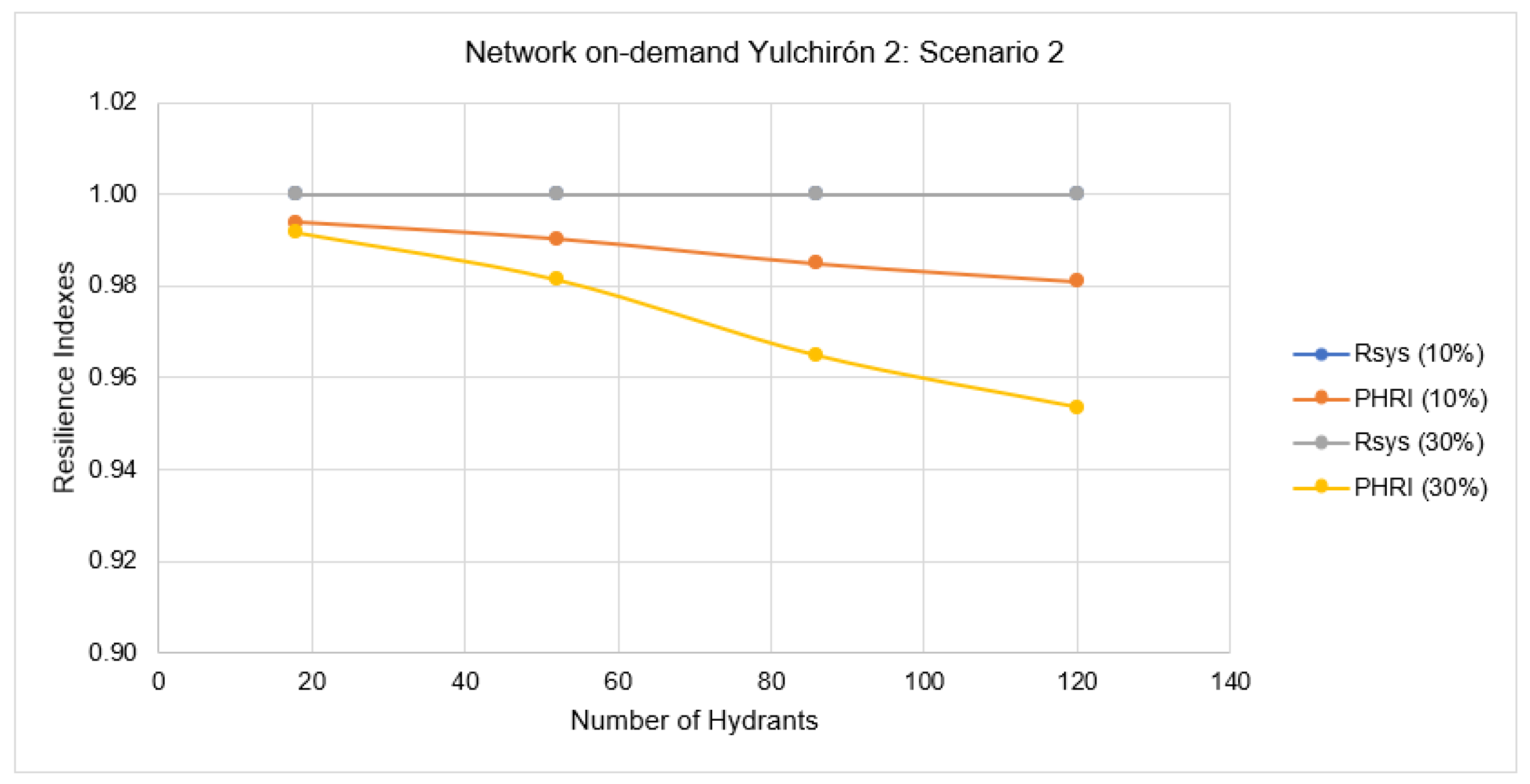
Table 5 shows the value of the resilience indices “Rsys” and “PHRI” in the Yulchirón 2 branch when there is a change in the crop pattern, at the moment when the demand is increased by 10% and 30% respectively, for different hydrants that were defined as explained in the methodology section, specifically in “simulation scenarios”. It is observed that the Rsys is equal to 1, which indicates that the branch has the maximum resilience at the demand level. The maximum PHRI value is 0.994 when the flow is increased by 10% at 18 hydrants and the minimum PHRI value is 0.954 when the flow is increased by 30% at 120 hydrants. In both cases good pressure resilience is evident.
Figure 14 visualises the trend of the resilience indices, the Rsys index remains constant despite the increase in flow, while the PHRI index decreases as a function of the variation in flow. The values of the resulting indices (PHRI and Rsys) range from 0 to 1, he closer to 1 indicating greater resilience. In this case, it is clearly evident that the network has good resilience in terms of both pressures and demands, despite the eventuality to which it was exposed.
The variability of the hydrant pressures when considering a 10% increase in flow rate shows that the minimum pressure is higher than the design pressure (7 mwc); however, when a 30% increase in flow rate was considered, the minimum pressure was not met in hydrants 52H (30%) and 86H (30%), obtaining a minimum pressure of 5.90 mwc and 4.63 mwc, respectively.
3.5.3. Network Operating in Shifts, Scenario 1
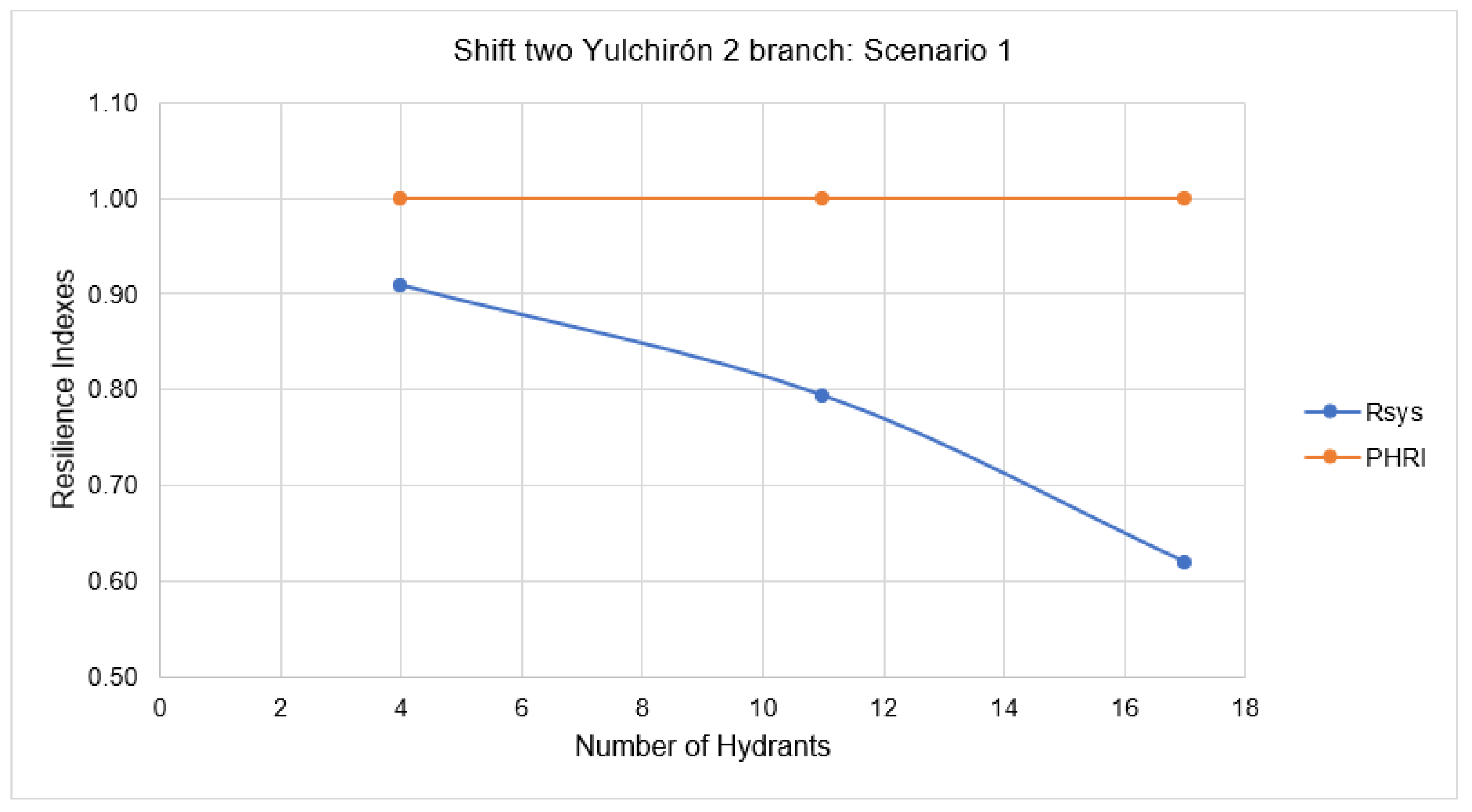
Table 6 presents the value of the resilience indices “Rsys” and “PHRI” in the Yulchirón 2 branch, turn two (T2), in which the increase in the number of open hydrants (column two, users who did not respect their turn) was considered. The minimum value of the Rsys index is 0.62 (lower resilience) and the maximum is 0.91 (higher resilience). The PHRI in all scenarios is 1, as a result, the maximum resilience is at the level of pressures.
Figure 15 illustrates the trend in the resilience indices. In this case, as the Rsys index decreases, the PHRI index remains constant. It is clearly evident that when there is a higher number of hydrants operating in turn two the resilience of the network drops to 0.62.
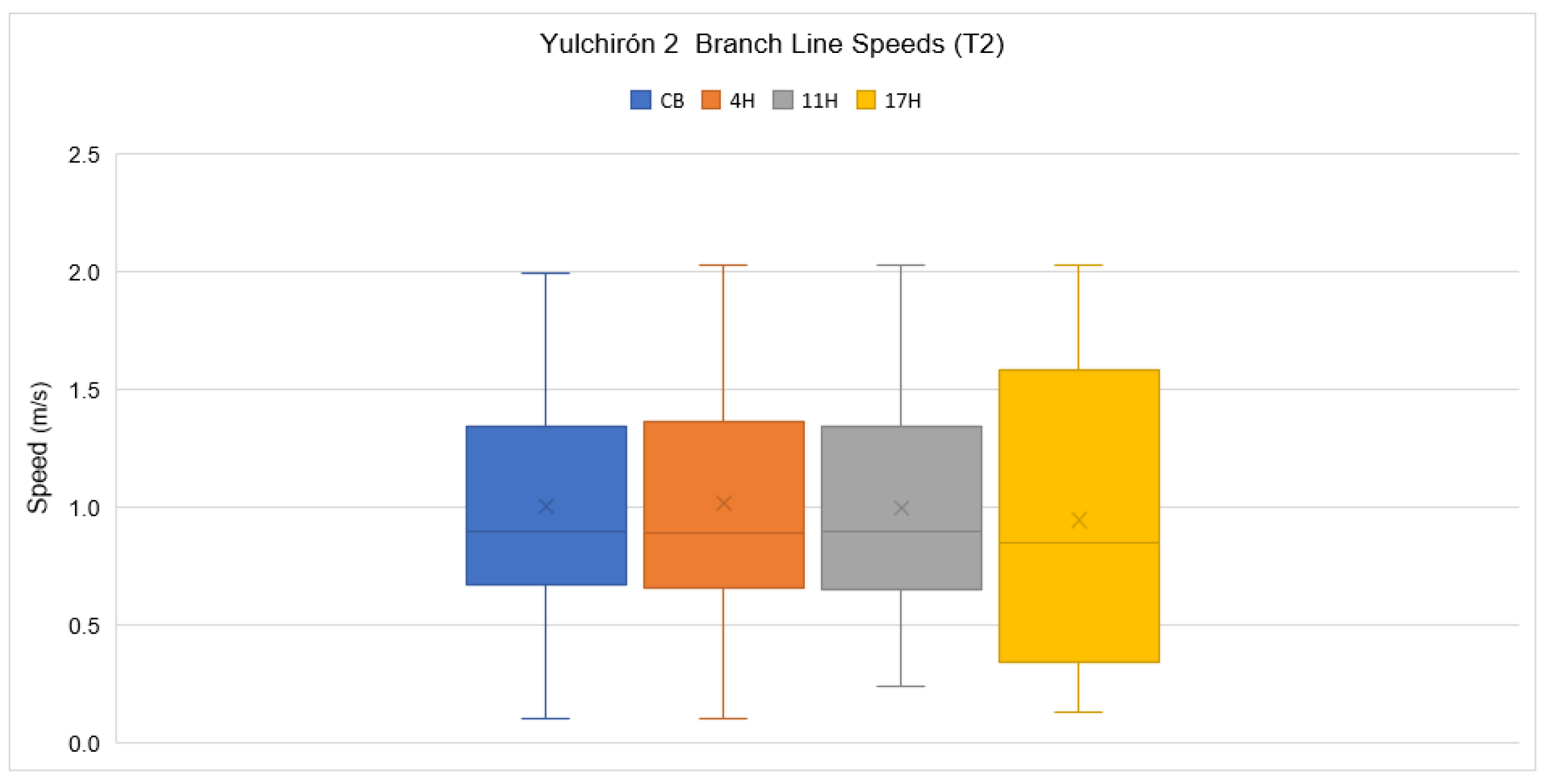
Figure 16 illustrates the variability of the line velocity values in each case of Scenario 1 in shifts. The minimum velocity is 0.10 m/s (representing 1.6% of the lines) because in the shift design the diameter chosen for these lines must allow the flow of all other shifts to pass through. The maximum velocity in the CB is 1.99 m/s in the rest of the graphs is 2.03 m/s, therefore, they comply with the maximum design velocity 2.5 m/s. The lowest dispersion of the values of the velocity obviating the CB box diagram is given in the 11H box diagram as it has a range of 1.79, it also presents a positive asymmetry as the lower part of the box is lower than the upper part. On the other hand, the greatest dispersion of data is found in box plot 4H, which has a range of 1.93 and a positive asymmetry.
3.5.4. Network Operating in Shifts, Scenario 2
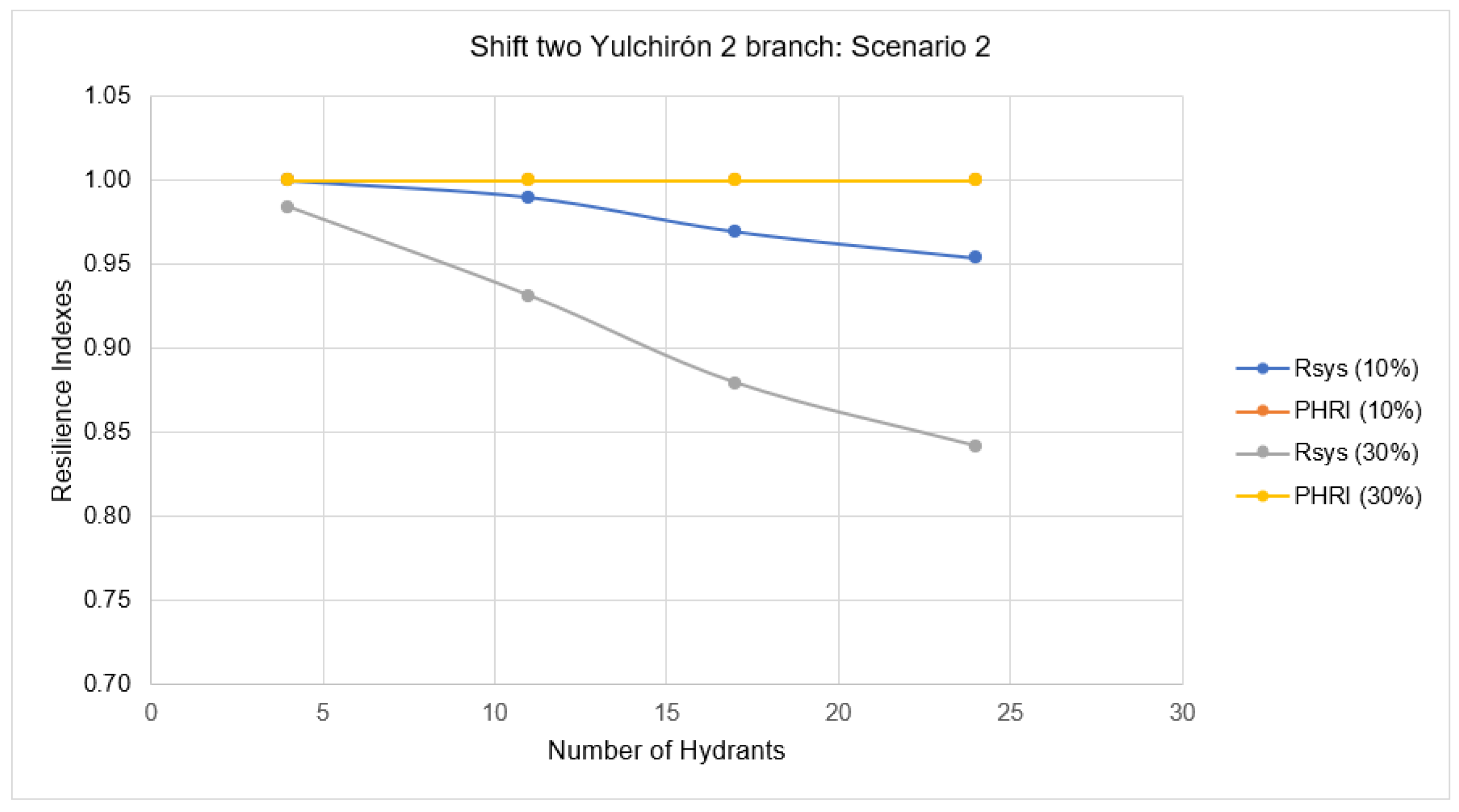
Table 7 presents the value of the resilience indices “Rsys” and “PHRI” in the Yulchirón branch 2 turn two (T2), in which a change in the crop pattern was considered, therefore increasing the demand by 10% and 30% respectively, this for different hydrants that were defined as explained in the methodology section, specifically in “simulation scenarios”. It is observed that when the flow rate was increased by 10% in 4 randomly chosen T2 hydrants, the Rsys is 1, which indicates that for this eventuality the system is resilient; this is because the flow that is required despite the increase can be delivered by the branch, as T2 has a flow slack of 0.36 l/s to reach the design flow (16.5 l/s). On the other hand, when there is a 30% increase in flow in 24 hydrants in T2, the lowest Rsys is 0.84, which indicates that the resilience has decreased due to the fact that more flow is required than can be delivered. The PHRI is equal to 1 in all cases regardless of the increase in flow, hence establishing that the resilience at pressure level is excellent in T2 of the Yulchirón 2 branch.
Figure 17 shows the trend of the resilience indices, as the Rsys index decreases the PHRI index remains constant when the flow is increased from 10% to 30%. It is clearly observed that when more demand is required in the system, the system loses resilience in terms of water availability.
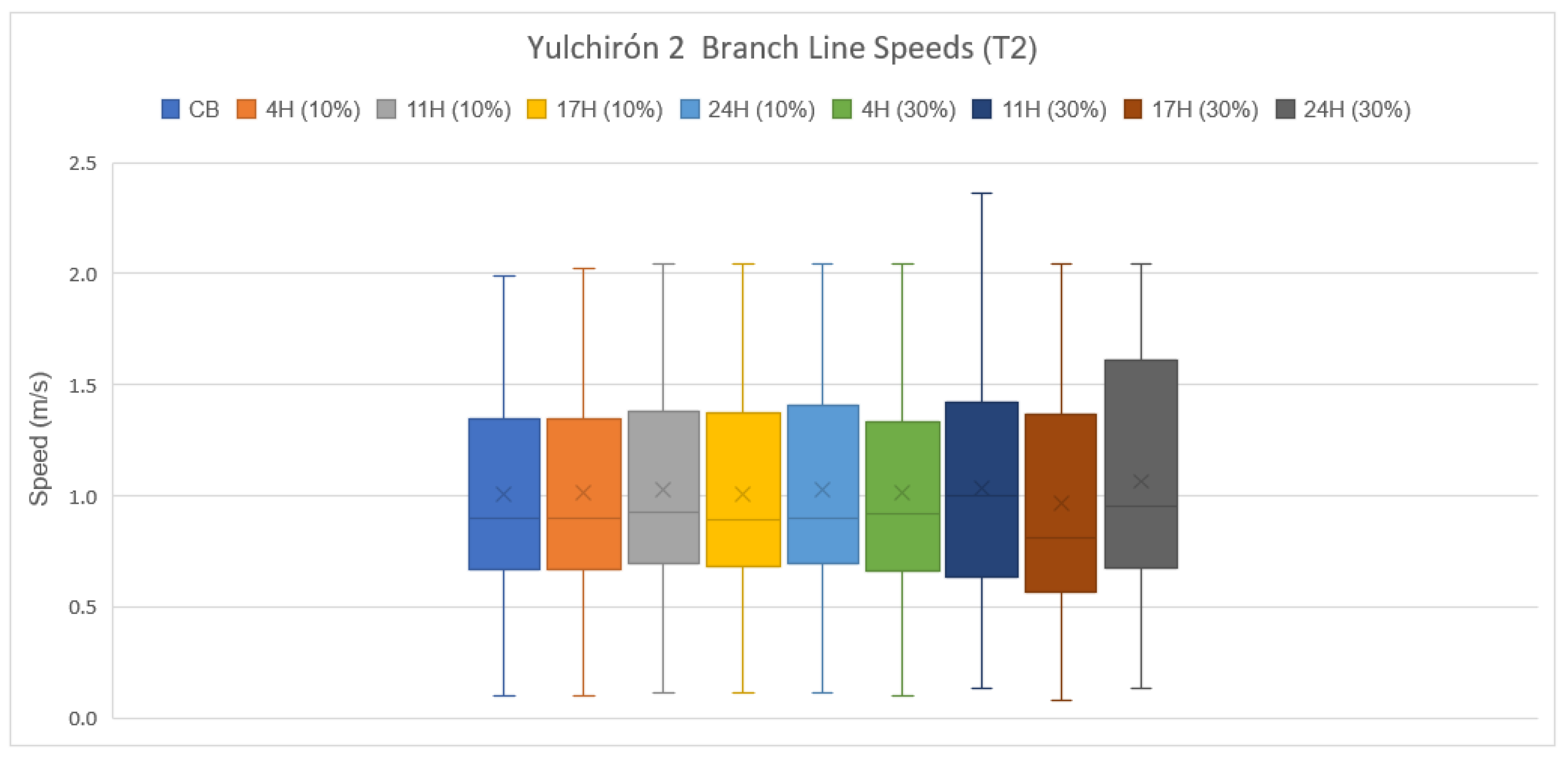
Figure 18 illustrates the variability of the line velocity values in each case of scenario 2. The minimum velocity is 0.10 m/s (representing 1.6% of the lines) in all cases because in the shift design the diameter chosen for these lines must allow the flow of all other shifts to pass through. The maximum velocity when considering the 10% increase in flow is 2.04 m/s and is given in the box and whisker diagrams 17H (10%) and 24H (10%). At 30% flow increase the maximum velocity occurs in the box and whisker diagram 11H (30%) at 2.36 m/s. Therefore, the maximum di-brain velocity of 2.5 m/s is fulfilled. It is observed that all box plots show a positive asymmetry indicating that the values above the median are further apart. The smallest dispersion of the velocity values without considering the CB box plot originates in the 4H box and whisker plot (10%) as it presents the smallest range equal to 1.92. The highest dispersion is observed in the box diagram 11H (30%) which presents the highest range with a value equal to 2.23.
4. Discussion of Results
In the research, the indicators were implemented in the case study which was designed with parameters such as degree of freedom “GL” of 1.5, effective irrigation day “JER” 16 h, continuous notional flow rate “qfic” of 0.32 l/s/ha, and following the design basis provided in the report granted by the Provincial Council of Chimborazo (CPCH). In this regard, design diameters were obtained that were very similar to the design of the CPCH; this design will be the base scenario (base case or initial state) for the generation of scenarios. In the CB box diagram it is evident that in certain lines the minimum speed is not complied with, however the pressures are complied with in all hydrants, as they are within the design range of each mode of operation.
It is also evident in the design on-demand that as the flow rate increases due to the eventualities encountered, there is more energy dissipation in the lines as an additional 8% and 2% of the flow rate is circulating Table 4 and Table 5 respectively, which causes the velocities in the pipelines to increase, resulting in lower pressures at the hydrants or nodes of known demand; this situation is reflected in the PHRI indicator, see Figure 11 and Figure 14 [10]
In the shift design, the demand resilience indicator Rsys decreases as more hydrant demand availability is required due to the scenarios encountered (Figure 15 and Figure 17); this situation leads to a lower resilience as the flow delivered in each eventuality will be a maximum of the concession flow (16.5 l/s), which is lower than the required flow rate. Table 6 and Table 7 [26].
At the same time, the resilience at the pressure level, evaluated with the PHRI, is constant in all the scenarios, since the maximum flow that can be delivered is the concession flow at the headworks level, which is greater than the design flow for turn 2 (T2, 16. 14 l/s) with which the lines were sized. Therefore, with a flow increase of 0.36 l/s there is no considerable energy dissipation since the designed diameters do not cause a significant increase in velocities (energy loss), this reflects the fact that the network scenarios analyzed can withstand abrupt pressure changes at their consumption nodes [10].
From scenario 1 generated for the network operating at demand, it can be observed that the box-and-whisker diagram for pressures (Figure 12) shows greater symmetry, evidencing less dispersion in the pressure values at the network consumption nodes. Box plot generated for a GS equal to 99.5, which is not indicative of better resilience at the level of pressures since the PHRI index for this scenario presents the lowest resilience with a value of 0.964 (Figure 11); this is because the PHRI indicator is based on the hydraulic gradient, indicating that if upstream pipes dissipate less energy, downstream pipes will achieve higher pressures or load [10], thereby establishing that higher pressures in a water network allow for better handling of disruptions.
Finally, these resilience indicators “Rsys” and “PHRI” when evaluated on a range of 0 to 1, as well as Todini’s resilience indicator, the researchers Saldarriaga et al. [29] quoted in [30] established that the limit value for assessing resilience is equal to 0.5, i.e., if a network has an index lower than 0.5, the network is considered vulnerable. In this context, according to the calculations of the indicators in the different scenarios in the two modes of operation of the network presented in Table 4, Table 5, Table 6 and Table 7. The values of the indicators are above the aforementioned limit, which establishes that despite the disruptions to which the network was subjected, it has a good resilience.
5. Conclusions
In this paper, an irrigation network operated in an on-demand basis was compared to an alternative operation based on a rotation system in different turns. Two resilience indicators (PHRI and Rsys) were used to quantify the comparison. As a result, some interesting conclusions were achieved.
- Irrigation networks operated on demand work in a more flexible way. Hence On demand operated networks do not have disadvantages when water demands are modified. The demand indicator Rsys reach optimal values in the different scenarios proposed for this research.
- Irrigation networks operated in rotation using shifts have a very low flexibility. Whenever there is a disruptive event requiring an increase in flow rate, problems associated with demands arise; this fact is shown by the value of the Rsys indicator, taking much smaller values with respect to those in an on-demand operation.
- The resilience indicators based on demand (Rsys) and on pressure (PHRI) allow to assessing the resilience of both operation modes. The pressure resilience indicator (PHRI)is ideal for assessing an irrigation network operated on demand since the hydraulic behaviour of the network is not affected by changes in operation.
- The demand resilience indicator (Rsys) makes evident the effect that changes in demands have on the consumption nodes of the network.
In conclusion, this research shows the importance of using these two resilience indicators to evaluate how an irrigation network responds to changes in demand or operation mode; this way it is possible planning and managing the networks before they are in operation, facilitating the decisions taking by the project manager.
Author Contributions
All authors contributed extensively to the work presented in this paper. Conceptualization, C.M.L.P. and H.B.M.; Data curation, V.A.B.O.; Investigation, C.M.L.P., V.A.B.O. and H.B.M.; Methodology, C.M.L.P., V.A.B.O. and H.B.M.; Supervision, H.B.M.; Writing—original draft, C.M.L.P. and H.B.M.; Writing—review and editing, V.A.B.O., F.J.M.-S. and H.B.M. All authors have read and agreed to the published version of the manuscript.
Funding
Universidad Técnica Particular de Loja (Ecuador).
Institutional Review Board Statement
Not applicable.
Informed Consent Statement
Not applicable.
Data Availability Statement
Not applicable.
Conflicts of Interest
The authors declare no conflict of interest.
References
- FAO. Water for Sustainable Food and Agriculture: A Report Produced for the G20 Presidency of Germany; Food and Agriculture Organization of the United Nations: Roma, Italy, 2017. [Google Scholar]
- Playán, E.; Mateos, L. Modernization and optimization of irrigation systems to increase water productivity. Agric. Water Manag. 2006, 80, 110–116. [Google Scholar] [CrossRef]
- D’Urso, G.; Richter, K.; Calera, A.; Osann, M.A.; Escadafal, R.; Garatuza-Pajan, J.; Hanich, L.; Perdigão, A.; Tapia, J.B.; Vuolo, F. Earth Observation products for operational irrigation management in the context of the PLEIADeS project. Agric. Water Manag. 2010, 98, 271–282. [Google Scholar] [CrossRef]
- Ministerio de Agricultura, Ganadería, Acuacultura y Pesca—MAGAP. La Política Agropecuaria Ecuatoriana: Hacia el Desarrollo Territorial Rural Sostenible: 2015–2025; MAGAP: Quito, Ecuador, 2016.
- Shin, S.; Lee, S.; Judi, D.R.; Parvania, M.; Goharian, E.; McPherson, T.; Burian, S.J. A systematic review of quantitative resilience measures for water infrastructure systems. Water 2018, 10, 164. [Google Scholar] [CrossRef]
- Hosseini, S.; Barker, K.; Ramirez-Marquez, J.E. A review of definitions and measures of system resilience. Reliab. Eng. Syst. Saf. 2016, 145, 47–61. [Google Scholar] [CrossRef]
- Liu, D.; Chen, X.; Nakato, T. Resilience Assessment of Water Resources System. Water Resour. Manag. 2012, 26, 3743–3755. [Google Scholar] [CrossRef]
- Butler, D.; Farmani, R.; Fu, G.; Ward, S.; Diao, K.; Astaraie-Imani, M. A new approach to urban water management: Safe and sure. Procedia Eng. 2014, 89, 347–354. [Google Scholar] [CrossRef]
- Ayala Cabrera, D.; Piller, O.; Herrera, M.; Gilbert, D.; Deuerlein, J. Absorptive resilience phase assessment based on criticality performance indicators for water distribution networks. J. Water Resour. Plan. Manag. 2019, 145, 04019037. [Google Scholar] [CrossRef]
- Liu, H.; Savić, D.A.; Kapelan, Z.; Creaco, E.; Yuan, Y. Reliability surrogate measures for water distribution system design: Comparative analysis. J. Water Resour. Plan. Manag. 2017, 143, 1–14. [Google Scholar] [CrossRef]
- Smith, M.; Allen, R.; Pereira, L. Revised FAO Methodology for Crop-Water Requirements. 1998. Available online: https://www.osti.gov/etdeweb/servlets/purl/676839 (accessed on 30 May 2022).
- Lamaddalena, N.; Sagardoy, J. Performance Analysis of On-Demand Pressurized Irrigation Systems; FAO—CIHEAM Bari Institute: Rome, Italy, 2000. [Google Scholar]
- Lapo, P.C.M.; Pérez-García, R.; Aliod-Sebastián, R.; Martínez-Solano, F.J. Optimal design of irrigation network shifts and characterization of their flexibility. Tecnol. Cienc. Agua 2020, 11, 266–314. [Google Scholar]
- Consejo Provincial De Chimborazo. Estudio de Factibilidad y Diseño Definitivo para el Sistema de Riego de la Comunidad San Francisco de Cunuguachay—Vertiente Chinigua; CPCH: Chimborazo, Ecuador, 2010.
- Instituto Nacional de Meteorología e Hidrología (INAMHI). Anuarios Metereológicos; INAMHI: Quito, Ecuador, 2012.
- Smith, M. CROPWAT: A computer program for irrigation planning and management. FAO Irrig. Drain. 1996, 46, 127. [Google Scholar]
- Rossman, L.A. EPANET 2 Users Manual; EPA/600/R-00/057; U.S. Environmental Protection Agency: Cincinnati, OH, USA, 2000.
- Estrada, C.; González, C.; Aliod, R.; Paño, J. Improved pressurized pipe network hydraulic solver for applications in irrigation systems. J. Irrig. Drain. Eng. 2009, 135, 421–430. [Google Scholar] [CrossRef]
- Carrazón Alocén, J. Manual Práctico para el Diseño de Sistemas de Minirriego; FAO: Roma, Italy, 2007. [Google Scholar]
- Pérez-Sánchez, M.; Carrero, L.M.; Sánchez-Romero, F.J.; López-Jiménez, A. Comparison between Clément’s First Formula and other statistical distributions in a real irrigation network. Irrig. Drain. 2018, 67, 429–440. [Google Scholar] [CrossRef]
- Benavides Muñoz, H.; Cueva Torres, J. Laboratorio virtual para el cálculo de fenómenos transitorios en redes de agua a presión por el método de las características. AXIOMA 2017, 17, 28–44. [Google Scholar]
- Robalino Quizhpe, B.G.; Lapo Pauta, C.M. Caracterización de Parámetros para el Diseño Hidráulico de Redes de Riego a Presión y Redes de Abastecimiento, con Empleo de Software de Aplicación. Bachelor’s Thesis, Universidad Técnica Particular de Loja, Loja, Ecuador, 2018. [Google Scholar]
- Derardja, B.; Lamaddalena, N.; Fratino, U. Perturbation indicators for on-demand pressurized irrigation systems. Water 2019, 11, 558. [Google Scholar] [CrossRef]
- Granados, A. Criterios para el Dimensionamiento de Redes de Riego Robustas Frente a Cambios en la Alternativa de Cultivos; UPM: Madrid, Spain, 2013. [Google Scholar]
- Moosavian, N.; Lence, B.J. Flow-Uniformity Index for Reliable-Based Optimal Design of Water-Distribution Networks. J. Water Resour. Plan. Manag. 2020, 146, 04020005. [Google Scholar] [CrossRef]
- Zhuang, B.; Lansey, K.; Kang, D. Resilience/availability analysis of municipal water distribution system incorporating adaptive pump operation. J. Hydraul. Eng. 2013, 139, 527–537. [Google Scholar] [CrossRef]
- Lapo Pauta, C.M. Diseño Óptimo de Redes de Riego a Presión Para su Explotación a Turnos. Ph.D. Thesis, Universidad Politécnica de Valencia, Valencia, Spain, 2019. Available online: https://riunet.upv.es/handle/10251/130210 (accessed on 25 September 2019).
- Mena Trelles, Y.C.; Lapo Pauta, C.M. Herramienta Virtual para Cálculo de Caudales Circulantes en Redes de Riego a Presión y su Aplicación en el Diseño. Bachelor’s Thesis, Universidad Técnica Particular de Loja, Loja, Ecuador, 2019. [Google Scholar]
- Saldarriaga, J.; Páez, D.; Salcedo, C.; Cuero, P.; López, L.L.; León, N.; Celeita, D. A Direct Approach for the Near-Optimal Design of Water Distribution Networks Based on Power Use. Water 2020, 12, 1037. [Google Scholar] [CrossRef] [Green Version]
- Cambisaca Díaz, D.A. Valoración de Déficit de Energía con Varias Casuísticas en una red de Riego, con uso de Software de Aplicación; Universidad Técnica Particular de Loja: Loja, Ecuador, 2016. [Google Scholar]
Figure 1.
Planimetry of the network San Francisco de Cunuguachay.

Figure 2.
Flowchart of the CropWat 8.0 software modules.

Figure 3.
Flowchart of the design flow on-demand procedure.

Figure 4.
Flowchart of the design flow rate procedure for shift design flows.

Figure 5.
Flowchart of the hydraulic gradient method.

Figure 6.
Results of design flows on–demand, Yulchirón branch 2.

Figure 7.
Results of the design flow rates at turns, in the Yulchirón 2 branch.

Figure 8.
Description of the shifts in the Yulchiron 2 network.

Figure 9.
Pressure results, on the Yulchirón 2 branch operating at demand.

Figure 10.
Pressure results, on the Yulchirón 2 branch operating in shifts.

Figure 11.
“Rsys” and “PHRI” results, in scenario 1 on-demand.

Figure 12.
Yulchirón 2 branch pressures operating at demand, scenario 1.

Figure 13.
Speeds of the Yulchirón 2 branch line operating at demand, scenario 1.

Figure 14.
“Rsys” and “PHRI” results, in scenario 2 on-demand.

Figure 15.
“Rsys” and “PHRI” results, for scenario 1 in shifts.

Figure 16.
Yulchirón 2 (T2) branch line speeds operating in shifts, scenario 1.

Figure 17.
“Rsys” and “PHRI” results, for scenario 2 in shifts.

Figure 18.
Yulchirón 2 (T2) branch line speeds operating in shifts, scenario 2.


Table 1.
Methodology used.
| Phase | Procedure |
|---|---|
| Phase 1 Agronomic design | |
| Phase 2 Hydraulic design | |
| Phase 3 Indicators |
|
Table 2.
Querochaca UTA station data, 22 years’ time series.
| Month | Temperatures °C | Relative Humidity % | Wind | ||
|---|---|---|---|---|---|
| Maximum | Minimum | As (m/s) | As (km/day) | ||
| January | 19.883 | 7.339 | 73.652 | 2.256 | 194.884 |
| February | 19.483 | 7.787 | 75.217 | 2.241 | 193.588 |
| March | 19.300 | 7.643 | 76.087 | 2.139 | 184.814 |
| April | 19.148 | 8.083 | 77.217 | 2.120 | 183.192 |
| May | 18.622 | 8.043 | 77.565 | 2.307 | 199.316 |
| June | 17.291 | 7.478 | 77.826 | 2.185 | 188.815 |
| July | 16.670 | 6.735 | 77.478 | 2.189 | 189.145 |
| August | 16.674 | 6.378 | 73.565 | 2.074 | 179.174 |
| September | 17.974 | 6.552 | 74.609 | 2.020 | 174.552 |
| October | 19.900 | 7.074 | 73.043 | 2.180 | 188.329 |
| November | 20.574 | 7.309 | 72.913 | 2.111 | 182.377 |
| December | 20.283 | 7.561 | 74.174 | 2.186 | 188.882 |
Note. Data processed from a 22-year historical series from the Querochaca UTA station, adapted from INAMHI [15].
Table 3.
Average and reliable precipitation in San Juan de Chimborazo station data.
| Month | Average Precipitation | Reliable Precipitation |
|---|---|---|
| (mm) | (mm) | |
| January | 48.491 | 40.248 |
| February | 68.117 | 56.537 |
| March | 82.757 | 68.688 |
| April | 102.117 | 84.757 |
| May | 63.657 | 52.835 |
| June | 32.657 | 27.105 |
| July | 17.530 | 14.550 |
| August | 15.635 | 12.977 |
| September | 35.950 | 29.839 |
| October | 68.787 | 57.093 |
| November | 83.032 | 68.916 |
| December | 60.465 | 50.186 |
Note. Average precipitation data for a 22-year historical series and reliable precipitation at 75% USDA method. Adapted from INAMHI [15].
Table 4.
“Rsys” and “PHRI” results, in scenario 1 on-demand.
| GS (%) | Rsys Index | PHRI Index | ||||
|---|---|---|---|---|---|---|
| Qi,t_avl | Qi,t_req | Rsys | ∑Si | ∑(Si + Ai) | PHRI | |
| 90 | 12.231 | 12.231 | 1 | 78,594.440 | 78,984.500 | 0.995 |
| 91 | 12.279 | 12.279 | 1 | 77,506.494 | 78,047.475 | 0.993 |
| 92 | 12.326 | 12.326 | 1 | 76,472.780 | 77,136.721 | 0.991 |
| 93 | 12.381 | 12.381 | 1 | 75,269.272 | 76,072.311 | 0.989 |
| 94 | 12.443 | 12.443 | 1 | 73,902.112 | 74,856.687 | 0.987 |
| 95 | 12.514 | 12.514 | 1 | 72,363.169 | 73,484.345 | 0.985 |
| 96 | 12.600 | 12.600 | 1 | 70,547.172 | 71,848.231 | 0.982 |
| 97 | 12.702 | 12.702 | 1 | 68,400.052 | 69,906.837 | 0.978 |
| 98 | 12.836 | 12.836 | 1 | 65,665.644 | 67,409.900 | 0.974 |
| 99 | 13.047 | 13.047 | 1 | 61,826.454 | 63,832.090 | 0.969 |
| 99.5 | 13.248 | 13.248 | 1 | 58,464.554 | 60,666.293 | 0.964 |
Table 5.
“Rsys” and “PHRI” results, in scenario 2 on-demand.
| Q Increase (%) | Hydrants | Rsys Index | PHRI Index | |||||
|---|---|---|---|---|---|---|---|---|
| % | N° | ∑Qi,t_avl | ∑Qi,t_req | Rsys | ∑Si | ∑(Si + Ai) | PHRI | |
| 10 | 10 | 18 | 12.253 | 12.253 | 1 | 78,199.678 | 78,678.481 | 0.994 |
| 30 | 52 | 12.270 | 12.270 | 1 | 77,483.850 | 78,242.717 | 0.990 | |
| 50 | 86 | 12.300 | 12.300 | 1 | 76,132.388 | 77,297.521 | 0.985 | |
| 70 | 120 | 12.327 | 12.327 | 1 | 75,402.729 | 76,858.710 | 0.981 | |
| 30 | 10 | 18 | 12.296 | 12.296 | 1 | 77,433.7742 | 78,082.858 | 0.992 |
| 30 | 52 | 12.344 | 12.344 | 1 | 75,428.2806 | 76,858.457 | 0.981 | |
| 50 | 86 | 12.426 | 12.426 | 1 | 71,595.8103 | 74,205.955 | 0.965 | |
| 70 | 120 | 12.498 | 12.498 | 1 | 69,657.4641 | 73,052.714 | 0.954 | |
Table 6.
“Rsys” and “PHRI” results, for scenario 1 in shifts.
| Hydrants | Rsys Index | PHRI Index | |||||
|---|---|---|---|---|---|---|---|
| % | No. | Qi,t_avl | Qi,t_req | Rsys | ∑Si | ∑(Si + Ai) | PHRI |
| 10 | 4 | 16.50 | 18.15 | 0.91 | 71135.28 | 66292.87 | 1 |
| 30 | 11 | 16.50 | 20.80 | 0.79 | 69702.12 | 63414.69 | 1 |
| 50 | 17 | 16.50 | 26.67 | 0.62 | 67779.32 | 63297.18 | 1 |
Table 7.
Rsys” and “PHRI” results, for scenario 2 in shifts.
| Q Increase (%) | Hydrants | Rsys Index | PHRI Index | |||||
|---|---|---|---|---|---|---|---|---|
| % | No. | ∑Qi,t_avl | ∑Qi,t_req | Rsys | ∑Si | ∑(Si + Ai) | PHRI | |
| 10 | 10 | 4 | 16.35 | 16.35 | 1.00 | 98,314.23 | 84,738.20 | 1 |
| 30 | 11 | 16.50 | 16.66 | 0.99 | 96,547.80 | 83,311.77 | 1 | |
| 50 | 17 | 16.50 | 17.01 | 0.97 | 98,411.55 | 84,744.42 | 1 | |
| 70 | 24 | 16.50 | 17.29 | 0.95 | 95,601.72 | 82,489.91 | 1 | |
| 30 | 10 | 4 | 16.50 | 16.76 | 0.98 | 97,885.49 | 84,375.59 | 1 |
| 30 | 11 | 16.50 | 17.71 | 0.93 | 94,910.36 | 82,293.16 | 1 | |
| 50 | 17 | 16.50 | 18.76 | 0.88 | 100,742.10 | 86,670.37 | 1 | |
| 70 | 24 | 16.50 | 19.60 | 0.84 | 90,904.40 | 78,916.17 | 1 | |
Publisher’s Note: MDPI stays neutral with regard to jurisdictional claims in published maps and institutional affiliations. |
© 2022 by the authors. Licensee MDPI, Basel, Switzerland. This article is an open access article distributed under the terms and conditions of the Creative Commons Attribution (CC BY) license (https://creativecommons.org/licenses/by/4.0/).
Share and Cite
MDPI and ACS Style
Lapo Pauta, C.M.; Briceño Ojeda, V.A.; Martínez-Solano, F.J.; Benavides Muñoz, H. Implementation of Quantitative Resilience Measurement Criteria in Irrigation Systems. Water 2022, 14, 2698. https://doi.org/10.3390/w14172698
AMA Style
Lapo Pauta CM, Briceño Ojeda VA, Martínez-Solano FJ, Benavides Muñoz H. Implementation of Quantitative Resilience Measurement Criteria in Irrigation Systems. Water. 2022; 14(17):2698. https://doi.org/10.3390/w14172698
Chicago/Turabian StyleLapo Pauta, Carmen Mireya, Viviana A. Briceño Ojeda, Francisco Javier Martínez-Solano, and Holger Benavides Muñoz. 2022. "Implementation of Quantitative Resilience Measurement Criteria in Irrigation Systems" Water 14, no. 17: 2698. https://doi.org/10.3390/w14172698
Note that from the first issue of 2016, this journal uses article numbers instead of page numbers. See further details here.