
A Comparison of Different Water Indices and Band Downscaling Methods for Water Bodies Mapping from Sentinel-2 Imagery at 10-M Resolution

Abstract
:1. Introduction
2. Materials and Methods
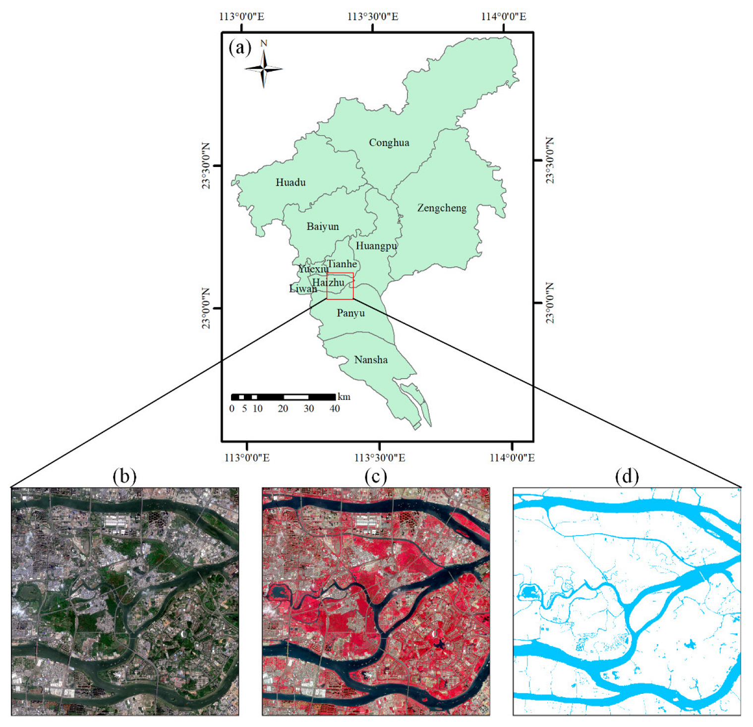
2.1. Study Area
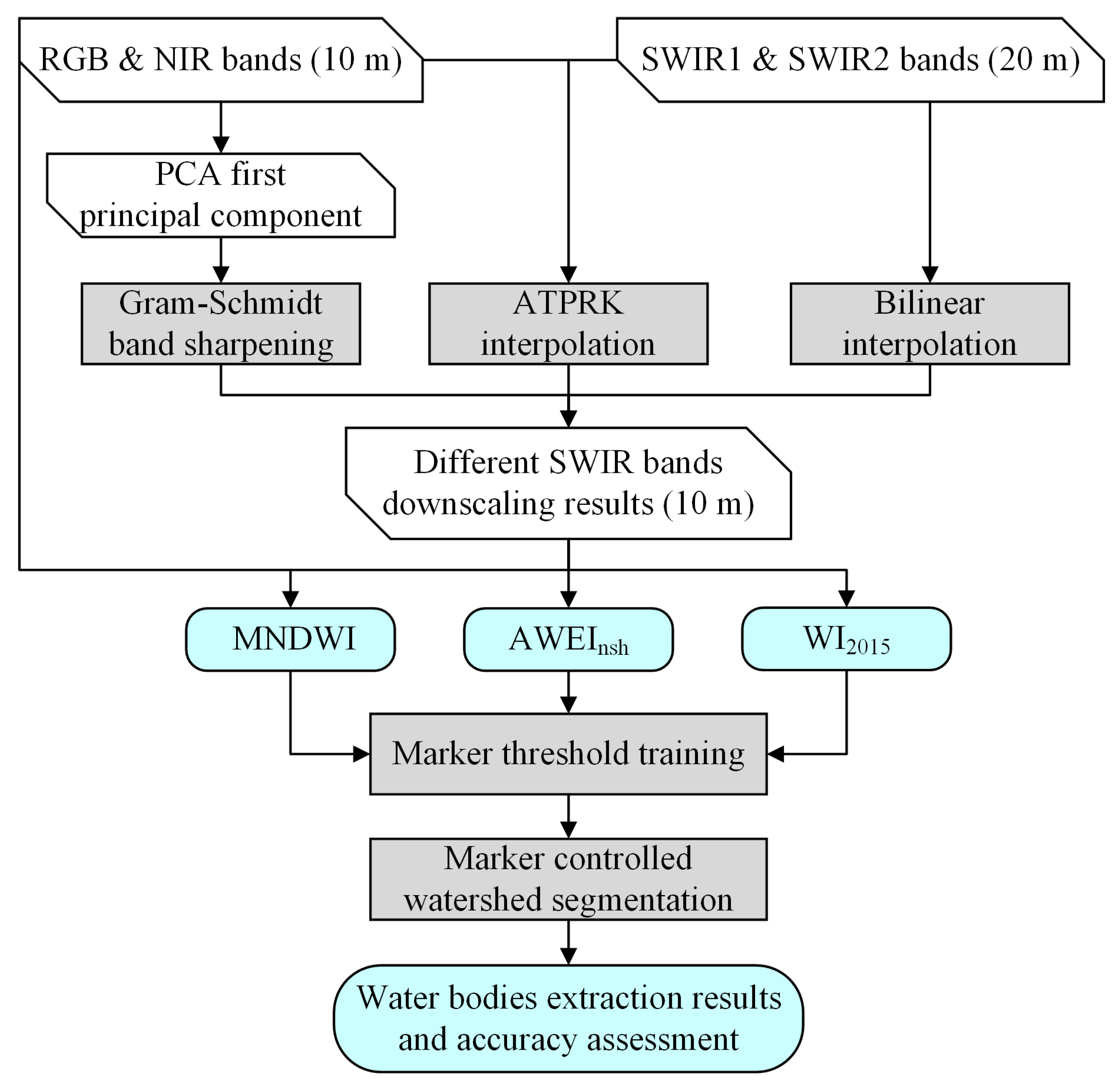
2.2. Methods
2.2.1. Water Indices
2.2.2. Gram–Schmidt Pan-Sharpening
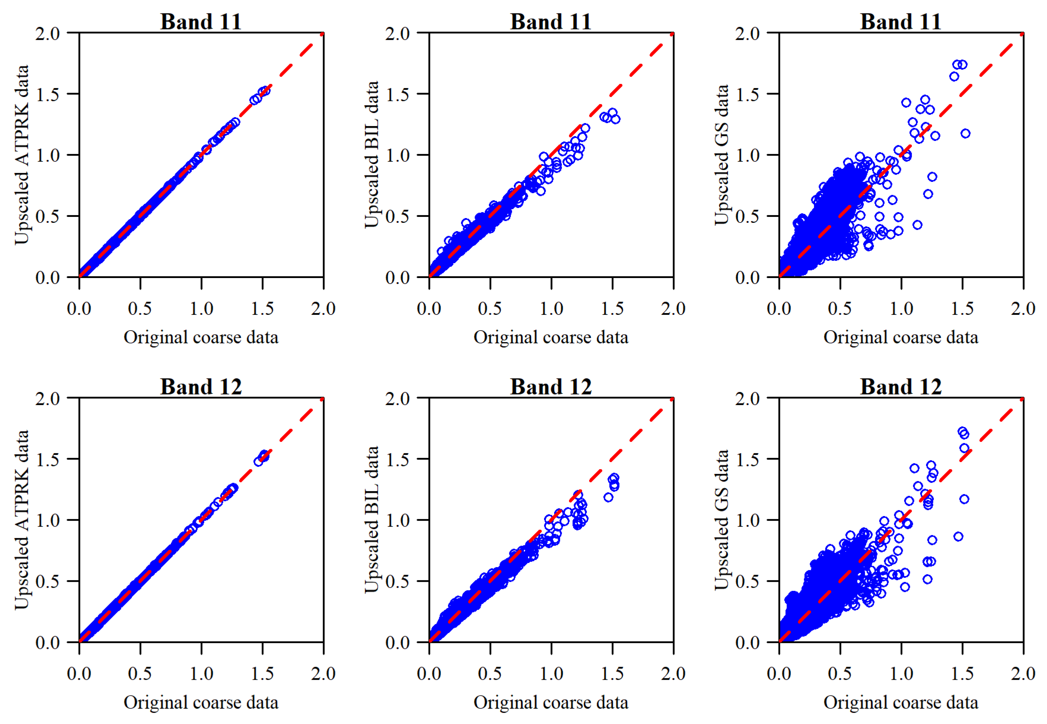
2.2.3. Area-to-Point Regression Kriging (ATPRK)
2.2.4. Marker-Controlled Watershed Segmentation
2.2.5. Accuracy Evaluation Indicators
3. Results
3.1. Band Downscaling Quality
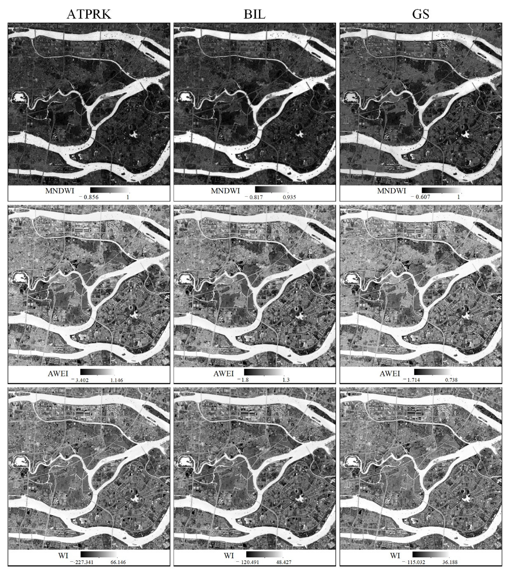
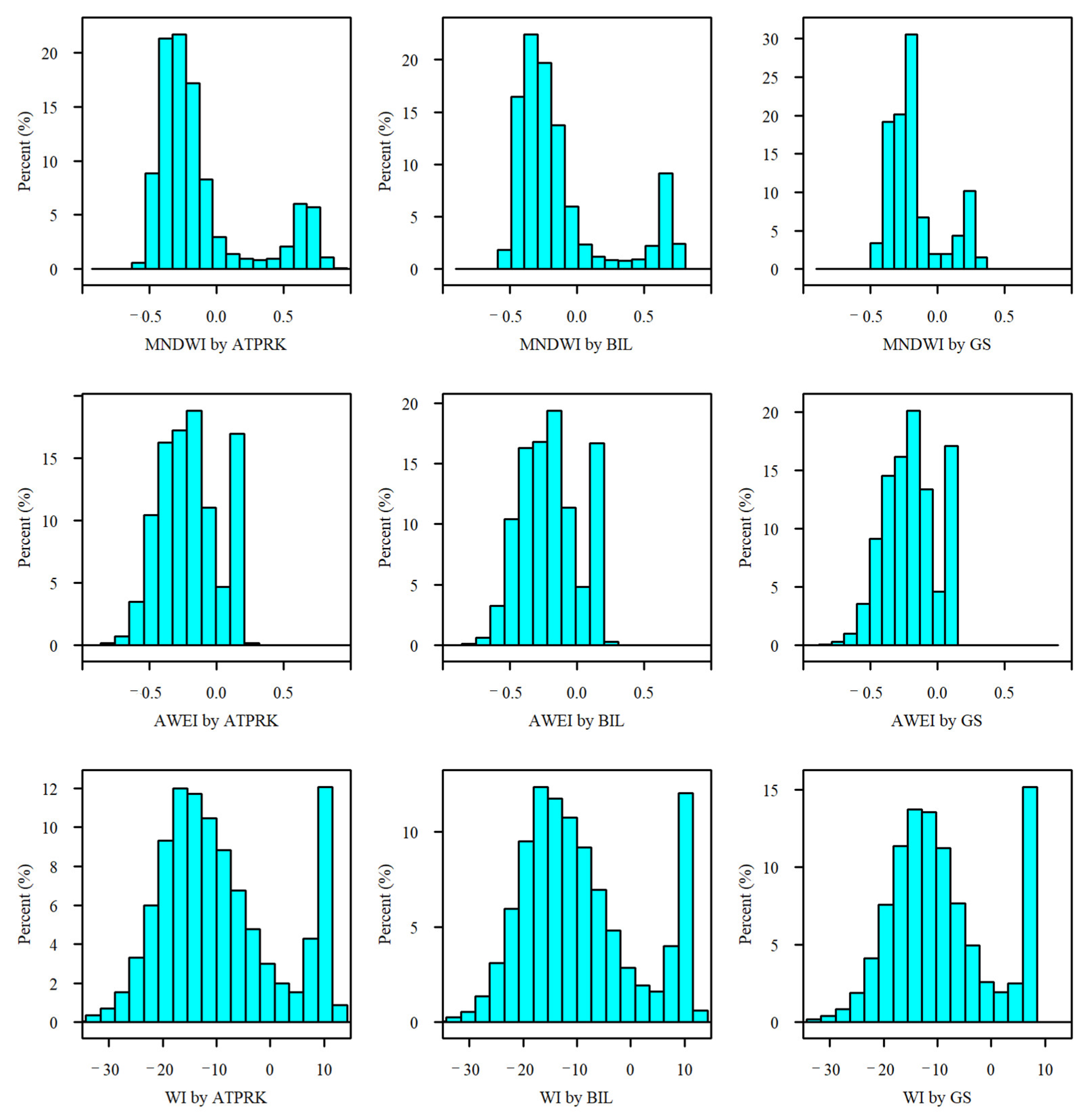
3.2. Water Indices Results
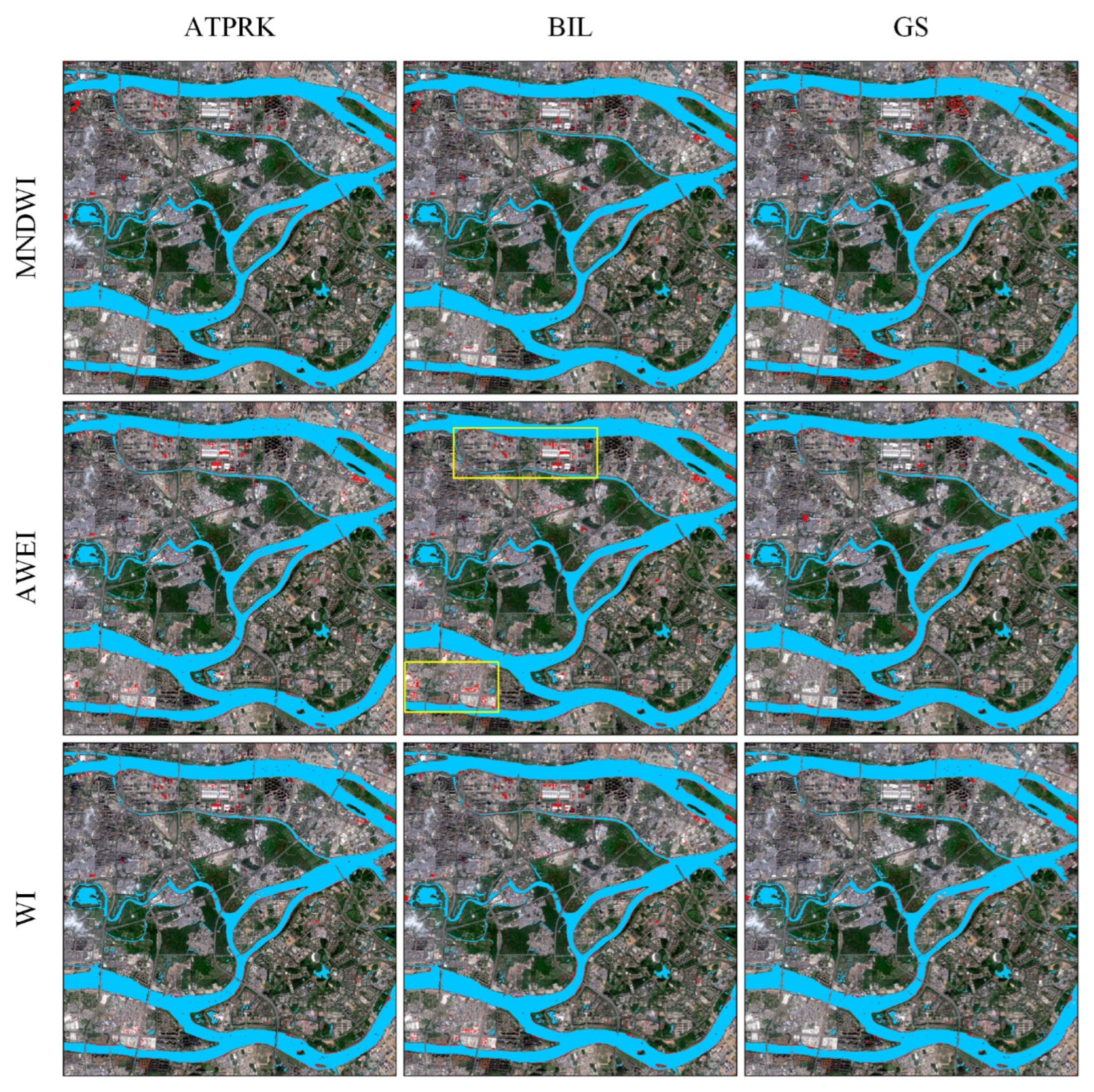
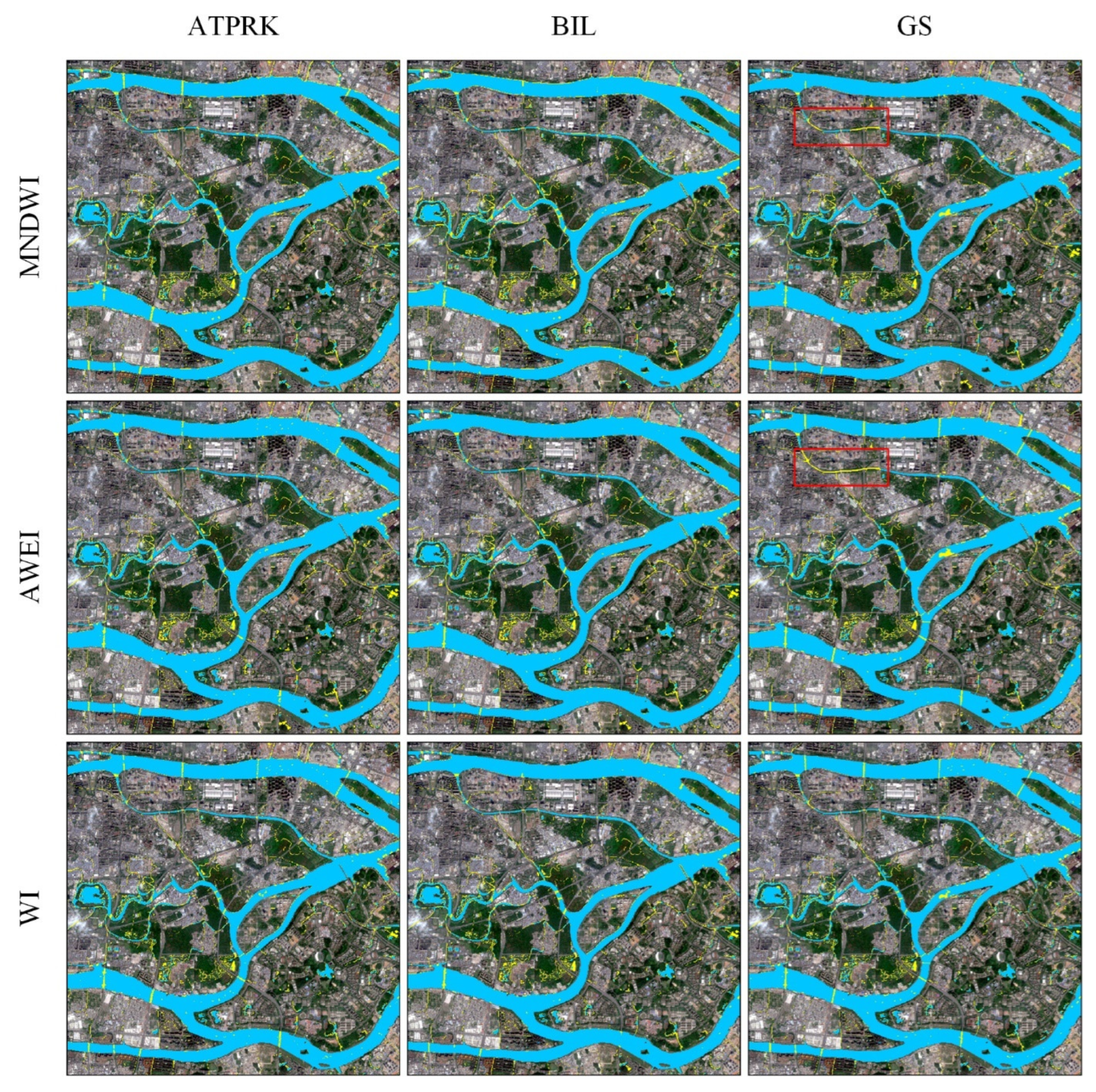
3.3. Analysis of Water Body Commissions and Omissions
3.4. Quantitative Evaluation of Water Body Extraction Accuracy
4. Conclusions
Author Contributions
Funding
Institutional Review Board Statement
Informed Consent Statement
Data Availability Statement
Acknowledgments
Conflicts of Interest
References
- Xie, H.; Luo, X.; Xu, X.; Pan, H.; Tong, X. Automated Subpixel Surface Water Mapping from Heterogeneous Urban Environments Using Landsat 8 OLI Imagery. Remote Sens. 2016, 8, 584. [Google Scholar] [CrossRef]
- Zhou, Y.A.; Luo, J.C.; Shen, Z.F.; Hu, X.D.; Yang, H.P. Multiscale Water Body Extraction in Urban Environments From Satellite Images. IEEE J. Sel. Top. Appl. Earth Obs. Remote Sens. 2014, 7, 4301–4312. [Google Scholar] [CrossRef]
- Huang, X.; Xie, C.; Fang, X.; Zhang, L.P. Combining Pixel- and Object-Based Machine Learning for Identification of Water-Body Types From Urban High-Resolution Remote-Sensing Imagery. IEEE J. Sel. Top. Appl. Earth Obs. Remote Sens. 2015, 8, 2097–2110. [Google Scholar] [CrossRef]
- Sun, X.; Tan, X.Y.; Chen, K.L.; Song, S.; Zhu, X.D.; Hou, D.L. Quantifying landscape-metrics impacts on urban green-spaces and water-bodies cooling effect: The study of Nanjing, China. Urban For. Urban Green. 2020, 55, 126838. [Google Scholar] [CrossRef]
- Du, N.; Ottens, H.; Sliuzas, R. Spatial impact of urban expansion on surface water bodies-A case study of Wuhan, China. Landsc. Urban Plann. 2010, 94, 175–185. [Google Scholar] [CrossRef]
- Pekel, J.-F.; Cottam, A.; Gorelick, N.; Belward, A.S. High-resolution mapping of global surface water and its long-term changes. Nature 2016, 540, 418–422. [Google Scholar] [CrossRef] [PubMed]
- Lehner, B.; Doll, P. Development and validation of a global database of lakes, reservoirs and wetlands. J. Hydrol. 2004, 296, 1–22. [Google Scholar] [CrossRef]
- Qi, B.; Zhuang, Y.; Chen, H.; Dong, S.; Li, L. Fusion feature multi-scale pooling for water body extraction from optical panchromatic images. Remote Sens. 2019, 11, 245. [Google Scholar] [CrossRef]
- Jiang, W.; Ni, Y.; Pang, Z.; Li, X.; Ju, H.; He, G.; Lv, J.; Yang, K.; Fu, J.; Qin, X. An effective water body extraction method with new water index for sentinel-2 imagery. Water 2021, 13, 1647. [Google Scholar] [CrossRef]
- Yue, H.; Li, Y.; Qian, J.; Liu, Y. A new accuracy evaluation method for water body extraction. Int. J. Remote Sens. 2020, 41, 7311–7342. [Google Scholar] [CrossRef]
- Chen, Y.; Tang, L.; Kan, Z.; Bilal, M.; Li, Q. A novel water body extraction neural network (WBE-NN) for optical high-resolution multispectral imagery. J. Hydrol. 2020, 588, 125092. [Google Scholar] [CrossRef]
- Li, L.; Yan, Z.; Shen, Q.; Cheng, G.; Gao, L.; Zhang, B. Water body extraction from very high spatial resolution remote sensing data based on fully convolutional networks. Remote Sens. 2019, 11, 1162. [Google Scholar] [CrossRef]
- Li, M.; Wu, P.; Wang, B.; Park, H.; Yang, H.; Wu, Y. A deep learning method of water body extraction from high resolution remote sensing images with multisensors. IEEE J. Sel. Top. Appl. Earth Obs. Remote Sens. 2021, 14, 3120–3132. [Google Scholar] [CrossRef]
- Yu, Y.; Yao, Y.; Guan, H.; Li, D.; Liu, Z.; Wang, L.; Yu, C.; Xiao, S.; Wang, W.; Chang, L. A self-attention capsule feature pyramid network for water body extraction from remote sensing imagery. Int. J. Remote Sens. 2021, 42, 1801–1822. [Google Scholar] [CrossRef]
- Shi, W.; Sui, H. An effective superpixel-based graph convolutional network for small waterbody extraction from remotely sensed imagery. Int. J. Appl. Earth Obs. Geoinf. 2022, 109, 102777. [Google Scholar] [CrossRef]
- McFeeters, S.K. The use of the normalized difference water index (NDWI) in the delineation of open water features. Int. J. Remote Sens. 1996, 17, 1425–1432. [Google Scholar] [CrossRef]
- Xu, H.Q. Modification of normalised difference water index (NDWI) to enhance open water features in remotely sensed imagery. Int. J. Remote Sens. 2006, 27, 3025–3033. [Google Scholar] [CrossRef]
- Feyisa, G.L.; Meilby, H.; Fensholt, R.; Proud, S.R. Automated Water Extraction Index: A new technique for surface water mapping using Landsat imagery. Remote Sens. Environ. 2013, 140, 23–35. [Google Scholar] [CrossRef]
- Fisher, A.; Flood, N.; Danaher, T. Comparing Landsat water index methods for automated water classification in eastern Australia. Remote Sens. Environ. 2016, 175, 167–182. [Google Scholar] [CrossRef]
- Sharma, R.C.; Tateishi, R.; Hara, K.; Luong Viet, N. Developing Superfine Water Index (SWI) for Global Water Cover Mapping Using MODIS Data. Remote Sens. 2015, 7, 13807–13841. [Google Scholar] [CrossRef] [Green Version]
- Wang, X.B.; Xie, S.P.; Zhang, X.L.; Chen, C.; Guo, H.; Du, J.K.; Duan, Z. A robust Multi-Band Water Index (MBWI) for automated extraction of surface water from Landsat 8 OLI imagery. Int. J. Appl. Earth Obs. Geoinf. 2018, 68, 73–91. [Google Scholar] [CrossRef]
- Liu, X.P.; Hu, G.H.; Chen, Y.M.; Li, X.; Xu, X.C.; Li, S.Y.; Pei, F.S.; Wang, S.J. High-resolution multi-temporal mapping of global urban land using Landsat images based on the Google Earth Engine Platform. Remote Sens. Environ. 2018, 209, 227–239. [Google Scholar] [CrossRef]
- Kaplan, G.; Avdan, U. Object-based water body extraction model using Sentinel-2 satellite imagery. Eur. J. Remote Sens. 2017, 50, 137–143. [Google Scholar] [CrossRef]
- Jiang, H.; Wang, M.; Hu, H.; Xu, J. Evaluating the Performance of Sentinel-1A and Sentinel-2 in Small Waterbody Mapping over Urban and Mountainous Regions. Water 2021, 13, 945. [Google Scholar] [CrossRef]
- Yang, X.; Zhao, S.; Qin, X.; Zhao, N.; Liang, L. Mapping of Urban Surface Water Bodies from Sentinel-2 MSI Imagery at 10 m Resolution via NDWI-Based Image Sharpening. Remote Sens. 2017, 9, 596. [Google Scholar] [CrossRef]
- Drusch, M.; Del Bello, U.; Carlier, S.; Colin, O.; Fernandez, V.; Gascon, F.; Hoersch, B.; Isola, C.; Laberinti, P.; Martimort, P.; et al. Sentinel-2: ESA’s Optical High-Resolution Mission for GMES Operational Services. Remote Sens. Environ. 2012, 120, 25–36. [Google Scholar] [CrossRef]
- Du, Y.; Zhang, Y.; Ling, F.; Wang, Q.; Li, W.; Li, X. Water Bodies’ Mapping from Sentinel-2 Imagery with Modified Normalized Difference Water Index at 10-m Spatial Resolution Produced by Sharpening the SWIR Band. Remote Sens. 2016, 8, 354. [Google Scholar] [CrossRef]
- Javan, F.D.; Samadzadegan, F.; Mehravar, S.; Toosi, A.; Khatami, R.; Stein, A. A review of image fusion techniques for pan-sharpening of high-resolution satellite imagery. ISPRS J. Photogramm. Remote Sens. 2021, 171, 101–117. [Google Scholar] [CrossRef]
- Chavez, P.S.; Kwarteng, A.Y. Extracting spectral contrast in Landsat thematic mapper image data using selective principal component analysis. Photogramm. Eng. Remote Sens. 1989, 55, 339–348. [Google Scholar]
- Carper, W.J.; Lillesand, T.M.; Kiefer, R.W. The use of intensity-hue-saturation transformations for merging spot panchromatic and multispectral image data. Photogramm. Eng. Remote Sens. 1990, 56, 459–467. [Google Scholar]
- Chavez, P.S.; Sides, S.C.; Anderson, J.A. Comparison of 3 different methods to merge multiresolution and multispectral data—Landsat TM and SPOT panchromatic. Photogramm. Eng. Remote Sens. 1991, 57, 295–303. [Google Scholar]
- Laben, C.A.; Brower, B.V. Process for Enhancing the Spatial Resolution of Multispectral Imagery Using PanSharpening. Available online: http://www.google.com/patents/US6011875 (accessed on 12 June 2017).
- Wang, Q.; Shi, W.; Atkinson, P.M.; Zhao, Y. Downscaling MODIS images with area-to-point regression kriging. Remote Sens. Environ. 2015, 166, 191–204. [Google Scholar] [CrossRef]
- Jiang, H.; Feng, M.; Zhu, Y.Q.; Lu, N.; Huang, J.X.; Xiao, T. An Automated Method for Extracting Rivers and Lakes from Landsat Imagery. Remote Sens. 2014, 6, 5067–5089. [Google Scholar] [CrossRef] [Green Version]


| Water Indices | Downscaling Methods | UA | PA | OA | Kappa |
|---|---|---|---|---|---|
| MNDWI | ATPRK | 95.02% | 86.79% | 96.45% | 0.885 |
| BIL | 94.12% | 84.84% | 95.92% | 0.867 | |
| GS | 93.55% | 87.56% | 96.31% | 0.882 | |
| AWEIsh | ATPRK | 92.32% | 87.81% | 96.11% | 0.876 |
| BIL | 91.51% | 87.40% | 95.87% | 0.868 | |
| GS | 93.80% | 88.70% | 96.57% | 0.891 | |
| WI2015 | ATPRK | 93.65% | 87.99% | 96.41% | 0.885 |
| BIL | 92.45% | 88.54% | 96.27% | 0.881 | |
| GS | 94.48% | 89.10% | 96.79% | 0.897 |
Publisher’s Note: MDPI stays neutral with regard to jurisdictional claims in published maps and institutional affiliations. |
© 2022 by the authors. Licensee MDPI, Basel, Switzerland. This article is an open access article distributed under the terms and conditions of the Creative Commons Attribution (CC BY) license (https://creativecommons.org/licenses/by/4.0/).
Share and Cite
Liu, H.; Hu, H.; Liu, X.; Jiang, H.; Liu, W.; Yin, X. A Comparison of Different Water Indices and Band Downscaling Methods for Water Bodies Mapping from Sentinel-2 Imagery at 10-M Resolution. Water 2022, 14, 2696. https://doi.org/10.3390/w14172696
Liu H, Hu H, Liu X, Jiang H, Liu W, Yin X. A Comparison of Different Water Indices and Band Downscaling Methods for Water Bodies Mapping from Sentinel-2 Imagery at 10-M Resolution. Water. 2022; 14(17):2696. https://doi.org/10.3390/w14172696
Chicago/Turabian StyleLiu, Haiyang, Hongda Hu, Xulong Liu, Hao Jiang, Wanxia Liu, and Xiaoling Yin. 2022. "A Comparison of Different Water Indices and Band Downscaling Methods for Water Bodies Mapping from Sentinel-2 Imagery at 10-M Resolution" Water 14, no. 17: 2696. https://doi.org/10.3390/w14172696