Rainstorms Inducing Shifts of River Hydrochemistry during a Winter Season in the Central Appalachian Region

Abstract

Rainstorms rapidly change catchment conditions which can alter river flow and water constituents due to the transport and fate of suspended and dissolved solids and the river water chemistry. To understand river water chemistry changes, this investigation relies on field data collected during a winter season. The Kanawha River in West Virginia was monitored using grab water samples and continuous readings from two water quality stations (Q1 and Q2) separated by 23.5 km. Water samples allowed the identification of water chemistry, whereas the two stations retrieved hourly measurements of temperature, turbidity, NO₃⁻, Cl⁻ and pH to capture transient rainstorm responses. It was found through the Piper diagram that water type was mainly calcium-chloride, whereas the Gibbs diagram identified that the dominant geochemical process was rock weathering. On the other hand, during transient rainstorms responses, we found that concentrations of HCO₃⁻, NO₃⁻ and Cl⁻ changed from bicarbonate type to no dominant type. Furthermore, hysteretic effects of rainstorms were influenced by the soil moisture of the catchment area. Additionally, HCO₃⁻ and NO₃⁻ had different hysteretic loop directions between Q1 and Q2. This approach proved that river water chemistry adjustments caused by rainstorms were successfully identified by relying on grab water samples and continuous measurements.

1. Introduction

An accurate spatiotemporal hydrochemistry description of a river within a catchment area represents a challenge. The soil composition, vegetation, topography, climate and anthropogenic factors of the catchment strongly intervene in the definition of the river water chemistry. Even more, the relationship between catchment characteristics and the hydrologic cycle becomes a continuous adjustment of water budget and water chemistry as the drainage area along streams and rivers increases and heterogeneous spatial and temporal precipitation occurs. Thus, water in a catchment causes a convoluted pattern for the transport and fate of water constituents that may reshape biogeochemical processes [1] that subsequently change water chemistry. The impact of each rainstorm, based on the frequency, intensity and duration, causes particular changes of the water budget during an extent of time and applied to a particular catchment section. Within the catchment, water takes different paths such as evapotranspiration, surface runoff, infiltration, percolation, and the resulting surface water could be combined with current subsurface and underground water. As a consequence, water advancing downstream and converging in streams and rivers also adjusts the biotic and abiotic components [2,3]. These intricate field catchment conditions regulate the spatial and temporal variability of draining water that ultimately define the regime of river hydrochemistry changes.

Water chemistry in rivers is consistently associated with the type of sediments observed in the catchment. It is related with the impact of anthropogenic factors such as agriculture, surface mining and urban areas [4]. In addition, the precipitation regime collects and transports sediments downstream from upper regions which also facilitates simultaneous mixing and dissolution. This is happening due to low ionic concentrations that may prevail in water from precipitation in the Appalachian Region [5,6]. When water and sediments are mixed in streams and rivers, dams and locks together with hydropower operations can likewise influence the sediment dynamic patterns between storage and flushing. Furthermore, the transport and fate of sediments in rivers continuously change composition related with total suspended solids (TSS) and total dissolved solids (TDS). TSS includes large particles floating under turbulent conditions, whereas TDS are ionic compounds immersed in water. Even though TDS and TSS are related and exchanges between them exist, the ratio of the two terms cannot be accurately represented [7], making it more challenging under the impact of rainstorms.

TSS estimations are feasible under a robust approach associated with the flow [8]. For this study, we applied the TSS–flow relationship by means of the power-law equation [9]. Furthermore, increasing the reliability of TSS estimations required an in situ calibration with grab water samples [10]. On the other hand, estimations of TDS were achieved through water chemistry of in situ grab water samples. In particular, ions characterizing TDS were used to identify the type of water chemistry by means of the Piper diagram [11] and also the interpretation of the source’s water constituents by means of the Gibbs diagram [12].

Although the type of water chemistry may characterize a river, rainstorms cause temporal changes. To understand how transient rainstorm responses affect the flow and concentration of ions, this study utilized the concentration (c) of three anions (HCO₃⁻, NO₃⁻ and Cl⁻) and their relationship with flow (q). Such an approach allowed us to obtain further information by applying the hysteresis concept to the c–q relationship [13]. Hysteresis explains the capacity of a rainstorm on a river for the transport, dispersion and deposition of ions based on the catchment field conditions [14,15]. Nevertheless, hysteresis may depend on initial conditions, making it necessary to know catchment wetness conditions at the onset of the rainstorm event [16]. Estimations of the catchment wetness conditions then relied on the estimated soil moisture conditions [17,18] as a consequence of the anticipated precipitation regime [19]. In this way, initial conditions of the catchment area for each rainstorm can be established.

We focused on the Kanawha River in West Virginia, which is one of the tributaries of the Ohio River in the Central Appalachian Region. The drainage area of the Kanawha River includes a dense chemical industry near urban areas settled for more than a century as well as mining activities for coal and shale gas that altogether caused significant water pollution [4,20,21,22,23]. These anthropogenic activities discharge wastewater to streams together with scattered agriculture runoffs from riverine zones. Therefore, this drainage area has been subjected to local discharges such as the national pollutant discharge elimination system (NPDES). The Kanawha River encompasses approximately 31,724 km² with many types of wastes, hypoxic conditions and endangering aquatic ecosystems [23]. The effects of rainstorms in this study area were investigated taking into account water chemistry changes that propagate downstream and may impair aquatic life conditions and the adequacy of water for different uses.

This research combined experimental and modeling datasets of the water chemistry, hydrology and hydrodynamics of a river in order to assess changes of hydrochemistry due to rainstorms. Furthermore, two locations along the Kanawha River served to keep track of changes through the transient conditions of rainstorms. Accordingly, this research addressed the following objectives: (1) identification of the river water chemistry, (2) estimation of hydrochemistry changes due to rainstorms, and (3) analysis of transient rainstorm responses of anions.

2. Materials and Methods

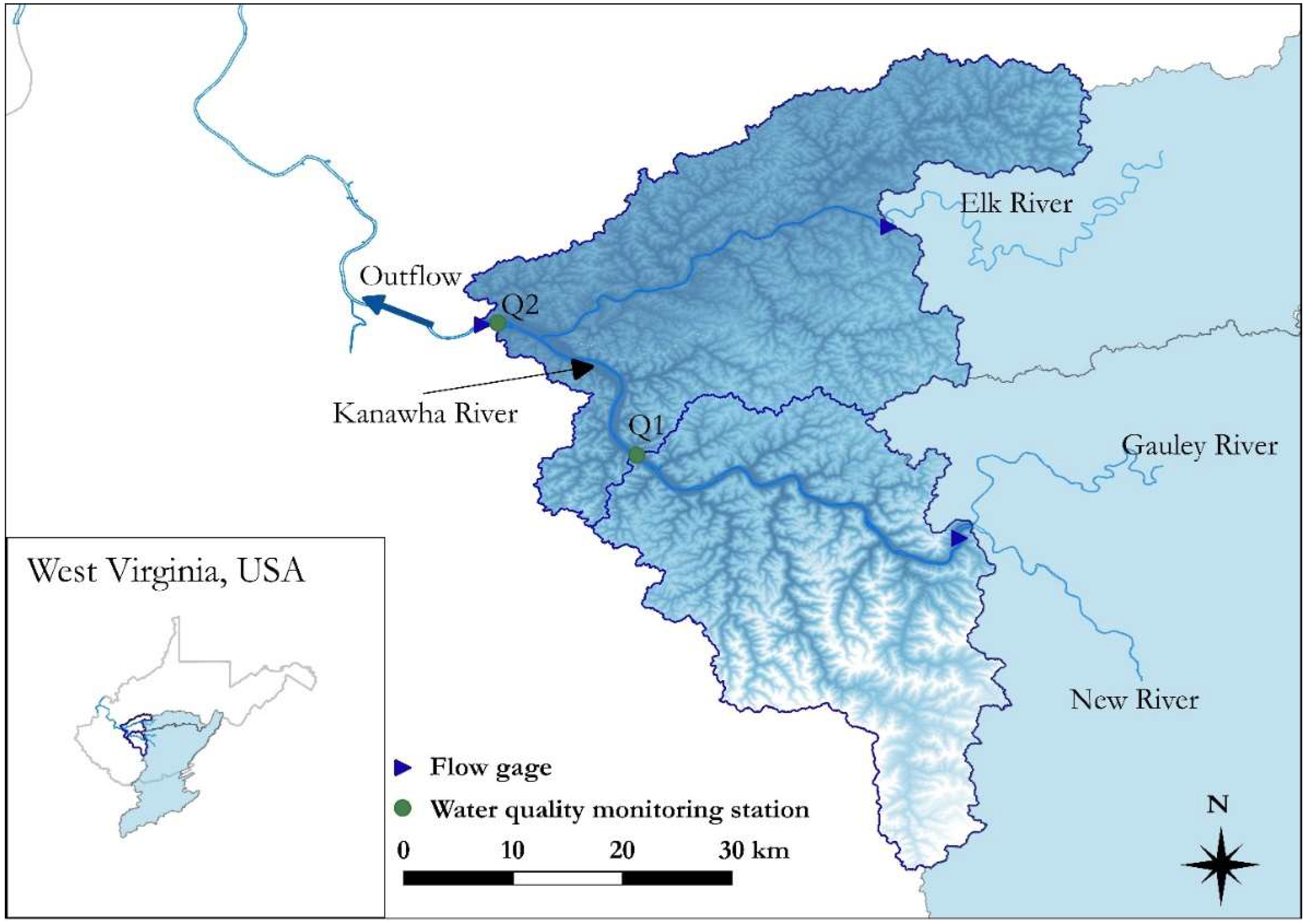
2.1. Description of the Study Area

The Kanawha River (Figure 1) is located in the Central Appalachian Region. However, the New River with a catchment area of 18,026 km² becomes the Kanawha River in latitude 38.160° N and longitude 81.197° W. The Kanawha River has a length of 156 km with the Elk River as a tributary of the Kanawha River, which flows into the Ohio River. Elevation of the Kanawha River starts and ends at 228.5 and 176 m above sea level, respectively. USGS flow measurements in the Kanawha River at the site 03198000 [24] had a mean annual flow of 442 m³/s oscillating between the lowest (31 m³/s) and highest (4530.7 m³/s) mean daily flow.

The catchment is composed of forest (75.5%), agriculture (13.5%), developed (6.3%), herbaceous (1.9%), shrubland (1.4%), surface water and wetland (0.8%) and barren (0.6%), according to the National Land Cover Database [25] of the USA. Soils of the study area are moderately deep containing sandstone, shale, coal and siltstone allowing moderate drainage. Regions with shale soils are commonly loamy and silty, whereas limestone soils are commonly silty and clayey [26]. Mountain soils are more related to be sandstone and shale rocks, according to [27].

Within this catchment, the mean annual precipitation is 1107 mm, which is computed from 1948–2020 using the NASA GLDAS database [17,18]. Contributions of precipitation impacting flow are mostly observed at the end of winter and beginning of spring. In addition, high flows are staggered through the year with more frequency during summer and fall due to seasonal rain. From winter to summer, the mean air temperature ranges from −3 to 30 °C.

The Q1 and Q2 locations (Figure 1) comprised a drainage area of 22,769.8 and 27,060.2 km², respectively. Q1 was located at 38.2243° N, 81.5356° W and Q2 was located at 38.3625° N, 81.6642° W. The distance between Q1 and Q2 locations following the Kanawha River path was 23.5 km, which included the Elk River as the main tributary. In addition, the mean river slope and width for section Q1–Q2 were 0.00004 and 175 m, respectively.

2.2. Chemical Analysis of Grab Water Samples

A set of 45 grab water samples was retrieved and used for analyzing major ions during the period February 2016–September 2018, with sampling dates and GPS coordinates provided in Supplementary Information Table S1. This set of water samples was collected in acid-washed 1 L HDPE bottles that were previously rinsed with river water before collection. Samples were collected >5 m from the shore in the Q2 location and taken to the Soil Science Laboratory at the West Virginia State University to be kept under refrigeration (4 °C). Major ions (Cl⁻, NO₂⁻, NO₃⁻, F⁻, K⁺, SO₄²⁻, PO₄⁻, Na⁺, K⁺, NH₄⁺, Mg²⁺ and Ca²⁺) were estimated using the ion chromatography system (Dionex ICS-1100, Thermo Fisher Scientific, Waltham, MA, USA), whereas soluble metals (Fe, Mn and Al) were measured with an inductively coupled plasma optical emission spectrometer using ICP-OES (Optima 8000 ICP-OES, Perkin Elmer, Waltham, MA, USA).

Estimation of HCO₃⁻

Dissolved inorganic carbon (DIC) mainly describes CO₂ + H₂CO₃ + HCO₃⁻ + CO₃²⁻. However, for 6.4 > pH > 10.3, contributions of CO₂ and H₂CO₃ are reduced significantly, approximating DIC to be HCO₃⁻ + CO₃²⁻ [28]. In our study area, a mean pH of 6.8 [4] (also verified with pH measurements in Section 3.3) implied that HCO₃⁻ represented >90% of the carbonates according to the Bjerrum plot [28]. In order to estimate HCO₃⁻, we used the CO2Sys [29], which relied on pH and pCO₂. pH was measured in the river and pCO₂ was estimated based on [30]. Then, HCO₃⁻ of the 45 water samples was estimated with great simplification of all phenomena related to CO₂ fluxes [31,32,33].

2.3. High-Frequency Data of a Hydrologic Model and Water Quality Monitoring Stations

Field surveys were conducted in the period 21 December 2017–22 March 2018. Two monitoring stations (Q1 and Q2 indicated in Figure 1), using Eureka Manta 2 multi-probe sondes, were deployed along the river. Each monitoring station hourly measured pH (±0.2), temperature (±0.1 °C), NO₃⁻ (±10%), Cl⁻ (±10%), and turbidity (±3%, NTU). The stations served to estimate TSS through flow. HCO₃⁻ was calculated through pH, water temperature, atmospheric pressure and mean pCO₂ [30] following the CO2Sys [29]. Hourly estimations of flow in the Kanawha River in the two locations (Q1 and Q2) were deduced from a developed and calibrated HSPF hydrologic model [23]. In addition, the Q2 differed with respect to Q1 due to the additional 4290.4 km² of drainage area to the Kanawha River, representing an increase in mean flow up to 17% when compared to Q1 [23].

2.4. Soil Moisture

Each rainstorm impact depended on the catchment draining capacity, which is related to slope, land use and soil moisture. Nonetheless, slope and land use within a season were steady, whereas soil moisture was not. This study addressed the effect of soil moisture as the driving factor to drain water to the river before each rainstorm; estimations of soil moisture at a daily time step were collected from NASA GLDAS [34] for the period 21 December 2017–22 March 2018.

2.5. Hysteresis Index (HI)

The river flow fluctuations followed by corresponding concentrations of dissolved solids, denoted as c–q, are distinctive for each catchment [1,8,35]. The c–q relationship identifies different responses which are associated with the type of rainstorm and catchment characteristics such as land use, soil and anthropogenic activities [1,36]. The c–q relationship for specific rainstorms flushing into the river as a cyclical phenomenon is adequately represented by hysteresis. Patterns of hysteresis cover a period from the minimum flow (equal to 0) to the rising limb as time advances until the maximum flow (equal to 1); then, it follows the falling limb until it reaches the minimum flow (equal to 0). The hysteresis loop is dimensionless and is deduced from normalized concentration ($c_i$) and flow ($q_i$), as indicated in Equation (2).

$$\overline{q_i}=\frac{\left(q_i-q_{max}\right)}{\left(q_{max}-q_{min}\right)}$$

(1)

$$\overline{c_i}=\frac{\left(c_i-c_{max}\right)}{\left(c_{max}-c_{min}\right)}$$

(2)

where $q_i$ and $c_i$ are the instantaneous flow discharge and concentration in time step i. The $q_{min}$, $q_{max}$, $c_{min}$ and $c_{max}$ are minimums and maximums of the flow discharge (q) and concentration (c) during a specific rainstorm event. In order to know the loop shape and direction, we used the hysteresis index ($HI$) which ranges from −1 to 1 (Equation (3)). Since HI is subjected to local changes, it was computed at increments of 0.05, which is a recommended interval by [37]; therefore, each rainstorm deduced a $H{I}_{mean }$ and $H{I}_{std dev }$ from 0.1 to 0.9 of the normalized discharge. Values of HI < 0 implied an anticlockwise loop direction, HI near to 0 implied complex hysteresis and HI > 0 implied a clockwise loop direction.

$$HI={\overline{c}}_{i RL}-{\overline{c}}_{i FL}$$

(3)

where ${\overline{c}}_{i RL}$ and ${\overline{c}}_{i FL}$ correspond to the normalized concentration on the rising limb and falling limb, respectively.

2.6. Total Suspended Solids (TSS)

TSS were retained after filtering out with pore size equal to 2 μm. TSS may contain sand, silt, clay, minerals and biological matter that are found in high concentrations under water turbulence conditions. In contrast, TDS were passing through the same filter, which were analyzed through major ions. The temporal variation of the ratio of TSS with respect to TDS during rainstorms may not be well defined [7]; therefore, an alternative is TSS as a function of the river hydrodynamics.

To resolve TSS estimations, we considered that rainstorms have a particular and recurrent response in TSS as consequence of the changes of river flow, according to the characteristics of the catchment [38]. To accomplish that, the TSS of grab water samples were measured in the lab following the guidelines stated in Standard Methods [39]. Flow was determined using a hydrologic model (HSPF) for the Kanawha River [23]. This study estimated TSS with a set of 62 water samples with three replicates. The relationship between TSS and flow was established through the power-law equation (Equation (4)).

$$TSS \left(q\right)=a{q}^b$$

(4)

where coefficients a and b correspond to the adjustment of TSS to the flow q.

3. Results and Discussion

3.1. Hydrochemistry of Water Samples

Summary of the water chemistry through mean values of cations and anions of the Kanawha River at location Q2 are introduced in

Table 1. Summary of the water chemistry analysis of 45 grab water samples.

	K+	Mg2+	Ca2+	Na+	Cl−	SO42−	NO3−	HCO3−
Mean	2.18 (±1.69)	7.22 (±2.35)	20.14 (±2.72)	6.40 (±1.45)	6.85 (±2.07)	34.33 (±9.00)	2.17 (±0.71)	12.34 (±1.49)
Min	1.26	1.30	14.65	4.06	3.75	22.57	1.15	9.97
Max	6.89	10.19	23.74	9.75	10.48	50.30	3.11	15.66

Note: All units in mg/L.

, with a predominance of cations in the order Ca²⁺ > Mg²⁺ > Na⁺ > K⁺ with 55%, 20%, 18% and 7%, respectively. The predominance of anions was in the order SO₄²⁻ > HCO₃⁻ > Cl⁻ > NO₃⁻ with 62%, 22%, 12% and 4%, respectively. To verify the reliability of ions balance in these water chemistry analyses, we conducted a comparison of total cations and anions (in meq), which had a correlation of R² equal to 0.95.

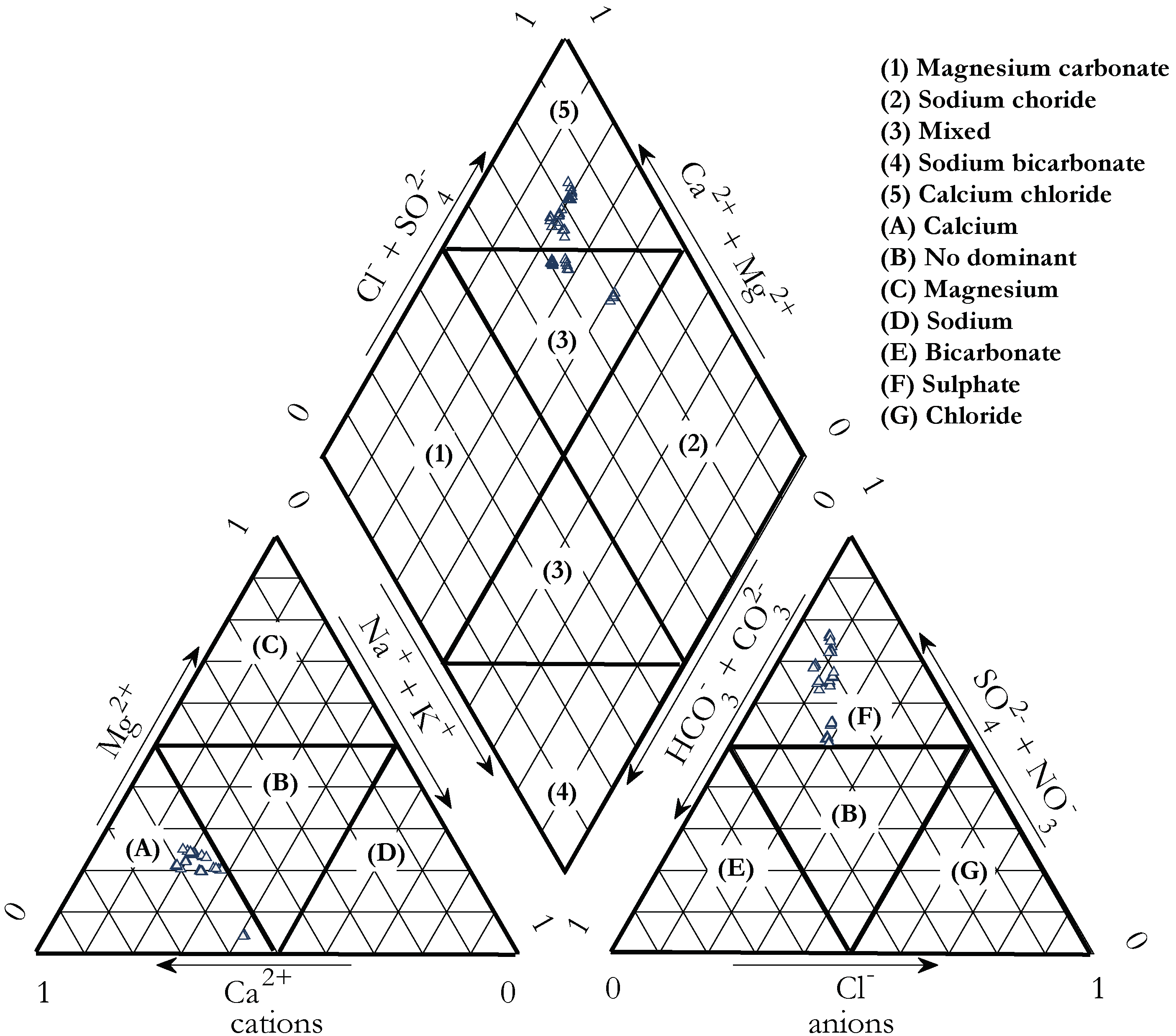
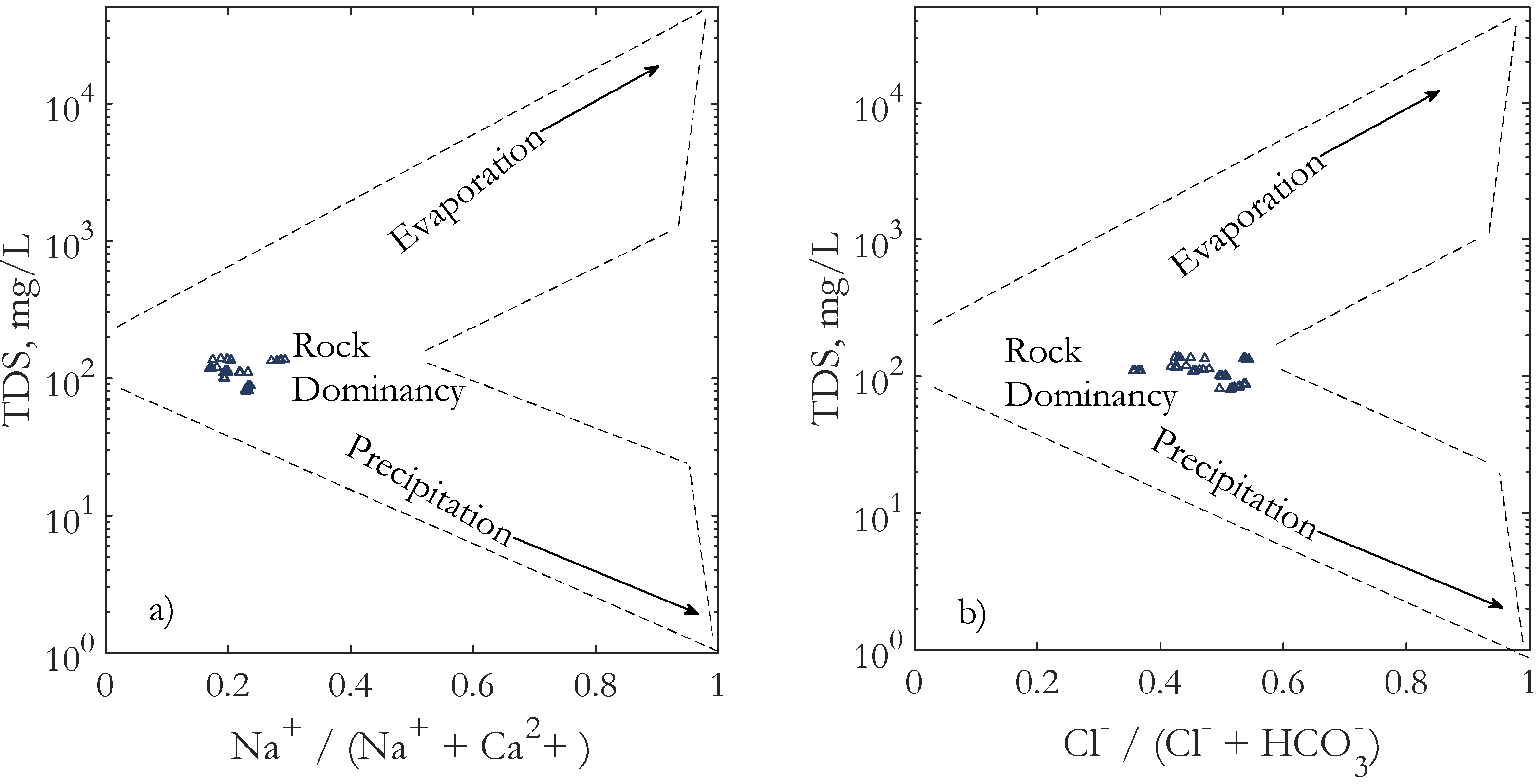
3.2. Hydrochemical Facies and Origin of Dissolved Solids

All major ions indicated in Table 1 were converted to meq (%) and plotted in the Piper diagram. Cations and anions diagrams were projected into a combined anions–cations diamond plot (Figure 2). Hydrochemical facies aided in the classification of the water chemistry type. A cations diagram had a prevalent dominance of Ca²⁺ combined with contributions between 15% and 30% of Na⁺ + K⁺ and between 35% and 50% of Mg²⁺. The anions diagram remarkably indicated that water samples fall on the upper corner, implying a SO₄²⁻ dominated lithology; however, those water samples also defined ranges within 5% and 20% for Cl⁻ and within 15% and 30% for HCO₃⁻. Based on the central diamond, water samples were identified as calcium-chloride. In addition, those water samples had alkaline earth elements (Ca²⁺ and Mg²⁺) exceeding alkalis (Na⁺ and K⁺). Furthermore, the strong acids (Cl⁻ and SO₄²⁻) were dominant over weak acids (HCO₃⁻).

A Gibbs diagram (Figure 3) identified that Na⁺/(Na⁺ + Ca²⁺) was between 0.15 and 0.3 and Cl⁻/(Cl⁻ + HCO₃⁻) was between 0.35 and 0.55 when dealing with TDS between 50 mg/L and 120 mg/L. In addition, the Gibbs diagram indicated that rock weathering mainly contributed to the composition of TDS with respect to other mechanisms such as biota, discharges of pollutants to the river and effects of precipitation.

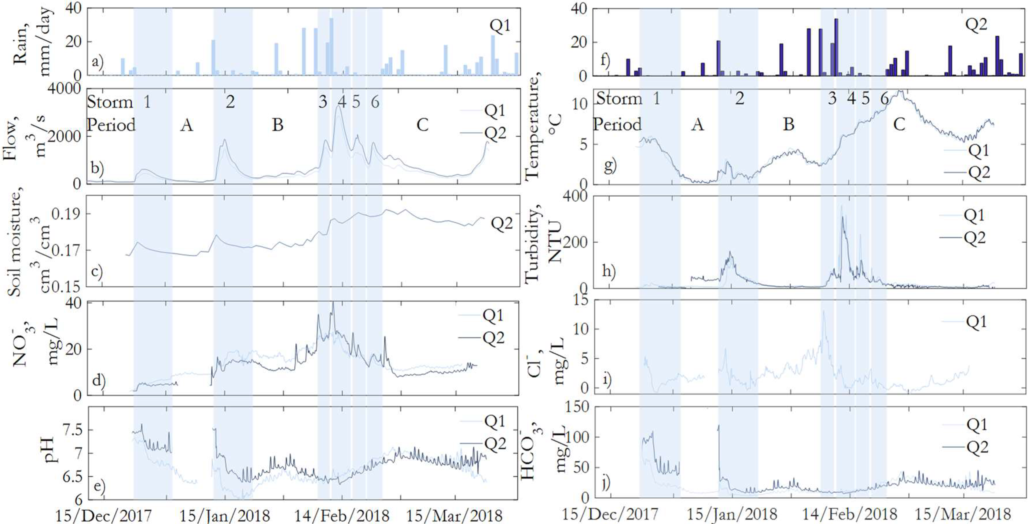
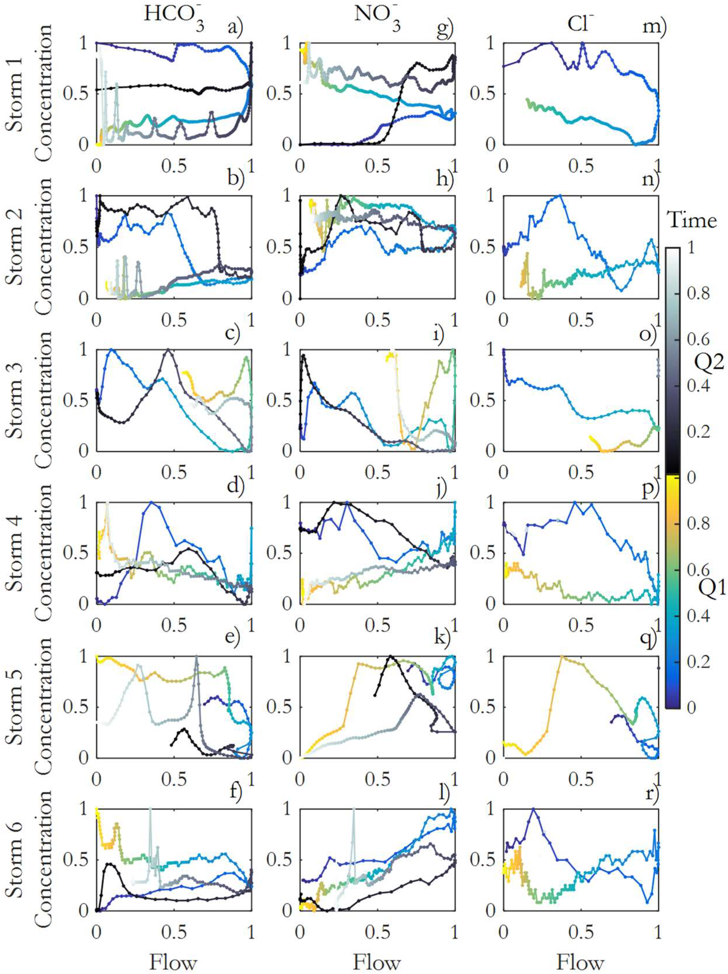
3.3. Hydrochemistry under High-Frequency Data

Catchment characteristics (Figure 1) and climate data were used to estimate flow (Figure 4b) following a developed HSPF hydrologic model. The HSPF hydrologic model was calibrated and validated to predict flow in Q1 and Q2, having a performance of NSE and PBIAS equal to 0.96 and 1.97%, respectively; further information of this HSPF model is available in [23]. Precipitation (Figure 4a,b) was retrieved from the near-real-time precipitation TRMM model [40]. Measurements of temperature, turbidity, NO₃⁻, Cl⁻ and pH (Figure 4d,e,g,i) were collected from the multi-probe sondes whereas soil moisture (Figure 4c) from the NASA GLDAS database and HCO₃⁻ (Figure 4i) was estimated using CO2Sys. During the period of observation, six rainstorms were identified using time series datasets which were intercalated with periods A, B and C (Figure 4b). The bounds at the start and end of each rainstorm were defined based on the minimum flow q. Each rainstorm was characterized through mean starting, maximum and ending flow, and duration of the rainstorm event (

Table 2. Characteristics of six rainstorms at Q1 and Q2 locations along the Kanawha River.

Location	Storm	Starting Flow (m3/s)	Maximum Flow (m3/s)	Ending Flow (m3/s)	Time to Reach Maximum Flow (h)	Event Duration (h)
Q1	1	132	449	100	59	339
	2	128	1395	213	62	240
	3	515	1542	1090	46	84
	4	1065	2825	1089	41	118
	5	1129	1335	659	30	93
	6	643	1518	748	32	108
Q2	1	157	617	107	61	339
	2	146	1729	268	83	270
	3	662	1849	1363	48	86
	4	1310	3231	1362	40	118
	5	1444	2083	849	28	94
	6	816	1764	1036	31	108

).

Mean concentrations of HCO₃⁻ (

Table 3. Mean concentrations of anions during rainstorms and periods in between indicated in Figure 4.

	HCO3−, mg/L		NO3−, mg/L		Cl−, mg/L
	Q1	Q2	Q1	Q2	Q1
Storm 1	23.4 (±15.4)	61.6 (±7.1)	6.9 (±1.8)	4.5 (±0.6)	6.5 (±1.2)
Period A	8.9 (±3.1)	-	9.4 (±0.2)	4.4 (±0.1)	7.2 (±0.6)
Storm 2	6.4 (±3.7)	19.2 (±16.5)	16.3 (±2.7)	13.1 (±2.5)	6.6 (±1.4)
Period B	5.6 (±1.6)	11.7 (±3.3)	17.9 (±2.2)	13.6 (±3.1)	9 (±2.1)
Storm 3	9.4 (±0.8)	9.4 (±0.7)	25.3 (±0.9)	27.5 (±3.7)	9.9 (±2.9)
Storm 4	12.2 (±1.6)	9.6 (±1.4)	21.5 (±3.4)	26.4 (±5.5)	6 (±1.1)
Storm 5	15.5 (±1.6)	14.1 (±1.6)	16.3 (±1.4)	18.4 (±3.5)	6.5 (±0.7)
Storm 6	25.2 (±3.7)	20.5 (±2.4)	14.1 (±1.8)	15.8 (±2.8)	5.3 (±0.4)
Period C	18.8 (±6.4)	18.3 (±4.2)	11.9 (±0.7)	10.5 (±1.8)	5.8 (±0.4)

) of rainstorms were found to be higher with respect to the mean concentration observed in intercalated periods in either Q1 or Q2 locations. In addition, the mean concentrations of HCO₃⁻ in rainstorms 1–3 were equal or higher in Q2 than Q1. In contrast, the mean concentrations in rainstorms 4–6 were lower in Q2 than Q1. However, NO₃⁻ showed a continuous increase having the maximum in storm 4 and Cl⁻ and followed a similar pattern having the maximum in storm 3; then, both ions concentrations were falling down by the end of the period of observation.

Comparison between Water Samples and Continuous Monitoring

It was found that the mean concentration during continuous monitoring of HCO₃⁻ and NO₃⁻ changed significantly between the monitoring stations Q1 and Q2 (

Table 4. Mean concentrations of HCO₃⁻ and NO₃⁻ from water samples and continuous monitoring.

	HCO3−, mg/L		NO3−, mg/L		Mean Soil Moisture, cm3/cm3	Mean Flow, m3/s
	Q1	Q2	Q1	Q2
Water Samples *	-	12.36 (±1.48)	-	2.15 (±0.71)	0.180 (±0.01)	239.3 (±74)
Monitoring stations	13.91 (±9.52)	20.63 (±19.99)	14.05 (±5.47)	12.45 (±6.68)	0.185 (±0.007)	696.7 (±608)

Note: * Mean soil moisture and flow were retrieved from [22] and [32] based on the sampling days of grab water samples.

) due to the potential effects of local discharges. On the other hand, water samples near Q2 had lower concentrations of HCO₃⁻ and NO₃⁻ with respect to continuous monitoring. The discrepancy of water samples and continuous monitoring had happened, since water samples occurred with different catchment and river conditions such as the soil moisture and flow (Table 4); nonetheless, other factors such as heterogeneous spatial and temporal precipitation within the catchment (Supplementary information, Figure S1 and Table S1) had intervened, too.

3.4. Hysteresis of Anions

Rainstorms were normalized and analyzed through the c–q relationship. Comparison between Q1 and Q2 was possible for all rainstorms except for c–q of Cl⁻. In addition, it was observed that at the end of various rainstorms in Q2 (e.g., Figure 5a), one or more peaks were present, which were attributed to local discharges such as NPDES.

Dynamics of mobilization of HCO₃⁻, NO₃⁻ and Cl⁻ were driven differently at each rainstorm (Figure 5). For instance, HCO₃⁻ in any rainstorm followed the same loop direction in Q1 and Q2. Rainstorms 1, 2 and 4 (Figure 5a–f) followed a clockwise hysteretic loop direction (HI > 0, Table 4), and rainstorms 3, 5 and 6 a counterclockwise hysteretic loop direction (HI < 0). Nonetheless, values of HI were progressively moving from HI > 0 to HI < 0 as rainstorms successively occurred in Q1 and Q2. Values in the range −0.07 ≤ HI ≤ −0.16 indicated a marginal hysteretic effect and could be classified as complex [14]. Additionally, HI magnitude consistently decreased (

Table 5. Hysteresis index (HI) of HCO₃⁻, NO₃⁻ and Cl⁻ for the rainstorms in the locations Q1 and Q2 along the Kanawha River.

	$\mathbf{H}\mathbf{I}{ }_{\left(\pm \mathit{s}\mathit{t}\mathit{d} \mathit{d}\mathit{e}\mathit{v}\right) }$
	HCO3−		NO3−		Cl−
Storm	Q1	Q2	Q1	Q2	Q1
1	0.71 (±0.06)	0.38 (±0.18)	−0.35 (±0.21)	−0.30 (±0.25)	0.61 (±0.06)
2	0.52 (±0.37)	0.14 (±0.06)	−0.44 (±0.11)	−0.12 (±0.16)	0.33 (±0.35)
3	−0.44 (±0.13)	−0.07 (±0.17)	−0.29 (±0.37)	−0.26 (±0.29)	0.32 (±0.04)
4	0.16 (±0.33)	0.03 (±0.16)	0.35 (±0.26)	0.47 (±0.16)	0.60 (±0.21)
5	−0.16 (±0.20)	−0.16 (±0.29)	−0.04 (±0.06)	0.24 (±0.31)	−0.21 (±0.13)
6	−0.30 (±0.24)	−0.21 (±0.21)	0.09 (±0.14)	−0.34 (±0.27)	0.15 (±0.36)

) from Q1 to Q2 at any rainstorm, which had been a consequence of water contributions between Q1 and Q2.

The hysteresis of NO₃⁻ (Figure 5g–l) implied a consistent loop direction in Q1 and Q2, except for rainstorms 5 and 6. However, there was a prevailing HI < 0 in rainstorms 1–3 that switched to HI > 0 in rainstorm 4, which had occurred due to consecutive rainstorms 3 and 4. Another finding was the marginal hysteretic effect in rainstorms 5 and 6 for Q1 due to −0.04 ≤ HI ≤ 0.09 and a slight amplification of the HI for Q2 due to −0.34 ≤ HI ≤ 0.24. Nonetheless, rainstorms 5 and 6 had opposite loop directions, as point and nonpoint sources contributions had occurred between Q1 and Q2. Main sources of NO₃⁻ had been anthropogenic contributions such as NPDES and the rapid leaching of fertilizers in agricultural land [1].

For Cl⁻, we identified a clockwise hysteretic loop direction in all rainstorms (Figure 5m–r), except for rainstorm 5. Nonetheless, the consecutive rainstorms 5 and 6 had induced a low Cl⁻ concentration and decreased the HI values. In addition, the change of loop direction in rainstorm 5 had caused in rainstorm 6 a marginal hysteretic effect since HI was equal to 0.15. Additionally, the persistent HI > 0 could be interpreted as a likely effect of the road salt application during the winter season in the riverine zone, which is a common issue in similar study areas [41,42].

The hysteresis of HCO₃⁻, NO₃⁻ and Cl⁻ further illustrated the susceptibility of the hysteretic loop to transitory changes during a rainstorm due to unexpected temporal and local discharges such as peaks in the end of the loop in rainstorm 1 at Q2 (Figure 5a) that weakens HI. Beyond transitory changes, the hysteretic loop is interpreted as the synchronicity of sinusoidal signals where the waves of c and q produce a relationship [43]. However, consecutive rainstorms may acquire a convoluted effect, since the phase of the wave generated by c may have a different phase with respect to the wave corresponding to q, thereby causing asynchronous behavior that overrides the c–q relationship. In this perspective, the hysteresis effect of rainstorms 1–3 can be differentiated with respect to consecutive rainstorms 4–6. Nonetheless, rainstorms 1–3 could still be subjected to minor effects of precipitation at the onset of the rainstorm triggering early dispersion and the transport of high concentrations of anions, causing the phase difference between c and q. Additionally, accumulated anions ready to be mobilized combined with a regime of precipitation wetting the catchment will drive the wave of c during a rainstorm.

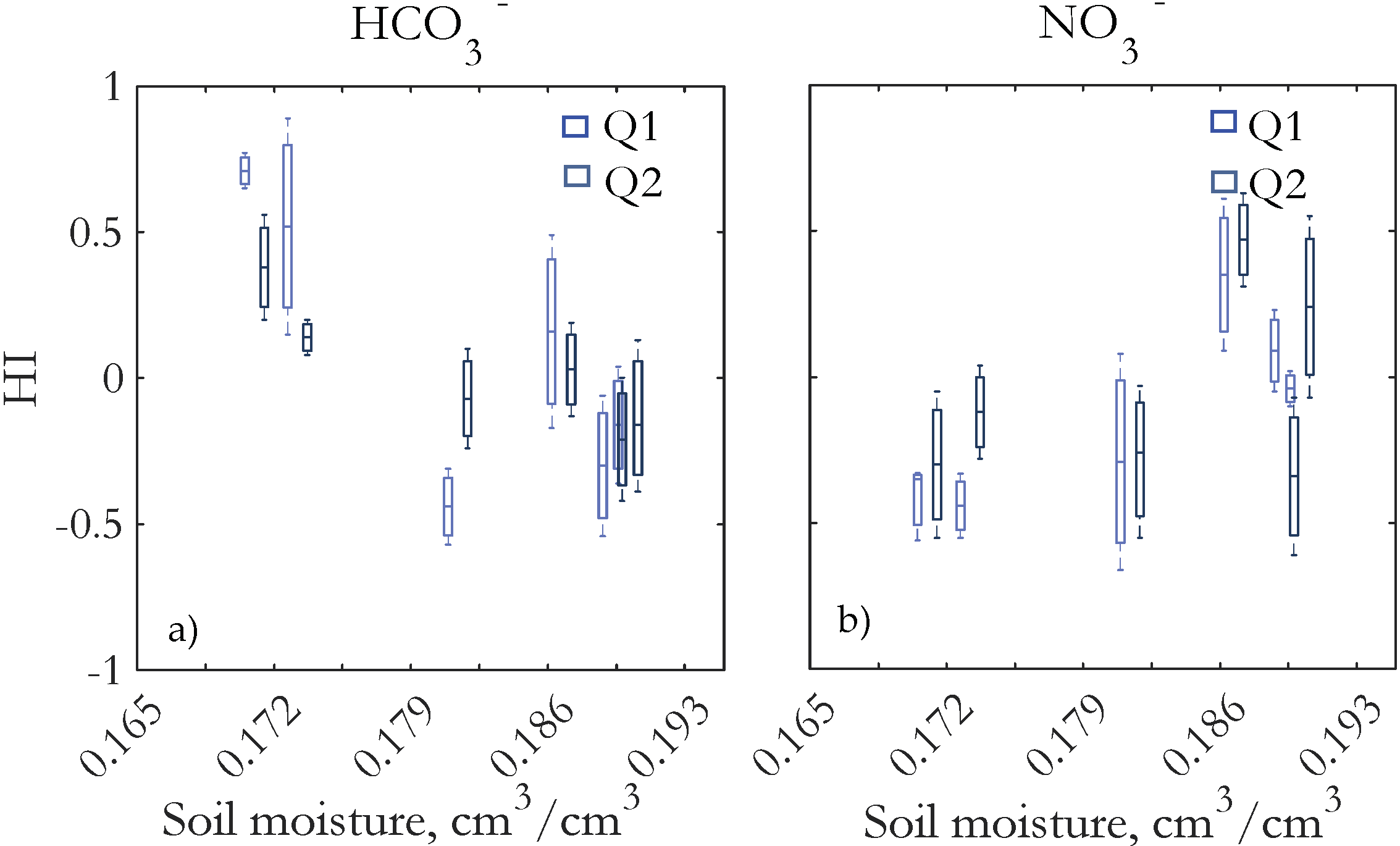
3.5. Soil Moisture and Hysteresis Index (HI) Relationship

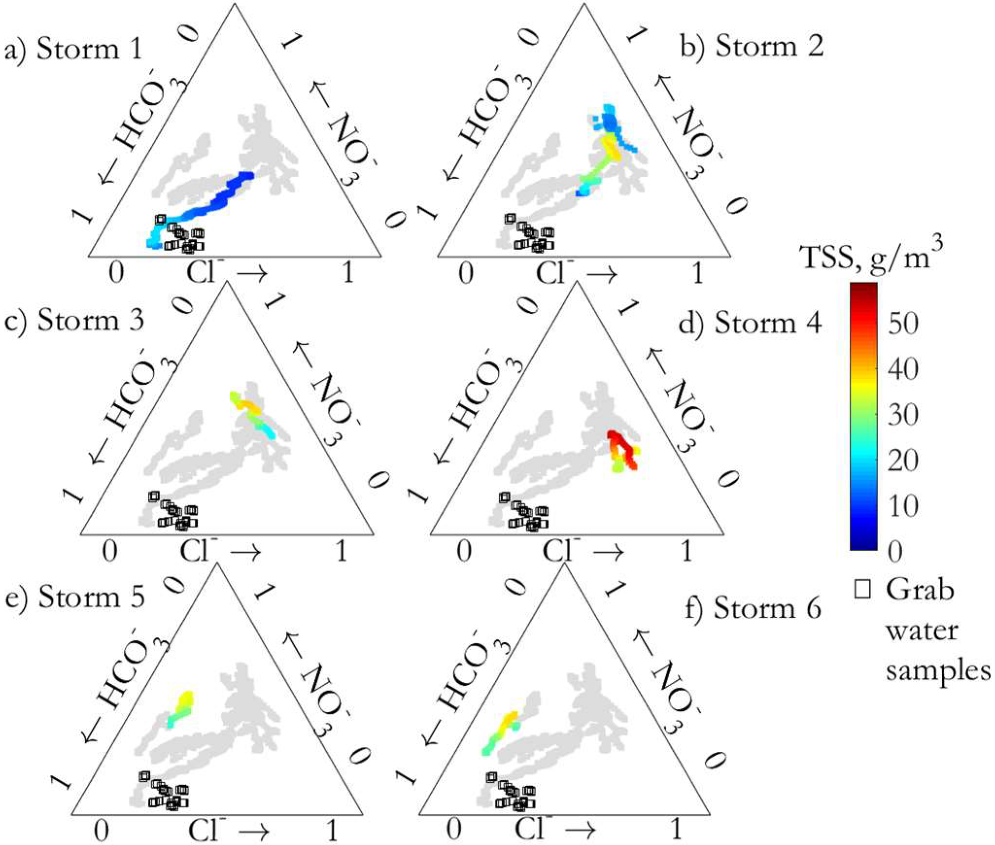
Concentrations of ions in the river are highly influenced by the catchment conditions [44]. However, the transport of ions is highly dependent on the precipitation regime that wets the catchment and causes surface runoff [45], which in turn is driven by the slope and land use/land cover [46]. To know the relationship between rainstorms and catchment wetness conditions, this study also assessed each rainstorm using the estimated soil moisture and the ionic mobilization by means of the HI in the six rainstorms (Figure 6). The soil moisture for each rainstorm was correlated with HI. It was found that the HI of HCO₃⁻ (Figure 6a) increased as the soil moisture decreased, whereas the HI of NO₃⁻ decreased as soil moisture decreased (Figure 6b). Such a relationship implied the influence of soil moisture in the hysteresis loop direction [47]. It should be noted also that the HI discrepancy between Q1 and Q2 for HCO₃⁻ and NO₃⁻ was the result of disturbances caused by contributions of point and nonpoint sources of pollutants added to the river in the drainage area shaped between these two locations.

3.6. Anions and TSS

To illustrate changes of anions simultaneously during rainstorms, Figure 7 depicts the anions diagram for location Q1, which was built by replacing SO₄²⁻ with NO₃⁻ with the aim to consider nutrient load effects in the catchment. It was found that grab water samples and continuous monitoring had different zones within the anions diagram. In addition, it was identified that rainstorms induced changes in concentrations of HCO₃⁻, NO₃⁻ and Cl⁻, which evolved differently for each rainstorm, defining a region for rainstorms 1–4 that was reduced in rainstorms 5 and 6.

Anions concentrations were the consequence of mobilization in the catchment and along the river, which are often influenced by anthropogenic activities driving contamination [48]. These ion concentrations varied based on catchment wetness conditions at the onset of each rainstorm, which can be defined by the soil moisture due to the antecedent precipitation. For instance, the transient response of anions in rainstorms 1 and 2 (Figure 7a,b) significantly differed when compared to rainstorms 5 and 6 (Figure 7e–f), where soil moisture increased from 0.17 to 0.18 cm³/cm³.

On the other hand, estimations of TSS were possible with the power-law equation. TSS relied on the flow q with coefficients a and b. Calibration (R² = 0.67) for Q2 (Figure S2) resulted in Equation (5), which had a higher coefficient of determination than relying on turbidity measurements.

$$TSS\left(q\right)=0.4747q^{0.6195}$$

(5)

Then, TSS were also added in Figure 7 as part of the transient response of anionic concentration of each rainstorm. The variability of TSS during rainstorms was driven by flow q. It was evident that low (Figure 7a) and high (Figure 7d) values of TSS were led by low and high flow q in rainstorms 1 and 4, respectively, and any rainstorm had a peak flow q which induced the maximum TSS (Table S2).

TSS changes during rainstorms were also driven by the effects of anthropogenic activities [49]. Anthropogenic activities may cause physical scouring of river banks and beds and erosion of adjacent soil when compared to native land use and vegetation [46]. This causes TSS to have mobilization at the same time as ions (Figure S3) along the river.

Nonetheless, the transport of anions and TSS in the river will respond at a different pace during the time of a rainstorm [36]. For instance, rainstorms 1 and 2 (Figure 7a,b) had an increase in flow q that induced a simultaneous response in TSS and anions. These simultaneous responses varied during consecutive rainstorms 3–6 (Figure 7c–f). The reason for a particular response for each anion could be associated with river processes such as aquatic photosynthesis that reduces nitrates [50] and dissolved carbon dioxide, and it also induces changes of pH and carbonaceous compounds [51]. In this way, the TSS and anions may need specific adjustments beyond the flow due to several factors related with the catchment such as antecedent precipitation and its spatial distribution (Figure S1).

4. Conclusions

Investigation of the Kanawha River as a mainstream of the Central Appalachia Region allowed us to identify the river water chemistry and its potential disruption caused by rainstorms observed during the winter. It was also possible to know the influence of catchment wetness conditions through soil moisture and its impact on rainstorms through the c–q relationship. This study represented an effort to merge hydrology, hydrodynamics and water chemistry using grab water samples and high-frequency data. It was revealed that the distributions of cations were as follows: Ca²⁺ (55%) > Mg²⁺ (20%) > Na⁺ (18%) > K⁺ (7%), and anions: SO₄²⁻ (62%) > HCO₃⁻ (22%) > Cl⁻ + NO₃⁻ (16%). The type of water was classified mostly as Ca²⁺ -Cl⁻, according to the Piper diagram. The origin of dissolved solids was mainly derived from rock weathering based on the Gibbs diagram. Within this context, concentrations of HCO₃⁻, Cl⁻ and NO₃⁻ were investigated in conjunction with TSS during rainstorms. It was found that the application of hysteresis to c–q for HCO₃⁻ had consistent loop directions between Q1 and Q2 for the six rainstorms. In contrast, the c–q for NO₃⁻ had a consistent loop direction between Q1 and Q2 only for rainstorms 1–4. NO₃⁻ had reached maximum dilution and depended on local discharges for rainstorms 5 and 6, causing an opposed loop direction between Q1 and Q2. In addition to the hysteretic effect based on the locations along the river, it was also found that the soil moisture was a crucial factor influencing the magnitude of HI for HCO₃⁻ and NO₃⁻.

These findings further help to improve our understanding of sediment and river water chemistry conditions that ultimately affect aquatic biota. The integration of hydrologic and river processes will lead to the development of comprehensive c–q relationships and will better explain how river water chemistry conditions are reset.

References

1. Qin, C.; Li, S.L.; Waldron, S.; Yue, F.J.; Wang, Z.J.; Zhong, J.; Ding, H.; Liu, C.Q. High-frequency monitoring reveals how hydrochemistry and dissolved carbon respond to rainstorms at a karstic critical zone, Southwestern China. Sci. Total Environ. 2020, 714, 136833. [Google Scholar] [CrossRef] [PubMed]
2. Palmer, M.; Ruhi, A. Linkages between flow regime, biota, and ecosystem processes: Implications for river restoration. Science 2019, 365, eaaw2087. [Google Scholar] [CrossRef] [PubMed]
3. Burns, D.A.; Pellerin, B.A.; Miller, M.P.; Capel, P.D.; Tesoriero, A.J.; Duncan, J.M. Monitoring the riverine pulse: Applying high-frequency nitrate data to advance integrative understanding of biogeochemical and hydrological processes. Wiley Interdiscip. Rev. Water 2019, 6, e1348. [Google Scholar] [CrossRef]
4. Griffith, M.B.; Norton, S.B.; Alexander, L.C.; Pollard, A.I.; LeDuc, S.D. The effects of mountaintop mines and valley fills on the physicochemical quality of stream ecosystems in the central Appalachians: A review. Sci. Total Environ. 2012, 417–418, 1–12. [Google Scholar] [CrossRef] [PubMed]
5. Mari, I.; Myron, J.M.; Charles, T.D. Spatial patterns of precipitation quantity and chemistry and air temperatures in the Adirondack region of New York. Atmos. Environ. 2002, 36, 1051–1062. [Google Scholar]
6. Anderson, J.B.; Baumgardner, R.E.; Mohnen, V.A.; Bowser, J.J. Cloud chemistry in the eastern United States, as sampled from three high-elevation sites along the Appalachian Mountains. Atmos. Environ. 1999, 33, 5105–5114. [Google Scholar] [CrossRef]
7. Butler, B.A.; Ford, R.G. Evaluating relationships between total dissolved solids (TDS) and total suspended solids (TSS) in a mining-influenced watershed. Mine Water Environ. 2018, 37, 18–30. [Google Scholar] [CrossRef]
8. Aguilera, R.; Melack, J.M. Concentration-Discharge Responses to Storm Events in Coastal California Watersheds. Water Resour. Res. 2018, 54, 407–424. [Google Scholar] [CrossRef]
9. Musolff, A.; Schmidt, C.; Selle, B.; Fleckenstein, J.H. Catchment controls on solute export. Adv. Water Resour. 2015, 86, 133–146. [Google Scholar] [CrossRef]
10. Jonnalagadda, S.B.; Mhere, G. Water quality of the odzi river in the Eastern Highlands of Zimbabwe. Water Res. 2001, 35, 2371–2376. [Google Scholar] [CrossRef]
11. Piper, A.M. A graphic procedure in the geochemical interpretation of water-analyses. Eos Trans. Am. Geophys. Union 1944, 25, 914–928. [Google Scholar] [CrossRef]
12. Gibbs, R.J. Mechanisms Controlling World Water Chemistry. Science 1970, 170, 1088–1090. [Google Scholar] [CrossRef] [PubMed]
13. Moatar, F.; Abbott, B.W.; Minaudo, C.; Curie, F.; Pinay, G. Elemental properties, hydrology, and biology interact to shape concentration-discharge curves for carbon, nutrients, sediment, and major ions. Water Resour. Res. 2017, 53, 1270–1287. [Google Scholar] [CrossRef]
14. Rose, L.A.; Karwan, D.L.; Godsey, S.E. Concentration–discharge relationships describe solute and sediment mobilization, reaction, and transport at event and longer timescales. Hydrol. Process. 2018, 32, 2829–2844. [Google Scholar] [CrossRef]
15. Knapp, J.L.A.; von Freyberg, J.; Studer, B.; Kiewiet, L.; Kirchner, J.W. Concentration-discharge relationships vary among hydrological events, reflecting differences in event characteristics. Hydrol. Earth Syst. Sci. 2020, 24, 2561–2576. [Google Scholar] [CrossRef]
16. Rozemeijer, J.C.; Van Der Velde, Y.; Van Geer, F.C.; De Rooij, G.H.; Torfs, P.J.J.F.; Broers, H.P. Improving load estimates for NO3 and P in surface waters by characterizing the concentration response to rainfall events. Environ. Sci. Technol. 2010, 44, 6305–6312. [Google Scholar] [CrossRef]
17. Beaudoing, H.; Rodell, M. GLDAS Noah Land Surface Model L4 3 Hourly 0.25 × 0.25 Degree V2.0; Goddard Earth Sciences Data and Information Services Center (GES DISC): Greenbelt, MD, USA, 2020. [Google Scholar]
18. Beaudoing, H.; Rodell, M. GLDAS Noah Land Surface Model L4 3 Hourly 0.25 × 0.25 Degree V2.1; Goddard Earth Sciences Data and Information Services Center (GES DISC): Greenbelt, MD, USA, 2020. [Google Scholar]
19. Fedora, M.A.; Beschta, R.L. Storm runoff simulation using an antecedent precipitation index (API) model. J. Hydrol. 1989, 112, 121–133. [Google Scholar] [CrossRef]
20. Petty, J.T.; Fulton, J.B.; Strager, M.P.; Merovich, G.T.; Stiles, J.M.; Ziemkiewicz, P.F. Landscape indicators and thresholds of stream ecological impairment in an intensively mined Appalachian watershed. J. N. Am. Benthol. Soc. 2010, 29, 1292–1309. [Google Scholar] [CrossRef]
21. Evans, C.; Davies, T.D. Causes of concentration/discharge hysteresis and its potential as a tool for analysis of episode hydrochemistry. Water Resour. Res. 1998, 34, 129–137. [Google Scholar] [CrossRef]
22. Orndorff, Z.W.; Daniels, W.L.; Zipper, C.E.; Eick, M.; Beck, M. A column evaluation of Appalachian coal mine spoils’ temporal leaching behavior. Environ. Pollut. 2015, 204, 39–47. [Google Scholar] [CrossRef]
23. Rojano, F.; Huber, D.H.; Ugwuanyi, I.R.; Lhilhi Noundou, V.; Kemajou-Tchamba, A.L.; Chavarria-Palma, J.E. Net Ecosystem Production of a River Relying on Hydrology, Hydrodynamics and Water Quality Monitoring Stations. Water 2020, 12, 783. [Google Scholar] [CrossRef] [Green Version]
24. U.S. Geological Survey (USGS). National Water Information System Data (NWIS). Available online: http://waterdata.usgs.gov/nwis/ (accessed on 22 February 2022).
25. Muti-Resolution Land Characteristics (MRLC). National Land Cover Database (NLCD). Available online: https://www.mrlc.gov/ (accessed on 1 November 2021).
26. Natural Resources Conservation Service (NRCS). United States Department of Agriculture, (USDA). Web Soil Survey, (WSS). Available online: https://websoilsurvey.sc.egov.usda.gov (accessed on 23 January 2022).
27. WV Geology West Virginia Geological and Economic Survey (WVGES). Available online: http://www.wvgs.wvnet.edu (accessed on 28 July 2020).
28. Schulte, P.; van Geldern, R.; Freitag, H.; Karim, A.; Négrel, P.; Petelet-Giraud, E.; Probst, A.; Probst, J.L.; Telmer, K.; Veizer, J.; et al. Applications of stable water and carbon isotopes in watershed research: Weathering, carbon cycling, and water balances. Earth-Sci. Rev. 2011, 109, 20–31. [Google Scholar] [CrossRef]
29. Lewis, E.R.; Wallace, D.W.R. Program Developed for CO2 System Calculations, ORNL/CDIAC-105; Carbon Dioxide Information Analysis Center (CDIAC), Oak Ridge National Laboratory: Oak Ridge, TN, USA, 1998. [Google Scholar]
30. Liu, S.; Raymond, P.A. Hydrologic controls on pCO2 and CO2 efflux in US streams and rivers. Limnol. Oceanogr. Lett. 2018, 3, 428–435. [Google Scholar] [CrossRef]
31. Ran, L.; Lu, X.X.; Liu, S. Dynamics of riverine CO2 in the Yangtze River fluvial network and their implications for carbon evasion. Biogeosciences 2017, 14, 2183–2198. [Google Scholar] [CrossRef]
32. Li, S.; Luo, J.; Wu, D.; Jun Xu, Y. Carbon and nutrients as indictors of daily fluctuations of pCO2 and CO2 flux in a river draining a rapidly urbanizing area. Ecol. Indic. 2020, 109, 105821. [Google Scholar] [CrossRef]
33. Hotchkiss, E.R.; Hall, R.O.; Sponseller, R.A.; Butman, D.; Klaminder, J.; Laudon, H.; Rosvall, M.; Karlsson, J. Sources of and processes controlling CO2emissions change with the size of streams and rivers. Nat. Geosci. 2015, 8, 696–699. [Google Scholar] [CrossRef]
34. National Aeronautics and Space Administration (NASA). Global Land Data Assimilation System (GLDAS). Catchment Land Surface Model (CLSM). Available online: https://giovanni.gsfc.nasa.gov (accessed on 14 July 2022).
35. Knapp, J.L.A.; Osenbrück, K.; Brennwald, M.S.; Cirpka, O.A. In-situ mass spectrometry improves the estimation of stream reaeration from gas-tracer tests. Sci. Total Environ. 2019, 655, 1062–1070. [Google Scholar] [CrossRef]
36. Moatar, F.; Floury, M.; Gold, A.J.; Meybeck, M.; Renard, B.; Ferréol, M.; Chandesris, A.; Minaudo, C.; Addy, K.; Piffady, J.; et al. Stream Solutes and Particulates Export Regimes: A New Framework to Optimize Their Monitoring. Front. Ecol. Evol. 2020, 7, 516. [Google Scholar] [CrossRef]
37. Lloyd, C.E.M.; Freer, J.E.; Johnes, P.J.; Collins, A.L. Technical Note: Testing an improved index for analysing storm discharge-concentration hysteresis. Hydrol. Earth Syst. Sci. 2016, 20, 625–632. [Google Scholar] [CrossRef]
38. Eder, A.; Strauss, P.; Krueger, T.; Quinton, J.N. Comparative calculation of suspended sediment loads with respect to hysteresis effects (in the Petzenkirchen catchment, Austria). J. Hydrol. 2010, 389, 168–176. [Google Scholar] [CrossRef]
39. 2540 Solids; Standard Methods for the Examination of Water and Wastewater. Lipps, W.C.; Baxter, T.E.; Braun-Howland, E. (Eds.) American Public Health Association Press: Washington, DC, USA, 2017.
40. Huffman, G.J.; Bolvin, D.T.; Nelkin, E.J.; Adler, R.F. TRMM (TMPA) Precipitation L3 1 Day 0.25 Degree × 0.25 Degree V7; Savtchenko, A., Ed.; Goddard Earth Sciences Data and Information Services Center (GES DISC): Greenbelt, MD, USA, 2020. [Google Scholar]
41. Ludwikowski, J.J.; Peterson, E.W. Transport and fate of chloride from road salt within a mixed urban and agricultural watershed in Illinois (USA): Assessing the influence of chloride application rates. Hydrogeol. J. 2018, 26, 1123–1135. [Google Scholar] [CrossRef]
42. Haake, D.M.; Knouft, J.H. Comparison of Contributions to Chloride in Urban Stormwater from Winter Brine and Rock Salt Application. Environ. Sci. Technol. 2019, 53, 11888–11895. [Google Scholar] [CrossRef] [PubMed]
43. Misset, C.; Recking, A.; Legout, C.; Poirel, A.; Cazilhac, M.; Esteves, M.; Bertrand, M. An attempt to link suspended load hysteresis patterns and sediment sources configuration in alpine catchments. J. Hydrol. 2019, 576, 72–84. [Google Scholar] [CrossRef]
44. Lechuga-Crespo, J.L.; Ruiz-Romera, E.; Probst, J.L.; Unda-Calvo, J.; Cuervo-Fuentes, Z.C.; Sánchez-Pérez, J.M. Combining punctual and high frequency data for the spatiotemporal assessment of main geochemical processes and dissolved exports in an urban river catchment. Sci. Total Environ. 2020, 727, 138644. [Google Scholar] [CrossRef] [PubMed]
45. Camacho Suarez, V.V.; Saraiva Okello, A.M.L.; Wenninger, J.W.; Uhlenbrook, S. Understanding runoff processes in a semi-arid environment through isotope and hydrochemical hydrograph separations. Hydrol. Earth Syst. Sci. 2015, 19, 4183–4199. [Google Scholar] [CrossRef]
46. Koskelo, A.I.; Fisher, T.R.; Sutton, A.J.; Gustafson, A.B. Biogeochemical storm response in agricultural watersheds of the Choptank River Basin, Delmarva Peninsula, USA. Biogeochemistry 2018, 139, 215–239. [Google Scholar] [CrossRef]
47. Baker, E.B.; Showers, W.J. Hysteresis analysis of nitrate dynamics in the Neuse River, NC. Sci. Total Environ. 2019, 652, 889–899. [Google Scholar] [CrossRef]
48. Ustaoğlu, F.; Tepe, Y. Water quality and sediment contamination assessment of Pazarsuyu Stream, Turkey using multivariate statistical methods and pollution indicators. Int. Soil Water Conserv. Res. 2019, 7, 47–56. [Google Scholar] [CrossRef]
49. Stets, E.G.; Sprague, L.A.; Oelsner, G.P.; Johnson, H.M.; Murphy, J.C.; Ryberg, K.; Vecchia, A.V.; Zuellig, R.E.; Falcone, J.A.; Riskin, M.L. Landscape Drivers of Dynamic Change in Water Quality of U.S. Rivers. Environ. Sci. Technol. 2020, 54, 4336–4343. [Google Scholar] [CrossRef]
50. Marescaux, A.; Thieu, V.; Borges, A.V.; Garnier, J. Seasonal and spatial variability of the partial pressure of carbon dioxide in the human-impacted Seine River in France. Sci. Rep. 2018, 8, 13961. [Google Scholar] [CrossRef]
51. Ran, L.; Lu, X.X.; Richey, J.E.; Sun, H.; Han, J.; Yu, R.; Liao, S.; Yi, Q. Long-term spatial and temporal variation of CO2 partial pressure in the Yellow River, China. Biogeosciences 2015, 12, 921–932. [Google Scholar] [CrossRef] [Green Version]
Figure 1. Catchment area of the Kanawha River, West Virginia, indicating location of flow gages and water quality monitoring stations.
Water 14 02687 g001
Figure 2. Piper diagram to characterize water chemistry of the Kanawha River using 45 water samples collected during 2016–2018 (further information in Table S1).
Water 14 02687 g002
Figure 3. Gibbs diagram relating total dissolved solids (TDS) to (a) cations Na+/(Na+ + Ca2+) and (b) anions Cl/(Cl + HCO3) for the Kanawha River using 45 water samples collected during 2016-2018 (further information in Table S1).
Water 14 02687 g003
Figure 4. Time series area-averaged of precipitation (a,f in location Q1 and Q2, respectively) were not immediately reflected in the increase in flow (b) due to the scale of the catchment; rather, the increase in flow was a consequence of the combined precipitation observed at drainage areas Q1 and Q2. Estimated soil moisture (c), water temperature (g), NO3 (d), pH (e), turbidity (h) and Cl (i), and HCO3 (j) with Q1 and Q2 locations along the Kanawha River indicated in Figure 1.
Water 14 02687 g004
Figure 5. Hysteresis of six rainstorms using HCO3 (af), NO3 (gl) and Cl (mr) in Q1 and Q2 locations along the Kanawha River. The transient response advances in Q1 and Q2 from 0 to 1 for any rainstorm.
Water 14 02687 g005
Figure 6. Relationships of the (a) HCO3 and (b) NO3 between soil moisture and hysteresis index (HI) for Q1 and Q2 locations along the Kanawha River indicated in Figure 1.
Water 14 02687 g006
Figure 7. Anions diagram of HCO3, NO3 and Cl during six rainstorms (af) in conjunction with total suspended sediments (TSS) and grab water samples (☐) for location Q1 in the Kanawha River, West Virginia (gray footprint corresponds to all measurements of Figure 4).
Water 14 02687 g007