Effects of Microtopography on Runoff Generation in Plain Farmland: New Insights from an Event-Based Rainfall–Runoff Model

Abstract

Plain farmland areas without significant topographic slope exhibit microtopographic features of different scales. Quantitative assessment of the effects of microtopography at different scales on runoff generation in typical farmland areas is of great significance for regional water resources management and flood disaster forecasting. The main objective of the study was to develop an event-based rainfall–runoff model based on the layered Green–Ampt model (LGAM) with the consideration of plot-scale microtopographic features in plain farmland areas. Our experimental field, located in Taihu Lake Basin, was classified into three types of topographic subunits (i.e., main field, rill, and ditch) according to the average elevation. To simplify the concentration process for three topographic subunits, the average concentration time method was employed. Here, various experimental scenarios were simulated, including two classical unsteady rainfall events in homogeneous soil, one ponding infiltration experiment, and two typical rainfall–runoff events in the experimental field. We found that the multilayered setting showed higher accuracy than the homogeneous setting for simulating infiltration in the ponding infiltration experiment in the field. The RMSE of simulated ponding water depth reduced from 0.166 cm to 0.035 cm and NSE rose from 0.988 to 0.999. The simulated hydrograph considering microtopography effects proved higher accuracy than that under unified topography assumption. After classifying topography, the RMSE and NSE of simulated hydrographs decreased and increased, respectively. The lower the topographic subunit, the earlier the outflow occurred. At the early stage, the runoff mostly originated from the relatively low topographic subunits. Infiltration-excess regime under saturated condition may initially dominate in the low-lying ditch under intense rainfall, with extremely high runoff coefficient. Concentration process in the plain farmland area was affected by both rainfall intensity and microtopography. The greater the rainfall intensity, the shorter the average concentration time. The concentration velocity under heavy rainfall was four times faster than that under light rainfall. The lower topographic subunit was characterized by shorter concentration pathway and average concentration time. Ditches reduced the peak flow and advanced the time to peak. This quantitative study provides new insights into effects of microtopography on runoff generation in plain farmland area as well as an effective alternative for plot-scale rainfall–runoff modeling.

1. Introduction

In plain farmland areas, surface runoff is an important process that affects the local water balance and causes soil erosion and rapid solute transport [1,2]. It occurs ephemerally as sheet flow and channel flow in microchannels [3]. As the topographic gradients of plain farmland areas can be negligible, microtopography becomes the essential element of farmland field landscape.

There have been various definitions of ‘microtopography’ in previous studies. Thompson [4] defined microtopography as millimeter to centimeter scales while Frei [5] thought of it in larger scales (i.e., centimeters to meters). Chu [6] characterized surface microtopography by depressions/pits/puddles, mounds/peaks, ridges, and channels, which covered a wide scale range. Apples called these topographic features meso- and microtopography [7]. In this paper, we define ‘microtopography’ as centimeter to meter scale, including many (ir)regular topographical features, such as surface depressions [8], rills [9,10], and small drainage ditches [11,12]. These topographical features are usually induced by tillage [13] or rainfall–runoff erosion [14].

Microtopographic characteristics have evident effects on surface connectivity [15], infiltration volume [4,7], depression storage [13,16,17], runoff [18,19,20], concentration processes [5,8,21,22], and even biogeochemical process activities [23]. Accordingly, microtopography is one of the critical factors that influence runoff generation processes in plain farmland.

Several model-based studies have addressed the effect of different microtopography scales on runoff dynamics. Some models were developed to quantify hydrological connectivity of surface depressions at field scale [2,7,8,24,25], in which the puddle-to-puddle (P2P) conceptual model [8,25] can simulate the entire hierarchical drainage network accounting for surface depressions within an overland flow system. Additionally, other models were developed considering the specific effect of rills [26,27] or drainage ditches [28,29,30,31]. However, few models have been used to quantify the effects of microtopography at different scales on runoff generation in farmland areas.

Theoretically, Integrated Surface–Subsurface Hydrological Models (ISSHMs) can quantify the effects of microtopography at different scales on runoff generation in plain farmland areas. Frei [18] built a model in the HydroGeoSphereto explore the feedback among groundwater levels, ponding, and surface runoff in a riparian wetland with a heterogeneous microtopography. Nevertheless, such a complex model requires high grid resolutions to capture relevant small-scale variations in topography at the range of centimeters to meters [32]. High grid resolutions usually result in longer simulation times, especially if fully integrated model approaches are used where the governing partial differential equations for surface and subsurface flow are solved simultaneously [33]. To reduce computational nodes while preserving important effects of microtopography on surface flow generation and subsurface transport characteristics, Frei replaced the explicit microtopography with spatially distributed rill/depression storage zones [5]. Even so, such a framework is still too complex for plot-scale modeling.

Event-based models merely require data at the event scale and are easy to calibrate [34], which are very suitable for runoff generation regime study [35,36,37]. An agricultural plot with microtopography at different scales (i.e., surface depressions, rills, and small ditches) can be considered as the smallest response unit in farmed landscapes [28,38]. Therefore, an effective alternative for plot-scale rainfall–runoff modeling that considers effects of surface microtopography at different scales in plain farmland is necessary.

In this study, a typical plain farmland field in Taihu Lake Basin plain was classified into three kinds of topographic subunits. Two typical rainfall patterns in the experimental field were selected to simulate, i.e., short-duration rainstorm and long-duration light rainfall. The objectives of this study are (1) to propose a simple and effective event-based rainfall–runoff model considering effects of surface microtopography at different scales for plain farmland and (2) to evaluate the difference of spatial contribution rates of runoff in different rainfall patterns. In this paper, the field experiments and the model structure are provided in Section 2. The modeling results for typical cases are presented in Section 3. Several significant points are discussed in Section 4. Conclusions are made in Section 5.

2. Materials and Methods

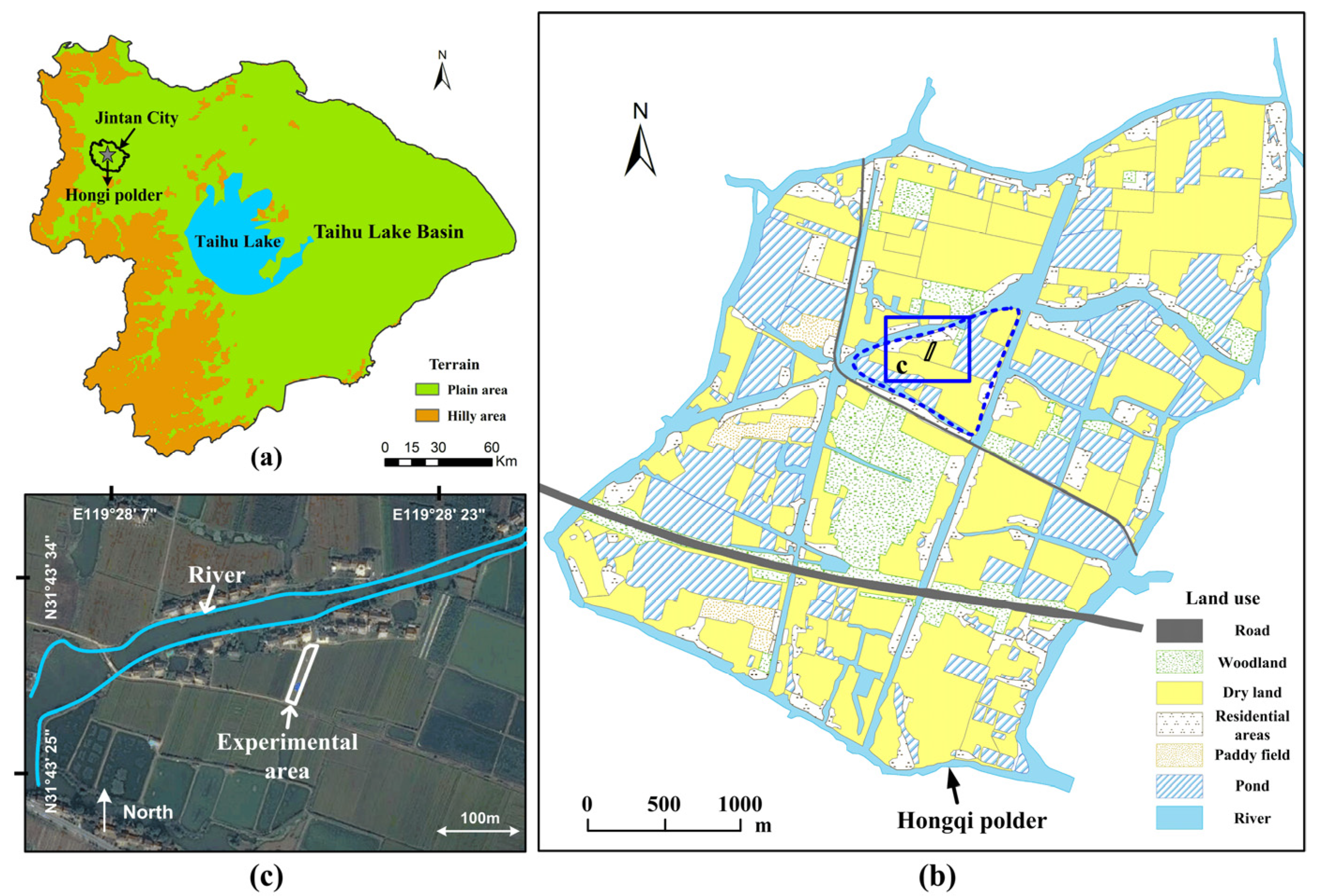
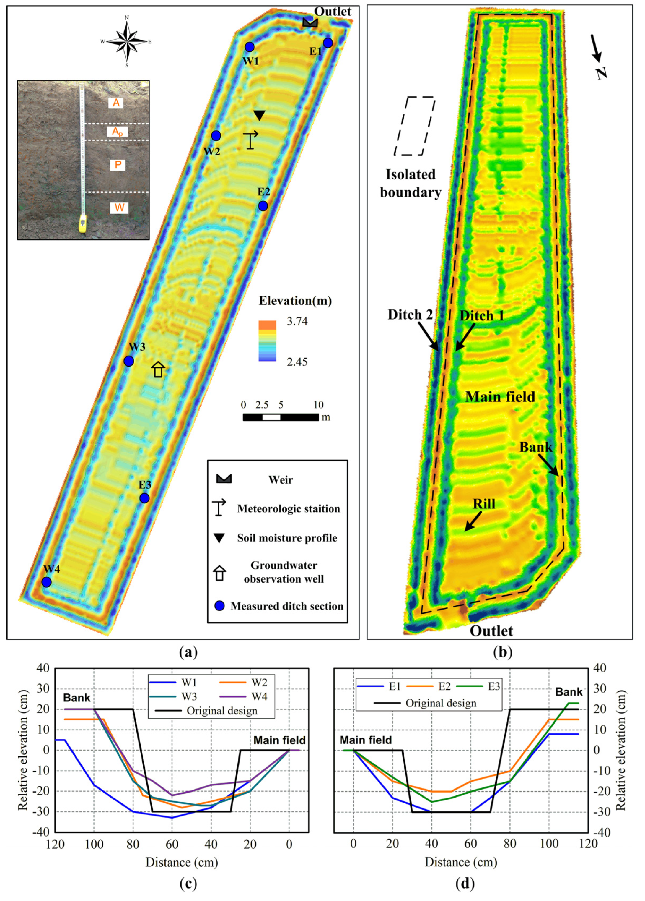
2.1. Site, Instrument, and Soil Sampling

The study site is located in Hongqi polder, Jintan County in Taihu Lake Basin (Figure 1a), which is characterized by a large number of plain farmlands. The region has a subtropical monsoon climate with 723–1836 mm annual rainfall and 1041–1562 mm annual mean potential evaporation. The landscape mainly consists of dry land and woodland interspersed by rivers and ponds (Figure 1b). The selected area (N 31°43′30″, E 119°28′15″, Figure 1c) was initially a rice–wheat rotation field that was converted into dry land in 2011. The annual average phreatic water table depth is about 0.6 m. Soybean is planted from July to September and oilseed rape is planted from November to May of the next year. A previous study has shown that the variation of soil water content at this experimental field is dependent on the comprehensive influence of soil hydraulic properties, meteorological factors, and shallow groundwater [39]. Furthermore, Dunne overland flow was the dominant mechanism responsible for the rapid runoff generation in this area due to shallow groundwater [40].

The area of the field is 1008 m², in which 4186 scattered elevation sample points were collected. The average sampling density was about 4 points/m² and the corresponding sampling interval was 0.5 m. We adopted the Regularized Spline interpolation method to obtain 0.1 m-resolution DEM of the field (Figure 2a). The elevations varied from 2.45 m to 3.74 m with a mean of 3.14 m. Distinct layered characteristics can be seen from the excavated soil profile in the field, i.e., 0–13 cm is plough layer(A), 13–22 cm is plow pan (A_p), 22–47 cm is percogenic horizon(P), and below 47 cm is waterloggogenic horizon(W). A meteorological station, a soil moisture profile (10 cm, 20 cm, 40 cm, 60 cm, 80 cm, 100 cm), and a groundwater observation well has been set up in the field since 2011.

The experimental field is surrounded by narrow banks to obstruct water. In order to minimize the lateral leakage from banks, a waterproof barrier (1.5 m-depth) was inserted into banks (Figure 2b). The contributing area inside the isolated boundary is about 912 m² with an average length of 87 m and average width of 10.5m. Meanwhile, Ditch 1 and Ditch 2 are the two main artificial drainage pathways surrounding the main field. Ditch 1 collects the outflow from the main field and Ditch 2 collects the lateral leakage flow from rice fields outside. A 90° V-notch weir was set up to measure outflow discharge at the outlet of Ditch 1.

The original size of the inner ditch section was trapezoidal with an upper width of 70 cm, a lower width of 40 cm, and a depth varying from 30 to 40 cm. However, due to the rainfall erosion and runoff scouring for many years, the shape of the section gradually changes. We measured seven sections of Ditch 1 in May 2017 and found that the bottom of the ditch was 20–30 cm lower than the main field (Figure 2c,d).

Soil samples were collected at 0–10 cm, 10–20 cm, 20–40 cm, 40–60 cm, and 60–80 cm depths in three profiles in the field. Grain composition, physical properties, and saturated hydraulic conductivities were measured (

Table 1. Average values of grain composition, physical properties, and saturated hydraulic conductivities of five depths in the experimental field. Range is in parentheses (minimum/maximum values).

Depth (cm)	Clay (-)	Silt (-)	${\mathit{\rho }}_{\mathit{b}}$ (g/cm3)	$\mathit{n}$ (-)	Ks (cm/min)
0–10 10–20 20–40 40–60 60–80	0.31 (0.27–0.34) 0.29 (0.26–0.34) 0.29 (0.26–0.32) 0.33 (0.30–0.35) 0.41 (0.38–0.43)	0.57 (0.53–0.62) 0.61 (0.58–0.64) 0.63 (0.61–0.67) 0.61 (0.58–0.64) 0.54 (0.53–0.58)	1.20 (1.10–1.28) 1.23 (1.05–1.50) 1.47 (1.41–1.50) 1.46 (1.35–1.53) 1.46 (1.41–1.50)	0.55(0.52–0.58) 0.50(0.43–0.60) 0.45(0.43–0.47) 0.45(0.42–0.49) 0.45(0.42–0.47)	0.07(0.02–0.25) 0.08(0.01–0.22) 0.07(0.02–0.13) 0.11(0.04–0.18) 0.03(0.01–0.05)

). The soil above 60 cm is silty clay loam, while the soil below 60 cm changes to silty clay. The dry bulk density (${\rho }_b$) gradually increases with depth while the average porosity ($n$) decreases with depth. The dry bulk densities of the soil below 20 cm are basically the same and much larger than those of the upper soil. The average porosities of 0–10 cm and 10–20 cm are 0.55 and 0.50, respectively. The average porosities of 20–80 cm decrease to 45%. The average saturated hydraulic conductivity of 60–80 cm is much less than those of upper layers.

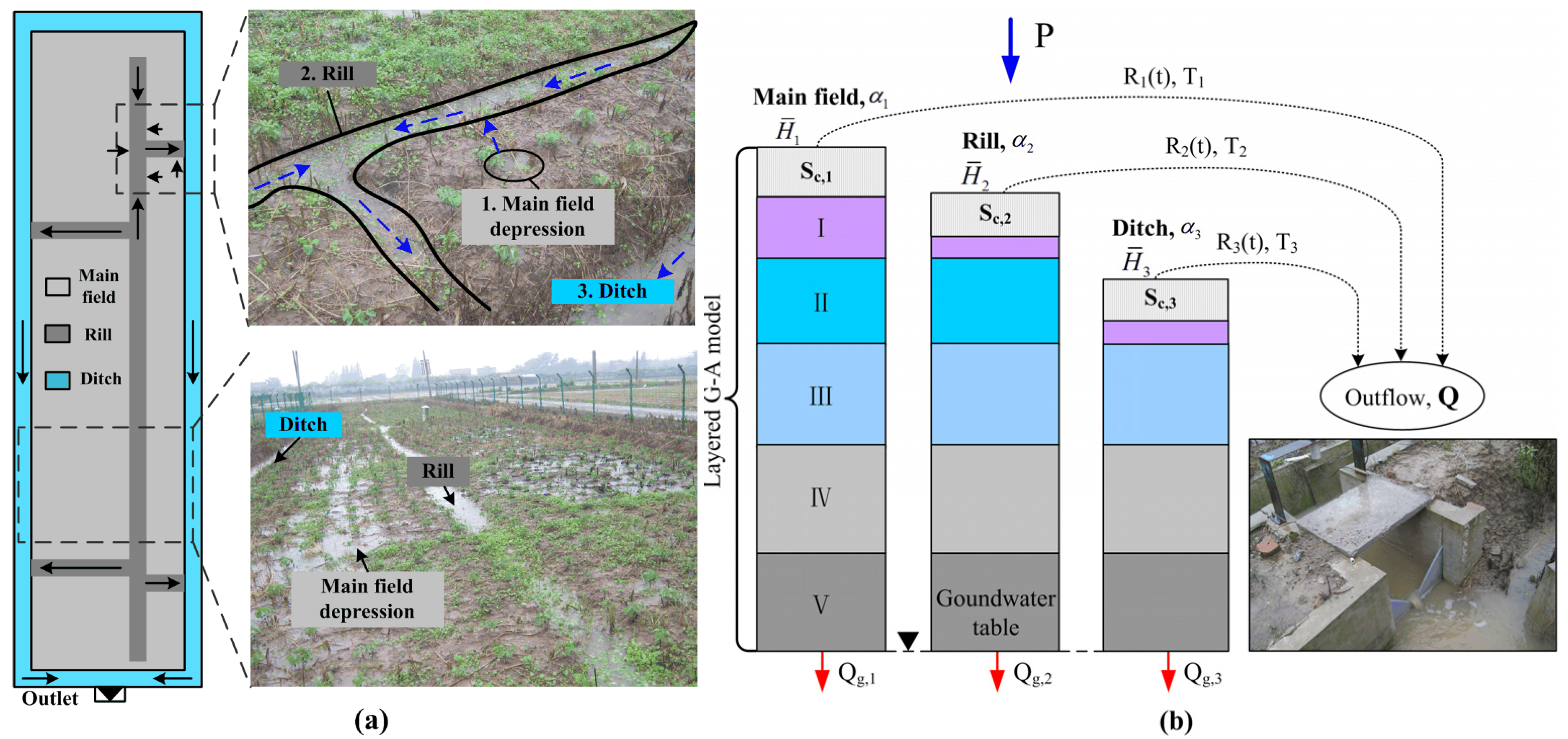
2.2. Model Structure

The Green–Ampt(G–A) model [41] is a simplified representation of the infiltration process, which has been widely used in hydrology. Some modified version of the Green–Ampt model has been widely used for simulating infiltration and rainfall–runoff processes [42]. After long-term farming and sedimentation, farmland soils present structured and stratified layers [43,44], which may greatly change the soil physical as well as hydraulic properties [45,46]. The layered Green–Ampt model(LGAM) proposed by Liu [47] considered the layered characteristics of soil and calculated ponding time, outflow time, and water budget composition accurately. We modified this LGAM as the runoff generation module.

The module structure can be seen in Figure 3, in which UZT is unsaturated zone thickness, $N$ is the number of unsaturated soil layers, $D_i$ is thickness of each unsaturated layer, WFD is wetting front depth, ${\theta }_{i,0}$ is initial soil water content of ith layer, and ${\theta }_{i,s}$ is saturated soil water content of ith layer. As the surface depressions can store a certain amount of excess water on the soil surface [48], surface depression storage capacity $S_c$ is introduced on the top boundary. Once the ponding water depth $h$ exceeds surface depression storage capacity, the current overflowing runoff $R\left(t\right)$ concentrates to the adjacent drainage pathway. Moreover, groundwater discharge at the bottom boundary is also considered. When the wetting front advances to the groundwater table, there is a stable rate Q_g recharging to groundwater.

According to topographic differences, the whole experimental field was classified into three kinds of topographic subunits—i.e., main field, rill, and ditch—which represented three microtopography scales, respectively (Figure 4a). The main field was the highest part covered with surface depressions of the smallest scale. The rill was lower than the surrounding main field with medium scale. The ditch was the lowest part with the largest scale in the experimental field as well as the most important drainage pathway to the outlet. Each kind of topographic subunit has an average surface elevation ${\overline{H}}_i$. It could been seen from the field rainfall–runoff event image that the experimental field presented hierarchical concentration characteristics (Figure 4a). Specifically, the overflowing runoff in the scattered small-scale surface depressions of the main field flowed into the adjacent rill. These artificial rills were connected to the ditch. When the pondings of rill were filled, the overflowing runoff flowed into the ditch. When the pondings of the ditch were filled, runoff outflowed from the outlet. Here, we ignored underlying lateral subsurface flow between each of the two topographic subunits to simplify the model structure.

Based on the theory of concentration time [49], a simple method based on average concentration/travel time [50,51] was used for concentration calculation. The overflowing runoff in a time step was output to the outlet in equal time proportion during the following average concentration time. Although the surface runoff in the whole area actually flowed to the outlet through the ditch, we assumed the concentration process of each topographic subunit was independent from each other, by which the differences of concentration processes of three topographic subunits could be figured out clearly. Therefore, each topographic subunit corresponded to an individual average concentration time (Figure 4b). The discharge formula of each subunit was as follows:

$$Q_i\left(t\right)={\displaystyle \sum _{k=m}^n{\alpha }_i\cdot R_{i,k}/T_i} , if t_k<t< t_k+T_i (m\le k\le n)$$

(1)

where $i$ is the serial number of each subunit, $t$ is the current time, $Q_i(t)$ is the current discharge,$k$ is the number of runoff period which participating in the current outflow, ${\alpha }_i$ is the area ratio, $R_{i,k}$ is the overflowing runoff during the $k$th period, $t_k$ is the ending time of the $k$th period, and $T_i$ is the average concentration time.

Based on topographic statistics, main field was 547.2 m² and the area ratio was 60%, the rill was 136.8 m² and the area ratio was 15%, and the ditch was 228 m² and the area ratio was 25%. The relative average elevation of the main field was set as 0 cm. Based on the geometry of Ditch 1 and field investigation, the relative elevations of the rill and ditch were −10 cm and −30 cm, respectively.

2.3. Model Performance

Root-mean-squared error (RMSE) and the Nash–Sutcliffe coefficient [52] (NSE) are used to evaluate the model performance when the proposed model is applied to the rainfall–runoff cases:

$$RMSE=\sqrt{\frac{1}{n}{\displaystyle \sum _{i=1}^n{(S_i-O_i)}^2}}$$

(2)

$$NSE=1-\frac{{\displaystyle {\sum }_{i=1}^n{(O_i-S_i)}^2}}{{\displaystyle {\sum }_{i=1}^n{(O_i-\overline{O})}^2}}$$

(3)

where $i$ is an index varying from one to $n$, $O_i$ is the $i$th ordinate of the observed hydrograph, $\overline{O}$ is the mean of the ordinates of the observed hydrograph, and $S_i$ is the $i$th ordinate of the simulated hydrograph.

2.4. Modeling Cases

In order to verify the performance of this proposed model, two classical unsteady rainfall events in Chu’s article [53] were simulated firstly, in which the soil matrix was set as homogeneous. Secondly, we evaluated the influence of multilayered soil structure on the infiltration process by comparing the results of homogeneous and multilayered soil cases in a ponding infiltration experiment on the experimental field.

Finally, two typical rainfall–runoff events, i.e., short-duration rainstorm and long-duration light rainfall in the experimental field, were modeled. The total rainfall amount of the selected rainstorm event (20160808) was 23.7 mm and rainfall duration was 30 min. The measured runoff was 4.77 mm and the initial groundwater depth was 51 cm. The typical long-duration light rainfall event (20160406) was selected. The total rainfall was 47.9 mm, the measured runoff was 11.2 mm, and the initial groundwater depth was 95 cm.

3. Results

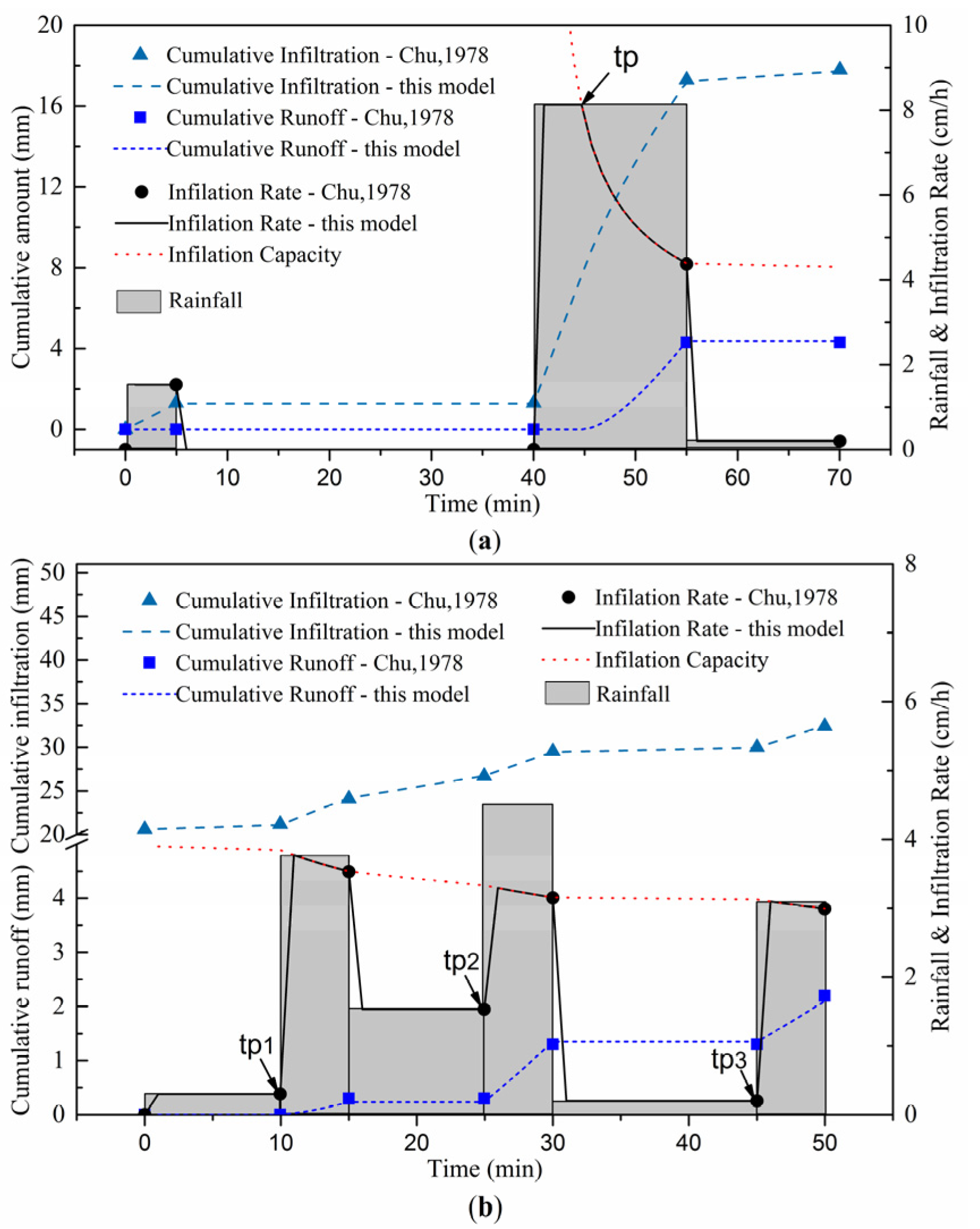
3.1. Homogeneous Soil during Unsteady Rainfall

The surface storage capacity S_c was 0, effective saturated hydraulic conductivity K_s was 1.42 cm/h, and the product of the effective suction (S) of the wetting front and the initial soil water deficit (M) was 3.6 cm. When the rainfall intensity was larger than the infiltration capacity, the infiltration-excess runoff occurred. The shift time was called the ponding moment. Only one ponding moment occurred in the first case and three ponding moments occurred in the second case. The infiltration-excess runoff ceased as rainfall intensity was smaller than the infiltration capacity. The rainfall intensity and decreasing infiltration capacity jointly controlled surface runoff generation. The calculated ponding time, infiltration volume, and infiltration rate of this proposed model were all consistent with Chu’s results (Figure 5).

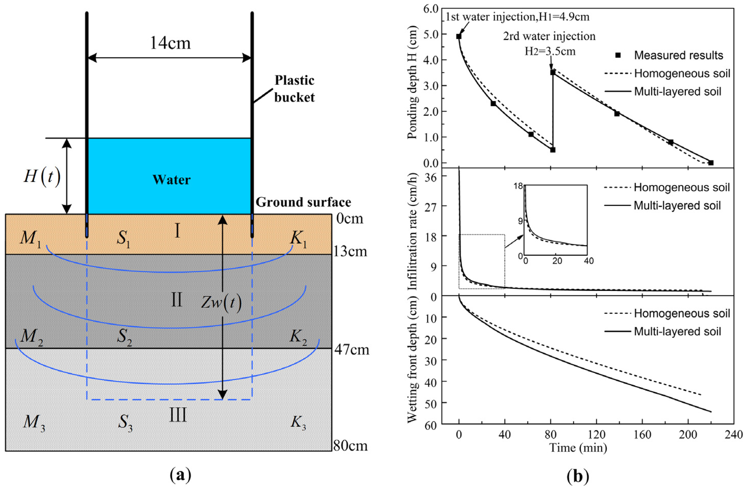
3.2. Ponding Infiltration Experiment on the Field

After the loose surface soil was cleaned, a plastic bucket of 14 cm-diameter was inserted into the soil surface. The height of the lower edge in the soil was about 1.5 cm (Figure 6a). Then, the Brilliant Blue solution was added into the bucket twice, 4.9 cm-depth for the first time (T = 0 min) and 3 cm-depth for the second time (T = 82 min). The falling ponding water depths in the bucket were recorded with a plastic ruler during the experiment.

Firstly, we assumed the soil column was homogeneous. The height of the simulated soil column was set as 60 cm. Each solution injection was simulated as a heavy rainfall with very short duration (10 s). The effective suction S of the wetting front was set as 20 cm based on soil textural classification [54,55]. Initial soil water deficit M was set as 0.17 according to the measured soil moisture data. The initial trial value of K_s was set as the average value of K_s (0.07 cm/min) in 0–10 cm. However, the simulated ponding depths were clearly overestimated. Then we increased the value of K_s by 15 percent of the last trial value. The final effective saturated hydraulic conductivity K_s was 0.018 cm/min. (

Table 2. Parameters of the ponding infiltration experiment case.

Homogeneous Case				Multilayered Case
Depth (cm)	$\mathit{M}$ (-)	S (cm)	Ks (cm/min)	Depth (cm)	$\mathit{M}$ (-)	S (cm)	Ks (cm/min)
0–60	0.17	20	0.018	0–13	0.17	20	0.022
				13–47	0.14	20	0.015
				47–60	0.12	20	0.012

).

The simulated ponding water depths after the first injection were larger than the measured values because of the underestimated infiltration rates (Figure 6b), whereas the simulated infiltration rates were slightly overestimated after the second injection. The RMSE and NSE of the homogeneous case were 0.166 cm and 0.988, respectively. Although the setting of homogeneous soil could describe the infiltration process generally, the accuracy needed to be improved further.

From field investigation, the surface soil was much looser and drier than the deeper soil. Therefore, the initial soil water deficit and effective saturated hydraulic conductivity should decrease with depth. Based on the soil genetic horizon, the 60 cm-height soil column was divided into three layers, i.e., 0–13 cm, 13–47 cm, and 47–60 cm. The calibrated parameters were referred to the homogeneous case. Specifically, the effective suction S of each layer was still set as 20 cm. Initial soil water deficit M of each layer was calculated based on the measured soil moisture data. We calibrated K_s from top to bottom and the initial trial value of each layer was set as 0.018 cm/min. The final calibrated parameters are shown in Table 2. The simulated ponding water depths in the multilayered case were better than that of the homogeneous case. The RMSE and NSE of the multilayered case was 0.035 cm and 0.999, respectively. By increasing the effective saturated hydraulic conductivity of the topsoil, the simulated infiltration rate after the first injection in the multilayered case became larger than that of the homogeneous case. Furthermore, when the wetting front advanced to deeper soil, the multilayered settings of initial soil water deficit and effective saturated hydraulic conductivity reduced the infiltration rate, which was more reasonable. The homogeneous case would underestimate the final wetting front depth in this experiment.

3.3. Rainfall–Runoff Events Simulation

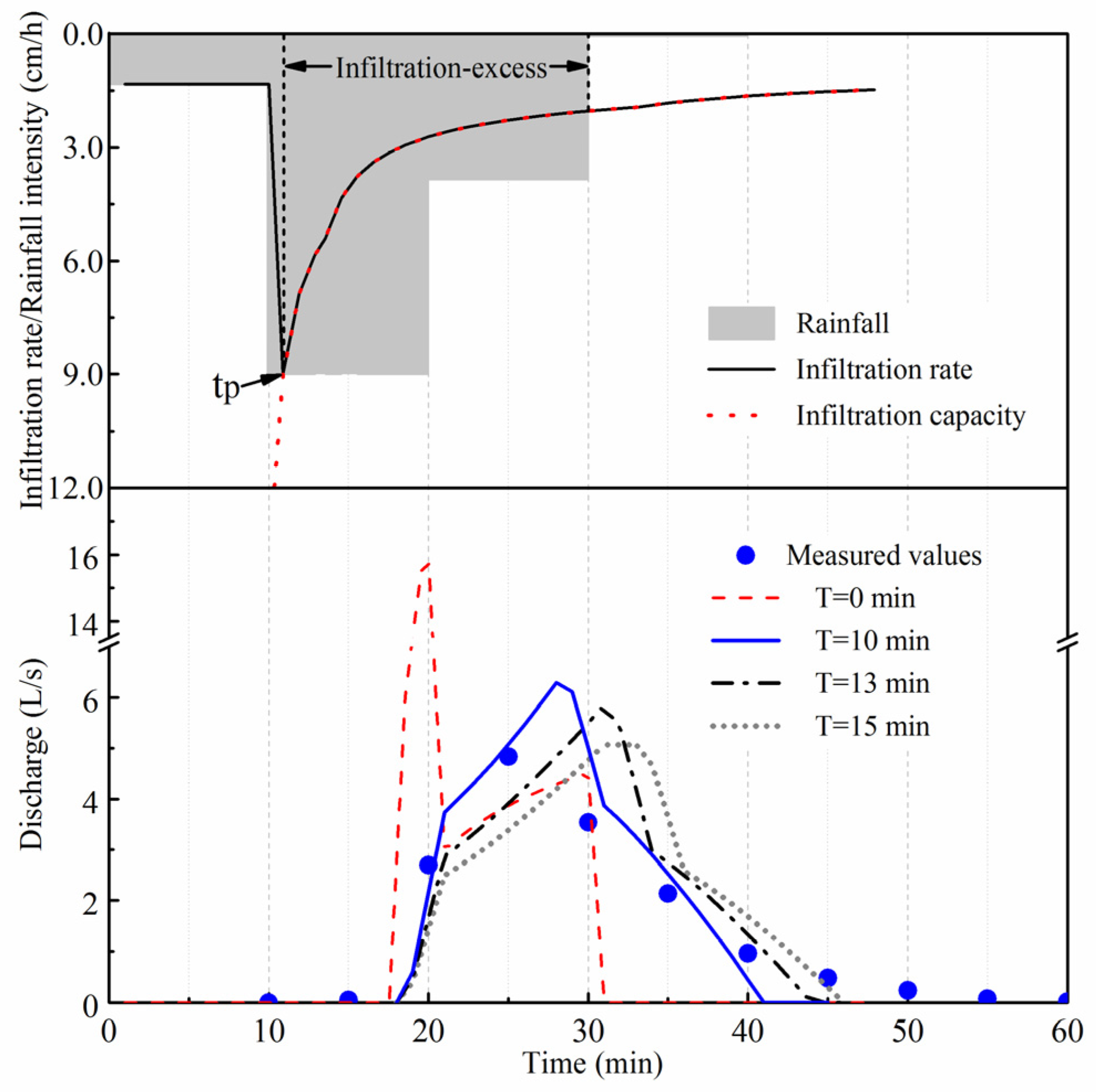
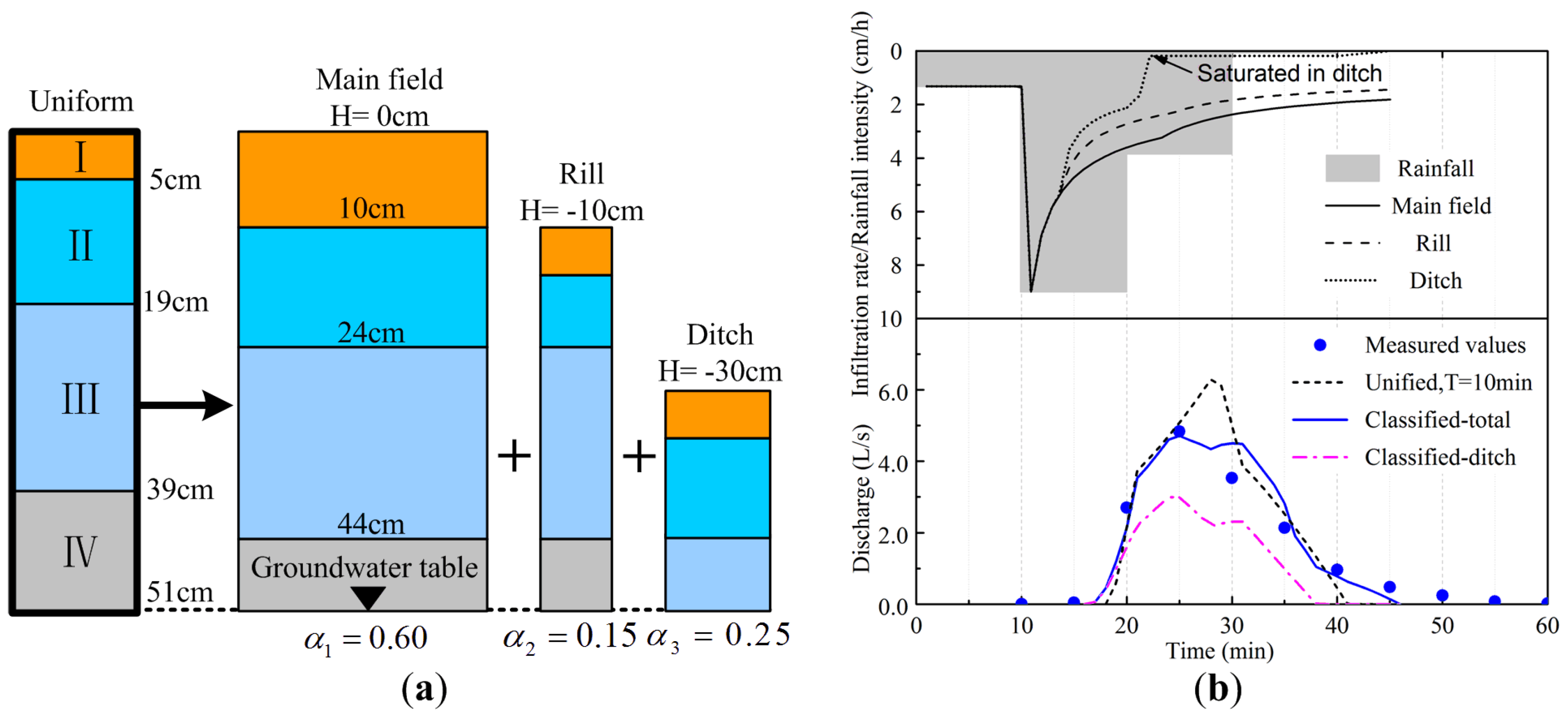
3.3.1. Typical Short-Duration Rainstorm Event

In order to identify the range of parameters, we calculated the unified topography case firstly.

a. Unified topography case

The thickness of the unsaturated zone was set as 51 cm based on the initial groundwater depth. According to the measured soil moisture data at various depths and the parameters derived from the previous infiltration experiment on the field, the unsaturated zone was divided into 4 layers (

Table 3. Parameters of 20160808 runoff case using the multilayered G–A model.

Layer Number	Depth (cm)	M (-)	S (cm)	Ks (cm/min)
I	0–5	0.130	20	0.018
II	5–19	0.062	20	0.015
III	19–39	0.028	20	0.015
IV	39–51	0.006	20	0.008

). The total soil water deficit was 21.5 mm, surface depression storage capacity S_c was 5 mm, Q_g was 0.01 mm/min. Average concentration time T was set as four levels, i.e., 0(direct outflow), 10, 13, and 15 min. The time step was set as one minute.

The rainfall intensity exceeded the surface infiltration capacity at the beginning of the second 10 min and ponding water started to appear on the surface (Figure 7). The final wetting front depth was 33.5 cm, not yet reaching the groundwater table, which means the soil water storage of the whole area was not saturated in the whole runoff process. Therefore, infiltration-excess mechanism was dominant. The simulated hydrograph of direct outflow (T = 0 min) was poor while the results of the other three cases were much better. Specifically, the case of 10 min fitted best. Therefore, the average concentration time in this rainfall event was approximately 10 min. The simulated runoff of 10 min case was 4.45 mm, close to the measured value. The RMSE and NSE was 0.43 L/s and 0.910, respectively. However, even in the case of 10 min, the simulated peak flow was still overestimated and the peak time lagged.

b. Classified topography case

Based on the previous unified topography case, parameters of three kinds of topographic subunits were calibrated. Due to the initial shallow groundwater, we moved the bottom of each layer of the main field 5 cm down so that the average soil water deficit of this case could be close to the unified case. Then, the bottom of each layer of rill and ditch referred to that of main field (

Table 4. Parameters of three kinds of topographic subunits in 20160808 runoff case.

Parameters	Main Field	Rill	Ditch
$\alpha$ (/)	0.6	0.15	0.25
$\overline{H}$ (cm)	0	−10	−30
$S_c$ (mm)	5	4	3.5
T(min)	14	10	7
Layer(cm)	I (0–10)	I (0–5)	I (0–5)
	II (10–24)	II (5–14)	II (5–14)
	III (24–44)	III (14–34)	III (14–21)
	IV (44–51)	IV (34–41)	-

, Figure 8a). A soil layer number corresponded to a specific set of Green–Ampt parameters. The concentration time of the ditch was the shortest while that of the main field was the longest. The concentration time of the rill was set as the average value, which was applied in the unified topography case. The average elevations of three topographic subunits were based on topographic statistics, in which the relative elevation of the main field was set as 0 cm. The time step was the same as in the unified topography case.

The simulated hydrograph of classified topography case fitted better compared with the unified topography case (T = 10 min). The simulated runoff of this case was 4.86 mm, slightly larger than the measured value. The RMSE and NSE was 0.33L/s and 0.94, respectively. The discharge in 30–35 min was slightly overestimated (Figure 8b). The ponding time of each subunit was almost the same. Notably, soil water storage of the ditch had been saturated since the 22nd min, which was different from the results of the unified case. Therefore, infiltration-excess mechanism under saturated condition was dominant in the ditch since then. The peak discharge of the ditch was 3.0 L, accounting for 65% of the corresponding total discharge. The simulated shallow groundwater discharge of the ditch was about 0.19 mm.

The water balance items of three topographic subunits are shown in

Table 5. Parameters of three kinds of topographic subunits in 20160808 runoff case.

Parameter	Main Field	Rill	Ditch
WFD/UZT (cm)	23/51	36/41	21/21
Subunit infiltration (mm)	21.1	18.1	13.8
Subunit runoff (mm)	2.6	5.6	9.9
Area ratio (-)	0.60	0.15	0.25
Converted total runoff(mm)	1.54	0.84	2.48
Runoff ratio (-)	0.32	0.17	0.51
Runoff ratio/Area ratio (-)	0.5	1.1	2.0

. The higher the surface elevation was, the greater the infiltration was, while the smaller the runoff was. The runoff of the ditch accounted for 51% of the total runoff, about twice of its area ratio. The runoff contribution of main field was 0.32, only half of its area ratio. The runoff contribution of rill was slightly larger than its area ratio. Therefore, massive surface runoff was generated from the low-lying ditch during the infiltration-excess period under saturated condition in this case, resulting in an advance in peak time and reduction in flood peak.

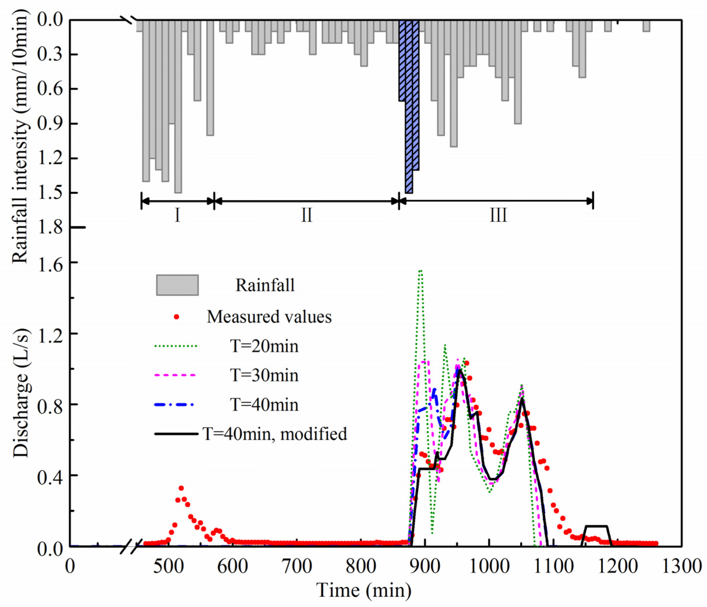
3.3.2. Typical Long-Duration Light Rainfall Event

We calculated the unified topography case firstly to identify the parameters.

a. Unified topography case

The thickness of the unsaturated zone was set as 95 cm. Combining the infiltration experiment case and measured multilayered soil moisture data, the unsaturated zone was divided into 5 layers (

Table 6. Parameters of Layered G–A model for 20160406 rainfall–runoff event.

Layer Number	Depth (cm)	M (-)	S (cm)	Ks (cm/min)
I	0–5	0.094	20	0.018
II	5–19	0.029	20	0.015
III	19–34	0.035	20	0.015
IV	34–60	0.024	20	0.008
V	60–95	0.013	20	0.005

). S_c was 5 mm and Q_g was 0.01 mm/min. The concentration time was set as 20, 30, and 40 min. Time step was set as one minute.

The case of 40 min showed the best-fitting results (Figure 9). Therefore, the average concentration time could be close to 40 min. In contrast, this average concentration time was four times the value of the previous short-duration rainstorm runoff case. It was inferred that the runoff caused by light rainfall spent a much longer time reaching the outlet than that caused by intense rainfall. The simulated runoff was 8.8 mm, less than the measured value. Remarkably, the first stage of outflow occurring in period I (500–600th min), in which the discharge was small, could not be simulated. It is obvious that topography homogenization setting could not grasp such a relatively small outflow process in the early stage. Furthermore, the simulated discharges of three cases in the early phase of period III were all overestimated. Notably, the rain intensity was smaller than the smallest saturated hydraulic conductivity (0.005 cm/min) during period II (lasting about 4 h). Therefore, the ponding water in surface storage should recede gradually in this period, resulting in a newly arising surface storage deficit. However, such process could not be represented in this proposed model. We improved groundwater discharge rate to 0.05 mm/min in the early phase of period III (860–900th min) temporarily in the case of 40 min to fill the newly arising surface storage deficit. The hydrograph of 40 min after modifying was much better in the early phase of period III. The NSE and RMSE of the simulated hydrograph of 40 min after modifying between the 485th and 1205th min were 0.817 and 0.11 L/s, respectively.

b. Classified topography case

The parameters of different soil layers and calibrated concentration time of three kinds of topographic subunits are shown in

Table 7. Model parameters of three kinds of topographic subunits in 20160406 rainfall event.

Parameter	Main Field	Rill	Ditch
T(min)	40	35	25
Layers(cm)	I (0–5)	I (0–5)	I (0–5)
	II (5–19)	II (5–9)	II (5–10)
	III (19–34)	III (9–24)	III (10–20)
	IV (34–60)	IV (24–50)	IV (20–30)
	V (60–95)	V (50–85)	V (30–65)

and Figure 10a. The groundwater discharge rates were 0.01 mm/min. The discharge rate for the rill and ditch were 0.06 mm/min between the 860th and 900th min, and 0.04 mm/min for the main field. The surface storage and other parameters were the same as the typical short-duration rainstorm case.

The outflow of three kinds of topographic subunits occurred at different moments (Figure 10b). The lower the average elevation was, the earlier the outflow occurred. The ditch outflowed first at the 484th min, the rill outflowed at the 544th min, and the main field outflowed last at the 878th min. Clearly, only the ditch and rill were involved in the initial outflow process (period I) and we called that period partial outflow. The partial outflow process could be grasped after classifying topography and the whole simulated hydrograph fitted quite well with the measured one. The simulated runoff increased to 9.6 mm. The NSE between 485th and 1205th min increased to 0.916 and the RMSE decreased to 0.08 L/s.

Although the main field was the last to outflow, it contributed half of the total runoff (

Table 8. Statistics of three kinds of topographic subunits in 20160406 runoff case.

Parameter	Main Field	Rill	Ditch
WFD/UZT (cm)	95/95	85/85	65/65
Subunit infiltration (mm)	40.0	36.8	35.1
Subunit Runoff (mm)	7.9	11.1	12.8
Area ratio (-)	0.6	0.15	0.25
Converted total runoff (mm)	4.7	1.7	3.2
Runoff ratio (-)	0.49	0.18	0.33
Runoff ratio/Area ratio (-)	0.8	1.2	1.3

). The runoff rate of each subunit was basically the same as the area ratio. Therefore, microtopography had a clear impact on initial partial outflow process while it had little effect on runoff when the whole area was saturated. The topography classification method could greatly improve simulation accuracy of the initial partial outflow process occurring in the low-lying areas.

4. Discussion

In the typical short-duration rainstorm event (20160808), the ditch played a dominant role. The runoff of the ditch accounted for 51% of the total runoff, about twice of its area ratio. The runoff contribution of main field was 0.32, only half of its area ratio. It is because the infiltration-excess regime under saturated condition was dominant in the ditch and the runoff coefficient was extremely high during that period. However, neither the main field nor rill were saturated during the rainfall; they were dominated by infiltration-excess regime accompanied with considerable infiltration, which restricted the runoff coefficients of these two topographic subunits. Ditch networks indeed accelerate runoff by concentrating the flow and avoiding natural obstacles [28],which reduces the peak flow discharge [56].

In the typical long-duration light rainfall event (20160406), the ditch and rill became saturated successively and played a dominant role in the first runoff. Although the first runoff was small (0.8 mm), it was an important period for nutrient exporting [57]. When the highest main field was saturated, the whole area was dominated by saturation excess regime and the main field with the largest area contributed the most runoff. Therefore, microtopography had a clear impact on initial partial outflow process while it had little effect on runoff when the whole area was saturated, which agreed with Chen’s conclusion [22].

We adopted the average concentration time method to simplify the concentration process. The results of two typical rainfall events show that the method was effective and applicable for plot scale without significant topographic slope. The average concentration time was affected by both rainfall intensity and microtopography. The greater the rainfall intensity, the shorter the average concentration time. The lower topographic subunit is normally the man-made drainage channels corresponding to shorter concentration pathway and shorter average concentration time.

Nevertheless, this proposed model cannot represent the receding surface ponding water process during a long period of very light rainfall when soil water storage has been saturated. Therefore, the layered G–A model considering redistribution of soil water during intermittent rainfall needs to be expanded in later studies [58,59,60]. Additionally, the lateral subsurface flow between each of the two topographic subunits was ignored in this proposed model. However, the groundwater of low topographic subunit usually responds rapidly to intense rainfall, which may cause regional groundwater head gradient and lateral subsurface flow. Such phenomenon would influence temporal soil water shortage and runoff of relatively high units. It is necessary to consider the influence of subsurface flow in the future.

Furthermore, sensitivity and uncertainty analysis [61] as well as an automatic calibration module [62] are needed to acquire the parameters of three topographic subunits more effectively and accurately.

5. Conclusions

An event-based rainfall–runoff model considering microtopographic features of plot scale in plain farmland areas was proposed in this paper. Various experimental scenarios were simulated, including two classical unsteady rainfall events in homogeneous soil, one ponding infiltration experiment, and two typical rainfall–runoff events (i.e., short-duration rainstorm and long-duration light rainfall) in the experimental field. The findings can be summarized as follows:

(1) The multilayered setting showed higher accuracy than the homogeneous setting for simulating infiltration. The RMSE of simulated ponding water depth in the ponding infiltration experiment reduced from 0.166 cm to 0.035 cm and NSE rose from 0.988 to 0.999. The accuracy of simulated hydrograph using the proposed model considering microtopography effects proved higher than that under unified topography assumption.

(2) The lower the topographic subunit, the earlier the outflow occurred. The runoff mostly originated from the relatively low topographic subunits (i.e., ditch and rill) at the early stage. Infiltration-excess regime under saturated condition may initially dominate in the low-lying ditch under intense rainfall, with extremely high runoff coefficient.

(3) The concentration process in the plain farmland area was affected by both rainfall intensity and microtopography. The intense rainfall corresponded to short average concentration time. The average concentration velocity under heavy rainfall was four times faster than that under light rainfall. The lower topographic subunit was characterized by shorter average concentration time. Ditches reduced the peak flow and advanced the time to peak.

References

1. Yan, R.; Li, L.; Gao, J. Framework for quantifying rural NPS pollution of a humid lowland catchment in Taihu Basin, Eastern China. Sci. Total Environ. 2019, 688, 983–993. [Google Scholar] [CrossRef] [PubMed]
2. Appels, W.M.; Bogaart, P.W.; van der Zee, S.E.A.T.M. Feedbacks Between Shallow Groundwater Dynamics and Surface Topography on Runoff Generation in Flat Fields. Water Resour. Res. 2017, 53, 10336–10353. [Google Scholar] [CrossRef]
3. Van der Ploeg, M.J.; Appels, W.M.; Cirkel, D.G.; Oosterwoud, M.R.; Witte, J.-P.M.; van der Zee, S.E.A.T.M. Microtopography as a Driving Mechanism for Ecohydrological Processes in Shallow Groundwater Systems. Vadose Zone J. 2012, 11, 811–822. [Google Scholar] [CrossRef]
4. Thompson, S.E.; Katul, G.G.; Porporato, A. Role of microtopography in rainfall-runoff partitioning: An analysis using idealized geometry. Water Resour. Res. 2010, 46, 58–72. [Google Scholar] [CrossRef]
5. Frei, S.; Fleckenstein, J.H. Representing effects of micro-topography on runoff generation and sub-surface flow patterns by using superficial rill/depression storage height variations. Environ.Model. Softw. 2014, 52, 5–18. [Google Scholar] [CrossRef]
6. Chu, X.; Nelis, J.; Rediske, R. Preliminary Study on the Effects of Surface Microtopography on Tracer Transport in a Coupled Overland and Unsaturated Flow System. J. Hydrol. Eng. 2013, 18, 1241–1249. [Google Scholar] [CrossRef]
7. Appels, W.M.; Bogaart, P.W.; van der Zee, S.E.A.T.M. Influence of spatial variations of microtopography and infiltration on surface runoff and field scale hydrological connectivity. Adv. Water Resour. 2011, 34, 303–313. [Google Scholar] [CrossRef]
8. Chu, X.; Yang, J.; Chi, Y.; Zhang, J. Dynamic puddle delineation and modeling of puddle-to-puddle filling-spilling-merging-splitting overland flow processes. Water Resour. Res. 2013, 49, 3825–3829. [Google Scholar] [CrossRef]
9. Tayfur, G.; Kavvas, M. Spatially Averaged Conservation Equations for Interacting Rill-Interrill Area Overland Flows. J. Hydraul. Eng. 1994, 120, 1426–1448. [Google Scholar] [CrossRef]
10. Tayfur, G.; Kavvas, M.L. Areally-averagei overland flow equations at hillslope scale. Hydrol. Sci. J. 1998, 43, 361–378. [Google Scholar] [CrossRef] [Green Version]
11. Herzon, I.; Helenius, J. Agricultural drainage ditches, their biological importance and functioning. Biol. Conserv. 2008, 141, 1171–1183. [Google Scholar] [CrossRef]
12. Buchanan, B.; Easton, Z.M.; Schneider, R.L.; Walter, M.T. Modeling the hydrologic effects of roadside ditch networks on receiving waters. J. Hydrol. 2013, 486, 293–305. [Google Scholar] [CrossRef]
13. Planchon, O.; Esteves, M.; Silvera, N.; Lapetite, J.-M. Microrelief induced by tillage: Measurement and modelling of Surface Storage Capacity. Catena 2001, 46, 141–157. [Google Scholar] [CrossRef]
14. Khosh Bin Ghomash, S.; Caviedes-Voullieme, D.; Hinz, C. Effects of erosion-induced changes to topography on runoff dynamics. J. Hydrol. 2019, 573, 811–828. [Google Scholar] [CrossRef]
15. Habtezion, N.; Nasab, M.T.; Chu, X. How Does DEM Resolution Affect Microtopographic Characteristics, Hydrologic Connectivity, and Modeling of Hydrologic Processes? Hydrol. Processes 2016, 30, 4870–4892. [Google Scholar] [CrossRef]
16. Carvajal, F.; Aguilar, M.A.; Agüera, F.; Aguilar, F.J.; Giráldez, J.V. Maximum Depression Storage and Surface Drainage Network in Uneven Agricultural Landforms. Biosyst. Eng. 2006, 95, 281–293. [Google Scholar] [CrossRef]
17. Hansen, B. Estimation of surface runoff and water-covered area during filling of surface microrelief depressions. Hydrol. Processes 2000, 14, 1235–1243. [Google Scholar] [CrossRef]
18. Frei, S.; Lischeid, G.; Fleckenstein, J.H. Effects of micro-topography on surface–subsurface exchange and runoff generation in a virtual riparian wetland—A modeling study. Adv. Water Resour. 2010, 33, 1388–1401. [Google Scholar] [CrossRef]
19. Dunne, T.; Zhang, W.; Aubry, B.F. Effects of Rainfall, Vegetation, and Microtopography on Infiltration and Runoff. Water Resour. Res. 1991, 27, 2271–2285. [Google Scholar] [CrossRef]
20. Chu, X.; Padmanabhan, G.; Bogart, D. Microrelief-Controlled Overland Flow Generation: Laboratory and Field Experiments. Appl. Environ. Soil Sci. 2015, 2015, 642952. [Google Scholar] [CrossRef] [Green Version]
21. Appels, W.M.; Bogaart, P.W.; van der Zee, S.E.A.T.M. Surface runoff in flat terrain: How field topography and runoff generating processes control hydrological connectivity. J. Hydrol. 2016, 534, 493–504. [Google Scholar] [CrossRef]
22. Chen, L.; Sela, S.; Svoray, T.; Assouline, S. The role of soil-surface sealing, microtopography, and vegetation patches in rainfall-runoff processes in semiarid areas. Water Resour. Res. 2013, 49, 5585–5599. [Google Scholar] [CrossRef]
23. Frei, S.; Knorr, K.H.; Peiffer, S.; Fleckenstein, J.H. Surface micro-topography causes hot spots of biogeochemical activity in wetland systems: A virtual modeling experiment. J. Geophys. Res. Biogeosci. 2012, 117, G4. [Google Scholar] [CrossRef]
24. Antoine, M.; Javaux, M.; Bielders, C. What indicators can capture runoff-relevant connectivity properties of the micro-topography at the plot scale? Adv. Water Resour. 2009, 32, 1297–1310. [Google Scholar] [CrossRef]
25. Yang, J.; Chu, X. Quantification of the spatio-temporal variations in hydrologic connectivity of small-scale topographic surfaces under various rainfall conditions. J. Hydrol. 2013, 505, 65–77. [Google Scholar] [CrossRef]
26. Aksoy, H.; Gedikli, A.; Unal, N.E.; Yilmaz, M.; Eris, E.; Yoon, J.; Tayfur, G. Rainfall-Runoff Model Considering Microtopography Simulated in a Laboratory Erosion Flume. Water Resour. Manag. 2016, 30, 5609–5624. [Google Scholar] [CrossRef]
27. Mallari, K.J.B.; Arguelles, A.C.C.; Kim, H.; Aksoy, H.; Kavvas, M.L.; Yoon, J. Comparative analysis of two infiltration models for application in a physically based overland flow model. Environ. Earth Sci. 2015, 74, 1579–1587. [Google Scholar] [CrossRef]
28. Moussa, R.; Voltz, M.; Andrieux, P. Effects of the spatial organization of agricultural management on the hydrological behaviour of a farmed catchment during flood events. Hydrol. Processes 2002, 16, 393–412. [Google Scholar] [CrossRef]
29. Carluer, N.; Marsily, G.D. Assessment and modelling of the influence of man-made networks on the hydrology of a small watershed: Implications for fast flow components, water quality and landscape management. J. Hydrol. 2004, 285, 76–95. [Google Scholar] [CrossRef]
30. Tiemeyer, B.; Moussa, R.; Lennartz, B.; Voltz, M. MHYDAS-DRAIN: A spatially distributed model for small, artificially drained lowland catchments. Ecol. Model. 2007, 209, 2–20. [Google Scholar] [CrossRef]
31. Haahti, K.; Warsta, L.; Kokkonen, T.; Younis, B.A.; Koivusalo, H. Distributed hydrological modeling with channel network flow of a forestry drained peatland site. Water Resour. Res. 2016, 52, 246–263. [Google Scholar] [CrossRef]
32. VanderKwaak, J.E.; Loague, K. Hydrologic-Response simulations for the R-5 catchment with a comprehensive physics-based model. Water Resour. Res. 2001, 37, 999–1013. [Google Scholar] [CrossRef]
33. Jain, A.; Indurthy, S.K.V.P. Comparative Analysis of Event-based Rainfall-runoff Modeling Techniques—Deterministic, Statistical, and Artificial Neural Networks. J. Hydrol. Eng. 2003, 8, 93–98. [Google Scholar] [CrossRef]
34. Tramblay, Y.; Bouvier, C.; Martin, C.; Didon-Lescot, J.-F.; Todorovik, D.; Domergue, J.-M. Assessment of initial soil moisture conditions for event-based rainfall–runoff modelling. J. Hydrol. 2010, 387, 176–187. [Google Scholar] [CrossRef]
35. Escobar-Ruiz, V.; Smith, H.G.; Macdonald, N.; Peñuela, A. Simulated event-scale flow and sediment generation responses to agricultural land cover change in lowland UK catchments. Hydrol. Processes 2022, 36, e14474. [Google Scholar] [CrossRef]
36. Tian, P.; Feng, J.; Zhao, G.; Gao, P.; Sun, W.; Hörmann, G.; Mu, X. Rainfall, runoff, and suspended sediment dynamics at the flood event scale in a Loess Plateau watershed, China. Hydrol. Processes 2022, 36, e14486. [Google Scholar] [CrossRef]
37. Wang, H.; Wang, H.; Li, H.; Faisal, M.; Zhang, Y. Analysis of drainage efficiency under extreme precipitation events based on numerical simulation. Hydrol. Processes 2022, 36, e14624. [Google Scholar] [CrossRef]
38. Cerdan, O.; Le Bissonnais, Y.; Govers, G.; Lecomte, V.; van Oost, K.; Couturier, A.; King, C.; Dubreuil, N. Scale effect on runoff from experimental plots to catchments in agricultural areas in Normandy. J. Hydrol. 2004, 299, 4–14. [Google Scholar] [CrossRef]
39. Hua, W.; Wang, C.; Chen, G.; Yang, H.; Zhai, Y. Measurement and Simulation of Soil Water Contents in an Experimental Field in Delta Plain. Water 2017, 9, 947. [Google Scholar] [CrossRef]
40. Zhai, Y.; Wang, C.; Chen, G.; Wang, C.; Li, X.; Liu, Y. Field-Based Analysis of Runoff Generation Processes in Humid Lowlands of the Taihu Basin, China. Water 2020, 12, 1216. [Google Scholar] [CrossRef]
41. Green, W.H.; Ampt, G.A. Studies on Soil Phyics. J. Agric. Sci. 1911, 4, 1–24. [Google Scholar] [CrossRef]
42. Kale, R.V.; Sahoo, B. Green-Ampt Infiltration Models for Varied Field Conditions: A Revisit. Water Resour. Manag. 2011, 25, 3505–3536. [Google Scholar] [CrossRef]
43. Sander, T.; Gerke, H.H. Preferential Flow Patterns in Paddy Fields Using a Dye Tracer. Vadose Zone J. 2007, 6, 105–115. [Google Scholar] [CrossRef]
44. Mishra, S.K.; Sarkar, R.; Dutta, S.; Panigrahy, S. A physically based hydrological model for paddy agriculture dominated hilly watersheds in tropical region. J. Hydrol. 2008, 357, 389–404. [Google Scholar] [CrossRef]
45. Tan, X.; Shao, D.; Gu, W.; Liu, H. Field analysis of water and nitrogen fate in lowland paddy fields under different water managements using HYDRUS-1D. Agric. Water Manag. 2015, 150, 67–80. [Google Scholar] [CrossRef]
46. Tan, X.; Shao, D.; Liu, H. Simulating soil water regime in lowland paddy fields under different water managements using HYDRUS-1D. Agric. Water Manag. 2014, 132, 69–789. [Google Scholar] [CrossRef]
47. Liu, J.; Zhang, J.; Feng, J. Green–Ampt Model for Layered Soils with Nonuniform Initial Water Content Under Unsteady Infiltration. Soil Sci. Soc. Am. J. 2008, 72, 1041–1047. [Google Scholar] [CrossRef]
48. Kroes, J.G.; Dam, J.C.v.; Bartholomeus, R.P.; Groenendijk, P.; Heinen, M.; Hendriks, R.F.A.; Mulder, H.M.; Supit, I.; van Walsum, P.E.V. SWAP Version 4, Theory Description and User Manual; 1566-7197; Wageningen Environmental Research: Wageningen, The Netherlands, 2017; p. 244. [Google Scholar]
49. Beven, K.J. A history of the concept of time of concentration. Hydrol. Earth Syst. Sci. 2020, 24, 2655–2670. [Google Scholar] [CrossRef]
50. Zhao, L.; Wu, F. Simulation of Runoff Hydrograph on Soil Surfaces with Different Microtopography Using a Travel Time Method at the Plot Scale. PLoS ONE 2015, 10, e0130794. [Google Scholar]
51. Du, J.; Xie, H.; Hu, Y.; Xu, Y.; Xu, C.-Y. Development and testing of a new storm runoff routing approach based on time variant spatially distributed travel time method. J. Hydrol. 2009, 369, 44–54. [Google Scholar] [CrossRef]
52. Nash, J.E.; Sutcliffe, J.V. RiverRiver flow forecasting through conceptual models part I—A discussion of principles. J. Hydrol. 1970, 10, 282–290. [Google Scholar] [CrossRef]
53. Chu, S.T. Infiltration during an unsteady rain. Water Resour. Res. 1978, 14, 461–466. [Google Scholar] [CrossRef]
54. Rawls, W.J.; Brakensiek, D.L. Estimating Soil Water Retention from Soil Properties. J. Irrig. Drain. Div. 1982, 108, 166–171. [Google Scholar] [CrossRef]
55. Rawls, W.J.; Brakensiek, D.L.; Miller, N. Green-ampt Infiltration Parameters from Soils Data. J. Hydraul. Eng. 1983, 109, 62–70. [Google Scholar] [CrossRef]
56. Barber, M.E.; King, S.G.; Yonge, D.R.; Hathhorn, W.E. Ecology Ditch: A Best Management Practice for Storm Water Runoff Mitigation. J. Hydrol. Eng. 2003, 8, 111–122. [Google Scholar] [CrossRef]
57. Li, S.; Wang, X.; Qiao, B.; Li, J.; Tu, J. First flush characteristics of rainfall runoff from a paddy field in the Taihu Lake watershed, China. Environ. Sci. Pollut. Res. 2017, 24, 8336–8351. [Google Scholar] [CrossRef]
58. Muñoz-Carpena, R.; Lauvernet, C.; Carluer, N. Shallow water table effects on water, sediment, and pesticide transport in vegetative filter strips—Part 1: Nonuniform infiltration and soil water redistribution. Hydrol. Earth Syst. Sci. 2018, 22, 53–70. [Google Scholar] [CrossRef]
59. Gowdish, L.C.; Muñoz-Carpena, R. 3DMGAR: A Transient Quasi-3D Point-Source Green–Ampt Infiltration and Redistribution Model. Vadose Zone J. 2018, 17, 180032. [Google Scholar] [CrossRef]
60. Gowdish, L.; Muñoz-Carpena, R. An Improved Green–Ampt Infiltration and Redistribution Method for Uneven Multistorm Series. Vadose Zone J. 2009, 8, 470–479. [Google Scholar] [CrossRef]
61. Fernández-Pato, J.; Caviedes-Voullième, D.; García-Navarro, P. Rainfall/runoff simulation with 2D full shallow water equations: Sensitivity analysis and calibration of infiltration parameters. J. Hydrol. 2016, 536, 496–513. [Google Scholar] [CrossRef]
62. Doherty, J. PEST model-independent parameter estimation user manual. Watermark Numer. Comput. Brisb. Aust. 2004, 3338, 3349. [Google Scholar]
Figure 1. Information of the experimental field: (a) location of Hongqi polder; (b) land use of Hongqi polder; (c) location of the experimental field.
Water 14 02686 g001
Figure 2. (a) Topography (0.1 m−resolution DEM) and layout of the experimental field; (b) three−dimensional view of the isolated catchment; (c) section shape of western ditch; (d) section shape of eastern ditch.
Water 14 02686 g002
Figure 3. Schematic representation of the Green–Ampt model for layered soils under nonsteady rainfall infiltration.
Water 14 02686 g003
Figure 4. Schematic of rainfall–runoff model considering effects of microtopography: (a) a rainfall–runoff event at the field; (b) model structure.
Water 14 02686 g004
Figure 5. Homogeneous soil during unsteady rainfalls: (a) 30 June 1957; (b) 3 April 1958.
Water 14 02686 g005
Figure 6. Ponding infiltration experiment on the field: (a)schematic diagram; (b) modeling results of homogeneous and multilayered cases.
Water 14 02686 g006
Figure 7. Simulated hydrographs of different concentration time in unified topography case in 20160808 rainfall event.
Water 14 02686 g007
Figure 8. The 20160808 runoff case considering the effect of microtopography: (a) classified topography setting; (b) observed and simulated results.
Water 14 02686 g008
Figure 9. Observed and simulated hydrographs of unified topography cases of different concentration times in 20160406 rainfall event.
Water 14 02686 g009
Figure 10. The 20160406 runoff case considering the effect of microtopography: (a) classified topography setting; (b) simulation results.
Water 14 02686 g010