
Copula-Based Multivariate Simulation Approach for Flood Risk Transfer of Multi-Reservoirs in the Weihe River, China
by
Shen Wang
1,
Jing Wu
1,
Siyi Wang
1,
Xuesong Xie
1,
Yurui Fan
2,
Lianhong Lv
1,* and
Guohe Huang
3 1
Chinese Research Academy of Environmental Sciences, Beijing 100012, China
2
College of Engineering, Design and Physical Sciences, Brunel University London, Uxbridge UB8 3PH, UK
3
State Key Joint Laboratory of Environmental Simulation and Pollution Control, CEEER-URBNU, College of Environment, Beijing Normal University, Beijing 100875, China
*
Author to whom correspondence should be addressed.
Water 2022, 14(17), 2676; https://doi.org/10.3390/w14172676
Submission received: 11 July 2022
/
Revised: 17 August 2022
/
Accepted: 26 August 2022
/
Published: 29 August 2022
(This article belongs to the Section Hydrology)
Abstract
:The interplay of multi-reservoirs is critical in reservoir joint disposal and water conservancy projects. As the flood risk of upstream hydrological stations could be transferred and unevenly distributed to downstream tributary stations, flood risk transfer through multi-reservoirs warrants further investigation. This study proposed a copula simulation approach to develop a joint flood risk distribution of multi-reservoirs (spanning Xianyang, Huaxian County, and Zhangjiashan) in a drainage tributary of the Weihe River. Pair-copulas of each reservoir pair were constructed to analyse the correlations between the reservoir sites. The approach was then used to create a joint flood risk distribution for the reservoirs. The flood risk and corresponding flood volume of Zhangjiashan were calculated based on the flood risk levels of Xianyang and Huaxian County. The results indicate that the flood risks of Huaxian County would be transferred to Xianyang and Zhangjiashan to some extent, and Xianyang could mitigate more flood risks from Huaxian County than from Zhangjiashan. The findings have significance for informed decision-making regarding the Zhangjiashan reservoir construction project.
1. Introduction
Floods are one of the most common natural hazards that frequently endanger both human life and the environment. Reservoirs are the most crucial infrastructure to ensure safety in a drainage tributary during floods. The simultaneous construction and disposal of reservoirs have essential significance for complex water conservancy projects. Flood risk also plays an essential role in the joint disposal and construction of reservoirs. Risk analysis of floods is one of the most critical requirements in reservoir design. According to drainage basin and sub-basin scales, flood risk is mainly attributable to rainfall and sub-basin relationships. It is difficult to forecast flash floods owing to their dynamic and complex nature [1,2,3,4,5]. In addition, comprehensive hydrological data can be challenging to obtain as these involve complex variables [6]. Moreover, the reservoirs of adjacent tributaries exhibit significant correlations [7,8,9]. Therefore, joint flood risk studies are a priority for reservoir construction and the disposal of adjacent tributaries.
Studies on joint flood risks for multi-reservoirs systems are challenging. Various approaches have been proposed and developed for flood risk and streamflow studies. Prairie et al. [10] introduced a stochastic nonparametric technique for the spatiotemporal disaggregation of streamflows. Hao and Singh [11] developed a modelling approach for multisite streamflow dependence based on the maximum entropy copula. Chen et al. [12] introduced a copula-based method for multisite monthly and daily streamflow simulations. The copula-based method provides a new tool for multisite stochastic simulations and flood risk studies.
Research on flood risk transfer in multi-reservoirs has been relatively sparse. In most traditional studies, multivariate problems of joint flood risks are mainly translated into bivariate cases. Krstanovic and Singh [13] used a bivariate distribution to obtain a joint distribution of flood peaks and volumes. They reported that a bivariate distribution could describe some features of floods. Yue [14] introduced a bivariate lognormal distribution to model a multivariate flood episode. Escalante-Sandoval [15] applied a bivariate extreme value distribution for flood frequency analysis in northwestern Mexico. Trivariate distributions have rarely been used for flood frequency and risk analysis. Sandoval and Raynal-Villaseñor [16] used a trivariate generalised extreme value distribution for flood frequency analysis. Therefore, an effective method of high-dimensional joint distribution has unique advantages in risk studies for the flood risk transfer of multi-reservoirs.
The copula method is one of the most effective methods for determining joint distributions. High-dimensional copula functions have been applied to hydrological datasets to perform rainfall frequency and flood frequency analyses, respectively [17,18]. Recently, copulas have been applied to stochastic simulations of hydrological data. Copulas have many advantages in hydrology, such as flexibility in the choice of arbitrary marginal distributions, extending to multivariables and permitting separate analysis of marginal distributions and dependence structure. Pinya et al. [19] applied a copula model to assess flooding risks in a tidal sluice-regulated catchment. Copulas are flexible joint distributions that can handle mixed marginal distributions [20,21,22,23]. Bárdossy and Pegram [24] used the copula method for multisite daily precipitation simulations. The copula function can describe the dependence between random input variables and apply these to arbitrary marginal distribution types of random variables with no linear dependence constraints. Therefore, it is an effective tool for joint flood risk studies.
The objective of this study was to implement the copula method to construct a multisite joint flood risk distribution in a drainage tributary of the Weihe River. The Weihe River is the largest tributary of the Wei River, which, in turn, is the largest tributary of the Yellow River. This drainage tributary includes three reservoir sites: Xianyang, Huaxian County, and Zhangjiashan. While reservoirs have already been constructed at Xianyang and Huaxian County, the results of this study can provide constructive suggestions for the Zhangjiashan reservoir construction project. Generated flow data can serve as useful input for reservoir design, risk assessment, and the reliability of water resource systems. Moreover, the flood risk distribution of multi-reservoirs using a copula-based approach can provide new insights into reservoir joint disposal and reservoir risk control.
2. Materials and Methods
This section outlines the proposed copula method for constructing a joint flood risk distribution of multi-reservoirs. This method aims to generate the flood risk level of the primary reservoir, based on flood risk levels near other reservoir sites. Several hypotheses were considered in this study. The marginal distributions are Pearson type 3. Copula families do not cover all behaviours, especially for extreme dependencies. Extreme dependencies are non-existent between each pair of the hydrometric station. The behaviours of all pairs of hydrometric stations are not complicated in this study. Therefore, copulas were deemed suitable for this study.
2.1. Copula Method
A copula is a joint distribution function of standard uniform random variables. It can be represented as:
It must fulfil the following conditions:
where, and are the marginal distributions.
Subsequently, the n dimensional distribution function F can be written as:
where are the variables, and are the marginal distribution functions.
The copula function C is unique and can be represented as follows:
where are the marginal distribution functions.
2.2. Common Copula Functions
The bivariate copula form of Gaussian copula can be defined as [29]:
where and are the marginal distributions, and is the variance or scale parameter.
The bivariate copula form of t-copula can be defined as [29]:
where and are the marginal distributions, and is the variance or scale parameter.
Further, a bivariate Archimedean copula can be defined as [29]:
where and are the marginal distributions, and is the generating function.
The Gumbel copula, Clayton copula, and Frank copula can be defined as shown in Table 1.
2.3. Pair-Copula Method
According to the Sklar theorem [30,31,32], the joint distribution function of a multivariate can be determined by:
where are the continuous marginal distribution functions of random variables , is the joint distribution function, and is a suitable copula function for .
A suitable copula function can be selected through a test of goodness-of-fit using Akaike Information Criterion (AIC) and Bayesian Information Criterion (BIC). Model selection varies according to the data distribution and fits into the statistical reasoning framework. AIC is one of the most widely used methods for selecting the most suitable approximation model [33,34,35]. As shown in Equations (10) and (11), the AIC method is based on Kullback–Leibler divergence, which provides an asymptotically unbiased estimator of the expected Kullback discrepancy between models. In contrast, the BIC method is based on the Bayes factor. The AIC and BIC criteria make it possible to determine whether the compared models should or should not be rejected.
where K is the number of parameters.
Next, the multivariate joint distribution function can be described using a high-dimensional copula function. The pair-copula method with vine construction can then be introduced based on the layer-by-layer merge technique and bivariate copula distribution. This method is advantageous over the use of the common high-dimensional copula in that it can elucidate the mutual dependence of two arbitrary random variables. Vine construction can be described as follows:
- 1.
- Step 1: The first layer pair-copula sequence is constructed using bivariate copula functions of one random variable with other random variables as follows:
- 2.
- Step 2: The second layer pair-copula sequence is constructed from distribution functions of Step 1 as new random variable sequences as follows:
- 3.
- Step 3: Step 2 is repeated until the last bivariate copula is obtained:
- 4.
- Finally, the joint density function of x1, x2, …, xn can be described as:
2.4. Correlation Analysis Method
In this study, Kendall’s plot (K-plot) and the chi-plot were introduced to analyse the correlation between each pair-copula.
2.4.1. Kendall’s (K-) Plots
K-plots can be considered as the bivariate pair-copula equivalent to QQ-plots. For observations (), the K-plot considers two quantities and . is the ordered value of the empirical bivariate distribution function. is the expected value of the order statistics from a random sample of the random variable under the null hypothesis of independence between and . can be calculated as:
where is the corresponding density function. If the points of a K-plot lie approximately on the diagonal (), and are approximately independent. Otherwise, the points on the K-plot should be located above the diagonal line in case of positive dependence and below the line for negative dependence. The degree of dependency is stronger when the deviation from the diagonal is larger.
2.4.2. Chi-Plot
The chi-plot is based on chi-statistics () and lambda-statistics (), which are described as follows:
where are the observations; , , and are the empirical distribution functions of , , and , respectively; ; and . measures the distance of the data points to the centre of the bivariate data set, and corresponds to the correlation coefficient between dichotomised values of and . values close to zero indicate independence. The pairs will be located above zero for positively dependent margins and below zero for negatively dependent margins.
2.5. Verification Method
In this study, Kling–Gupta efficiency (KGE) which is always employed to evaluate three statistical characteristics was used to test the results [36,37]. The KGE value varies between 1 and −∞, and closer to 1 generally indicates high performance. In addition, it represents a complete match when the KGE value is 1.
where r is Pearson’s correlation between the, and are the mean, and and are the standard deviation for the data of reservoirs 1 and 3, respectively. Reservoirs 1–3 represent Zhangjiashan, Xianyang, and Huaxian County, respectively. KGE values of Zhangjiashan and Huaxian County were calculated under various return periods at Xianyang.
3. Case Study
3.1. Overview of the Weihe River
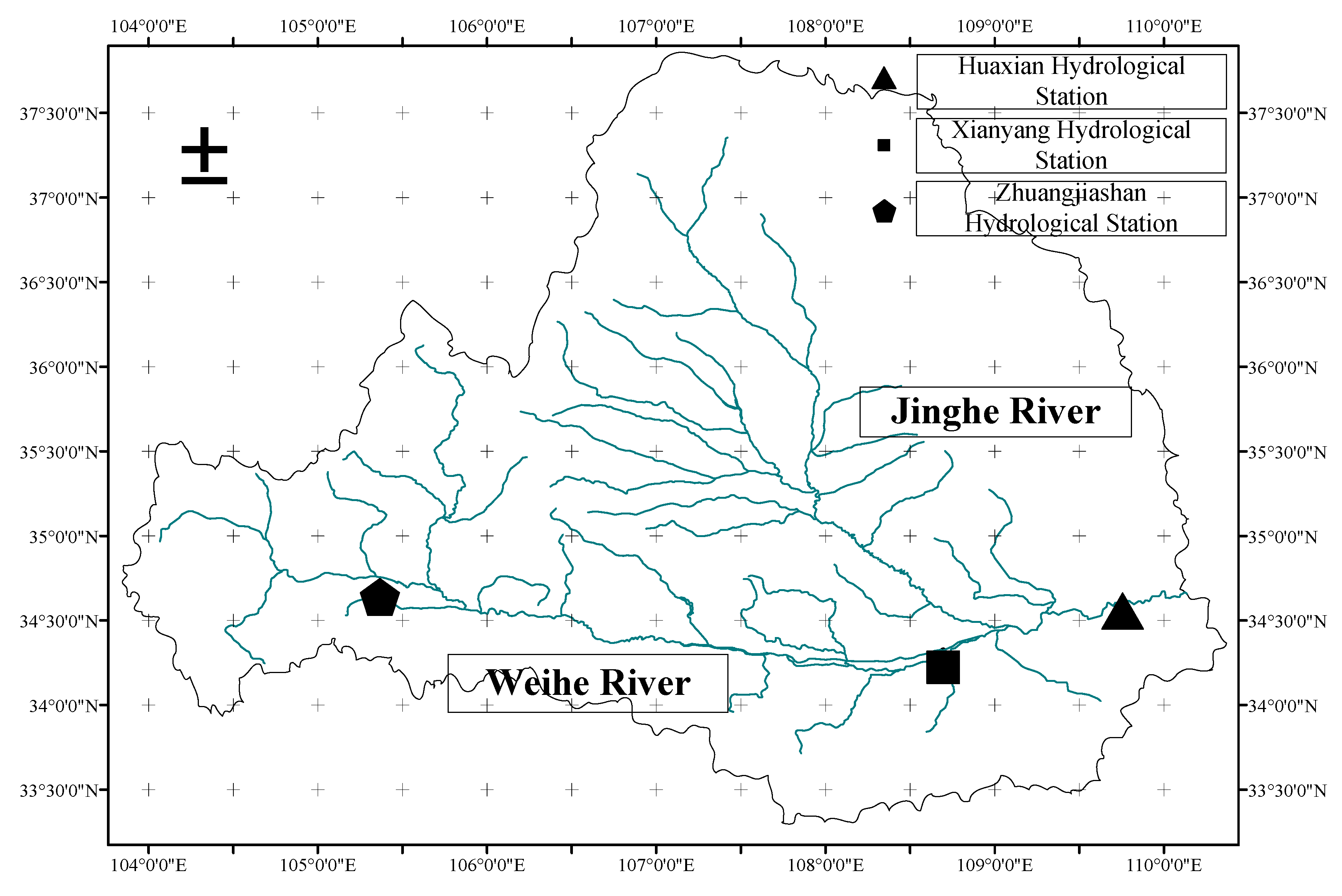
The Weihe River is the largest tributary of the Yellow River, and the Jinghe River is the largest tributary of the Weihe River. The Jinghe River originates from the Laolong Pond of Jingyuan County in the Ningxia Hui Autonomous Region, located at the eastern foot of the Liupan Mountain at an altitude of 2540 m. The Jinghe River flows from northwest to southeast through the Ningxia Hui Autonomous Region and the Gansu and Shaanxi provinces. Subsequently, it joins the Weihe River in Chenjiantan of Gaoling County in Shaanxi Province. The overall length of the mainstream is 455.10 km, and the drainage area is 45,421 km2. In this study, three reservoir sites comprising a multi-reservoirs system in the city of Weinan were considered: Xianyang, Huaxian County, and Zhangjiashan. The flood control standard of the urban and agricultural sections of Weinan city is once-in-a-century and once-in-half-a-century, respectively.
The Huaxian County reservoir has experienced 91 flood events with a daily flow rate greater than 1500 m3/s during 1960–2010. The related data of these cases were obtained through analyses of multiple representative reports on the regional watershed. The flood volume capacity of the Huaxian County site has sharply decreased, and its flood level has increased in recent years. This is primarily because the lower reaches of the Weihe River experienced severe sediment accumulation, and the riverbed has risen continuously since the construction of the Sanmenxia reservoir. For instance, the water level of the Huaxian County site in 2000 (1890 m3/s) was 0.27 m higher than in 1981 (5380 m3/s). At the Huaxian County site, the record level (occurring in 2003) was 0.15% higher than its second-highest level (occurring in 1996). Further, the historic peak water levels of the Xianyang and Huaxian County reservoirs were 5340 and 3570 m3/s, respectively. Therefore, the flood control situation is dire.
The Zhangjiashan future reservoir site and the Xianyang reservoir are 58 and 39 km away, respectively, from the Jinghe River estuary to the Weihe River. Therefore, flood risks at Zhangjiashan and Xianyang have high correlations with those in Huaxian County. One hydrological station has been established at each of the sites (Zhangjiashan, Xianyang, and Huaxian). The locations of hydrological stations along the Weihe River are shown in Figure 1.
3.2. Multi-Reservoir Joint Distribution and Data Collection
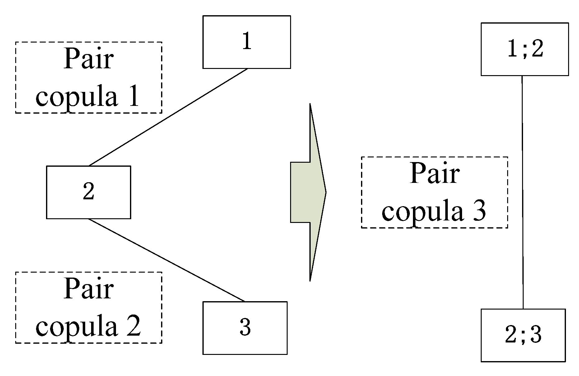
In this study, a joint flood risk distribution of the multi-reservoirs systems was constructed based on pair-copulas using vine construction. The related water conservancy data of the reservoirs were obtained through analyses of several reports on key water-control projects of the Jinghe River. The first pair-copula was built between Zhangjiashan and Xianyang. The interactive relationships among different components of the three reservoirs in the study area are shown in Figure 2.
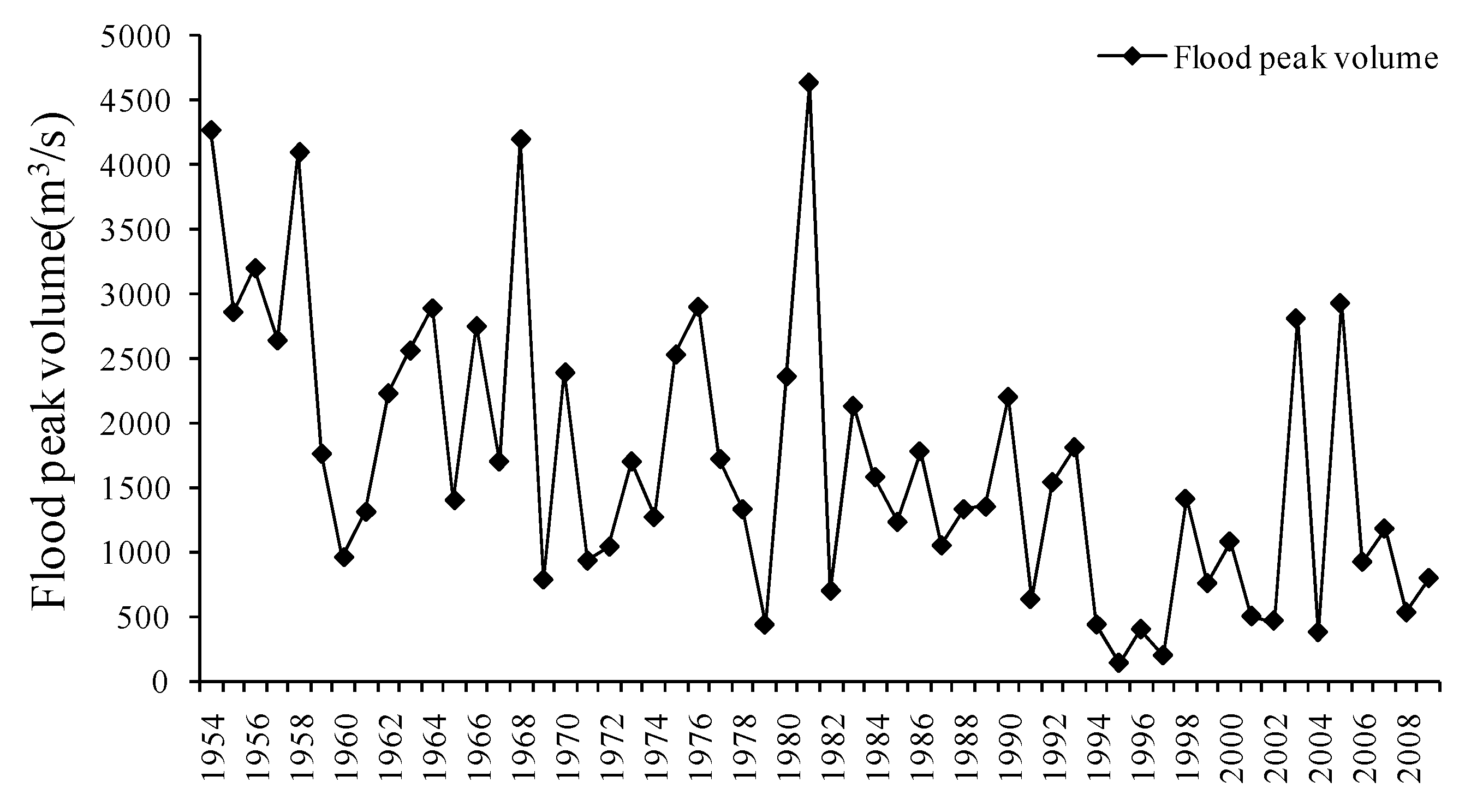
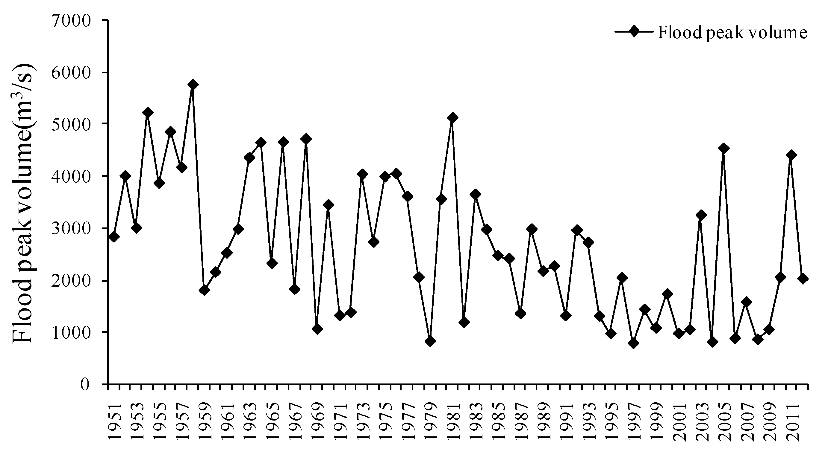
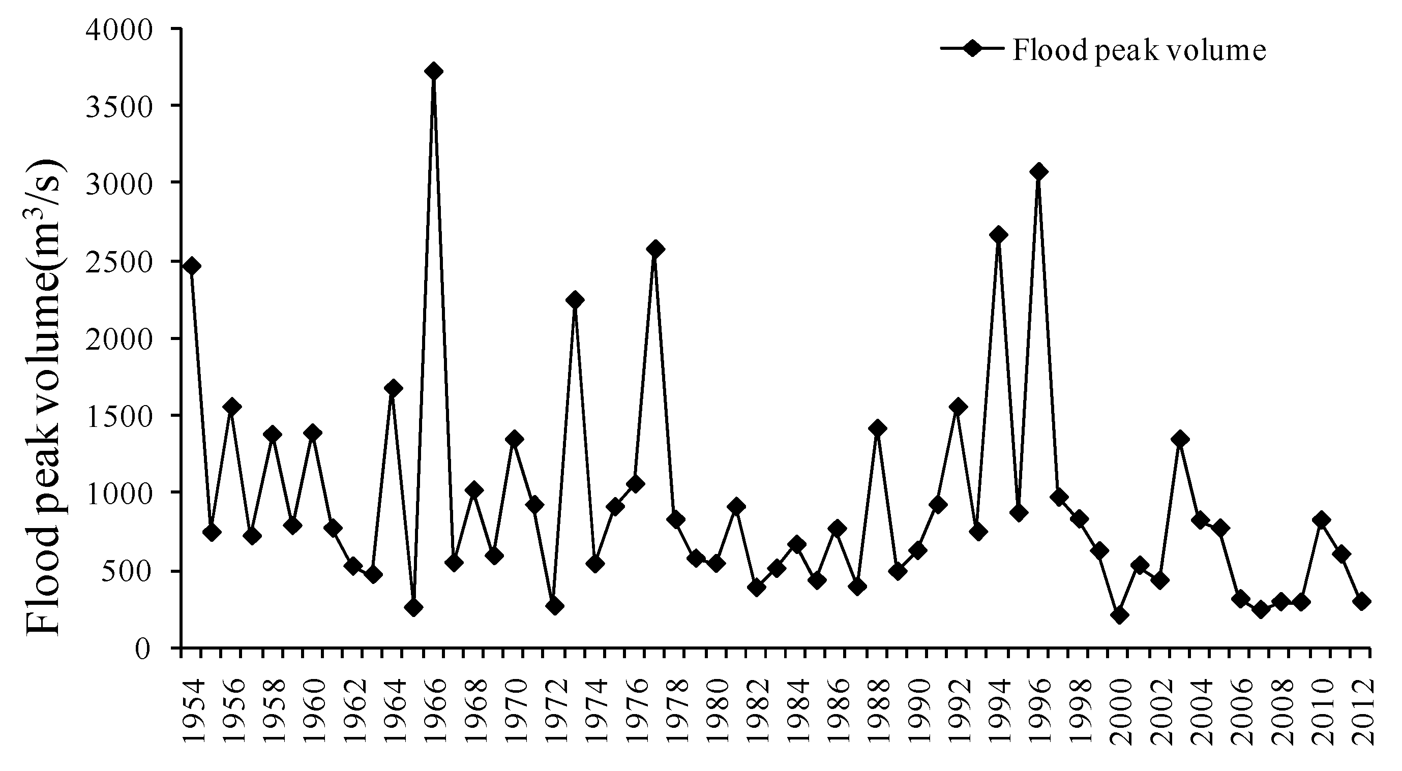
The flow data of the three sits are the foundation to establish the boundary function. Hydrological data were obtained from historical hydrological reports and the hydrological observation stations at Zhangjiashan, Xianyang, and Huaxian County. The flow data at Xianyang from 1953 to 2004 were obtained from historical hydrological reports of the Jinghe River, while 2005–2009 data were acquired from the aforementioned hydrological observation station. The flow data of Huaxian County from 1951 to 2004 were obtained from historical hydrological reports, while 2005–2012 data were from the hydrological observation station. Finally, Zhangjiashan flow data from 1954 to 2004 were obtained from historical hydrological reports, but 2005–2012 data were obtained from the hydrological observation station. Figure 3, Figure 4 and Figure 5 show the historical annual flood peak volume of the three sites. The flood peak volume of each hydrological observation station was also used to test the results.
4. Results and Discussion
In this study, 1-day, 3-day, 5-day, 9-day, 12-day, and flood peak volumes were considered and calculated. The minimum AIC and BIC volumes of copulas selected for the joint flood risk distribution are shown in Table 2. Reservoirs 1–3 represent Zhangjiashan, Xianyang, and Huaxian County, respectively. For instance, a Gaussian copula was selected for the 1-day volume of Zhangjiashan and Xianyang.
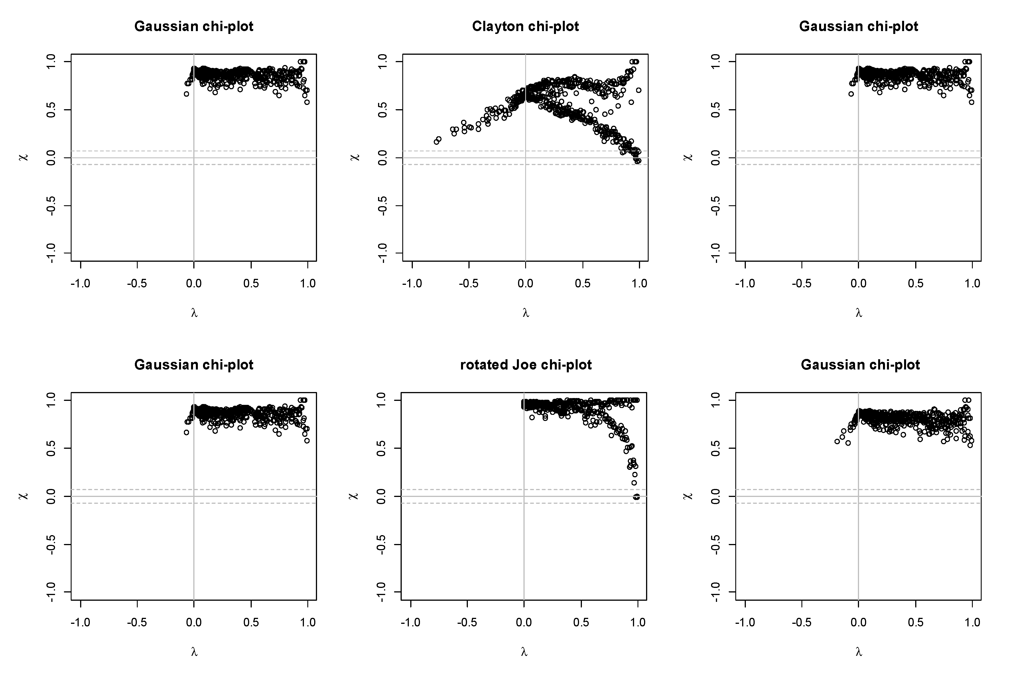
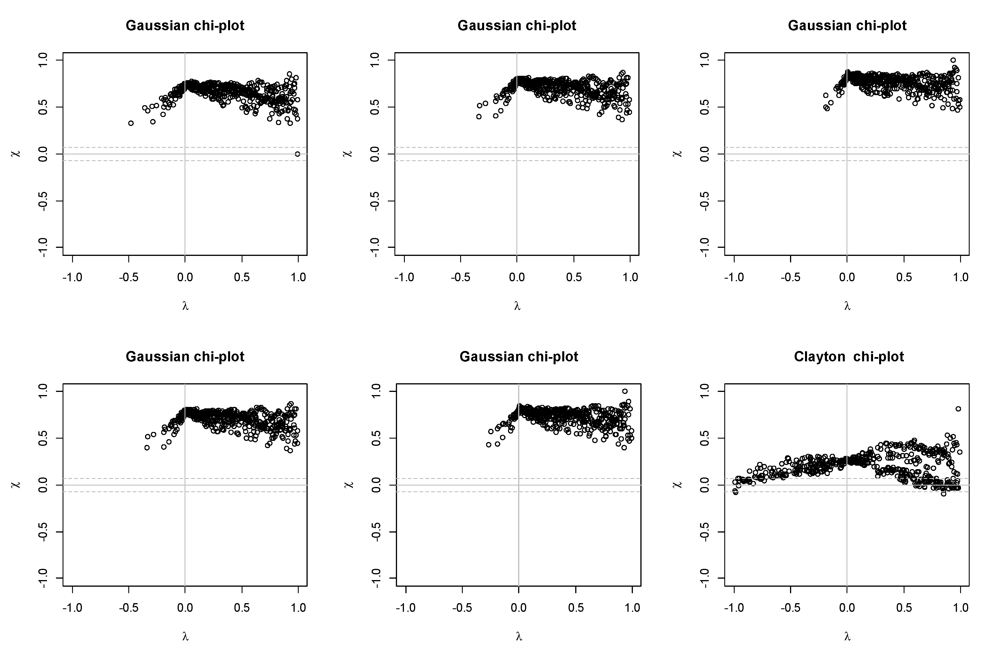
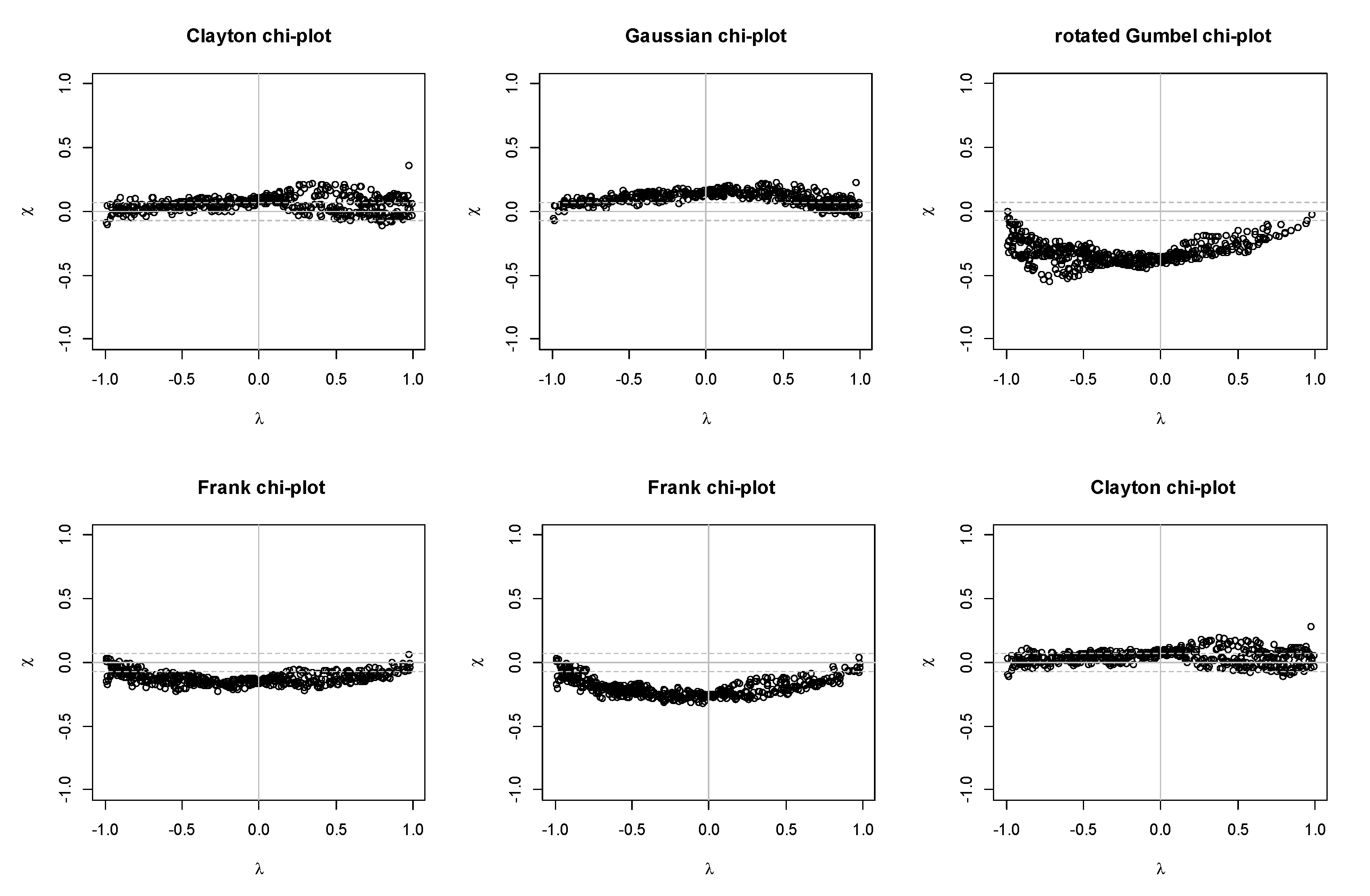
Figure 6, Figure 7 and Figure 8 show the chi-plots of pair flood volume variables. By analysing the pair dependency associations among the flood volumes of pair sites using graphical tools, such as chi-plots and K-plots, nonlinear data behaviour can be better ascertained than from a simple scatter plot. All points are random variables that obey the corresponding copula distribution. The data points are located above zero for positively dependent margins and below zero for negatively dependent margins.
Figure 6 shows the chi-plots of pair flood volume variables for Zhangjiashan and Xianyang (multi-reservoirs for 2,3). Random variables of the 1-day, 3-day, 5-day, 9-day, 12-day, and peak flood volumes obey the Gaussian, Clayton, Gaussian, Gaussian, Rotated Joe, and Gaussian distributions, respectively. It indicates that the 1-day, 3-day, 5-day, 9-day, 12-day, and flood peak volumes exhibit positive dependence.
Figure 7 shows the chi-plots of pair flood volume variables for Xianyang and Huaxian County (multi-reservoirs for 1,2). Random variables of the 1-day, 3-day, 5-day, 9-day, 12-day, and peak flood volumes obey the Gaussian, Gaussian, Gaussian, Gaussian, Gaussian, and Clayton distributions, respectively. The 1-day, 3-day, 5-day, 9-day, 12-day, and flood peak volumes also exhibit positive dependence. In addition, the peak flood volume shows a weakly positive dependence.
Finally, Figure 8 shows the chi-plots of pair flood volume variables for Zhangjiashan and Huaxian County (multi-reservoirs for 1,3:2). Random variables of the 1-day, 3-day, 5-day, 9-day, 12-day, and peak flood volumes obey the Clayton, Gaussian, Rotated Gumbel, Frank, Frank, and Clayton distributions, respectively. It indicates that the 1-day, 3-day, and flood peak flood volumes are independent. However, the 5-day, 9-day, and 12-day flood volumes exhibit weak negative dependence.
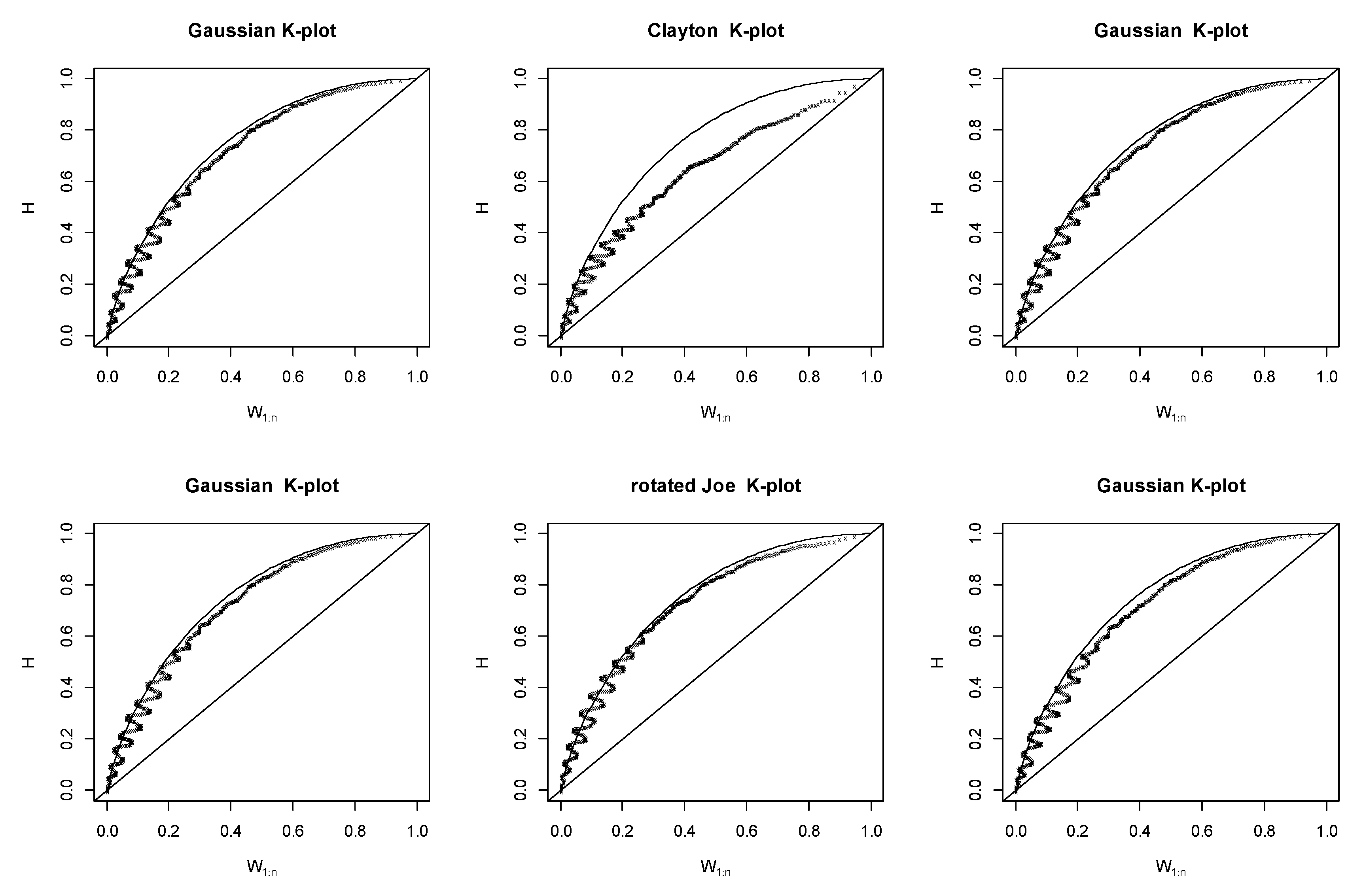
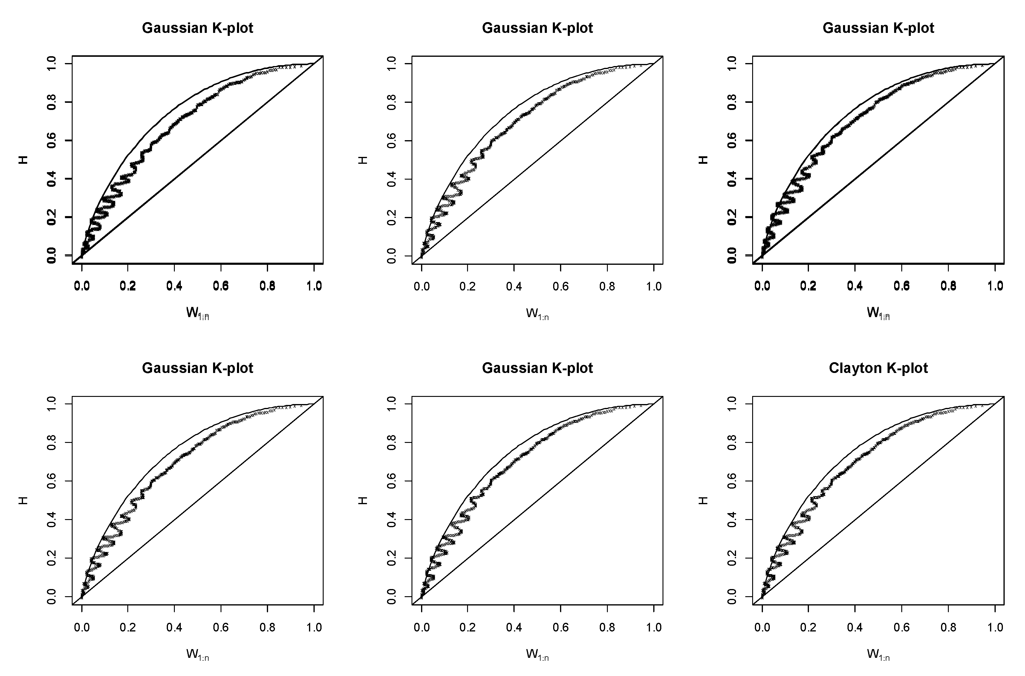
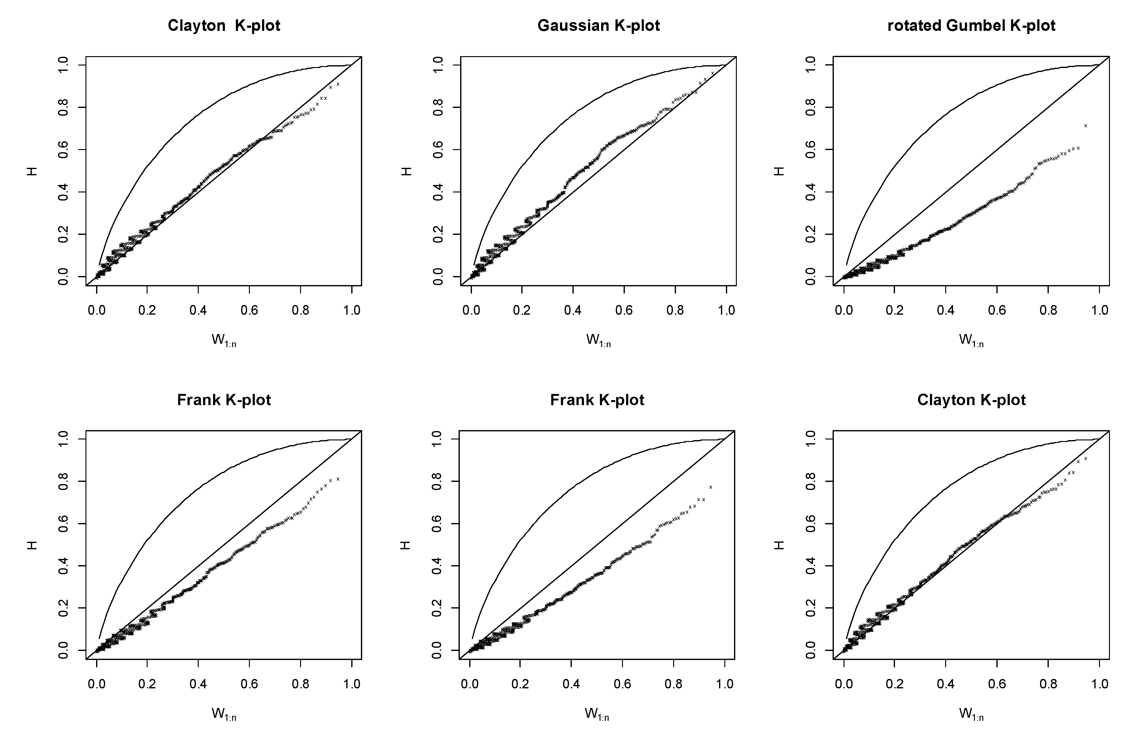
Figure 9, Figure 10 and Figure 11 present the K-plots of pair flood volume variables. All points are also random variables that obey the corresponding copula distribution. Figure 9 shows the K-plots of pair flood volume variables for Zhangjiashan and Xianyang (multi-reservoirs for 2,3). Random variables of the 1-day, 3-day, 5-day, 9-day, 12-day, and peak flood volumes obey the Gaussian, Clayton, Gaussian, Gaussian, Rotated Joe, and Gaussian distributions, respectively. A deviation is observed from the centre of the main diagonal, indicating a positive association between the two sites. Figure 10 shows a positive association between Xianyang and Huaxian County (multi-reservoirs for 1,2). Random variables of the 1-day, 3-day, 5-day, 9-day, 12-day, and peak flood volumes obey the Gaussian, Gaussian, Gaussian, Gaussian, Gaussian, and Clayton distributions, respectively. Random variables of the 1-day, 3-day, 5-day, 9-day, 12-day, and flood peak volumes exhibit positive dependence. From Figure 11, the K-plots of pair flood volume variables for Zhangjiashan and Huaxian County (multi-reservoirs for 1,3:2) indicate that the 1-day, 3-day, and flood peak volumes (Clayton, Gaussian, Rotated Gumbel, Frank, Frank, and Clayton distributions, respectively) are independent. However, the 5-day, 9-day, and 12-day flood volumes exhibit negative dependence. These results demonstrate that some risks from Huaxian County would transfer to Xianyang and Zhangjiashan. Therefore, Xianyang shares more risks with Huaxian County than Zhangjiashan.
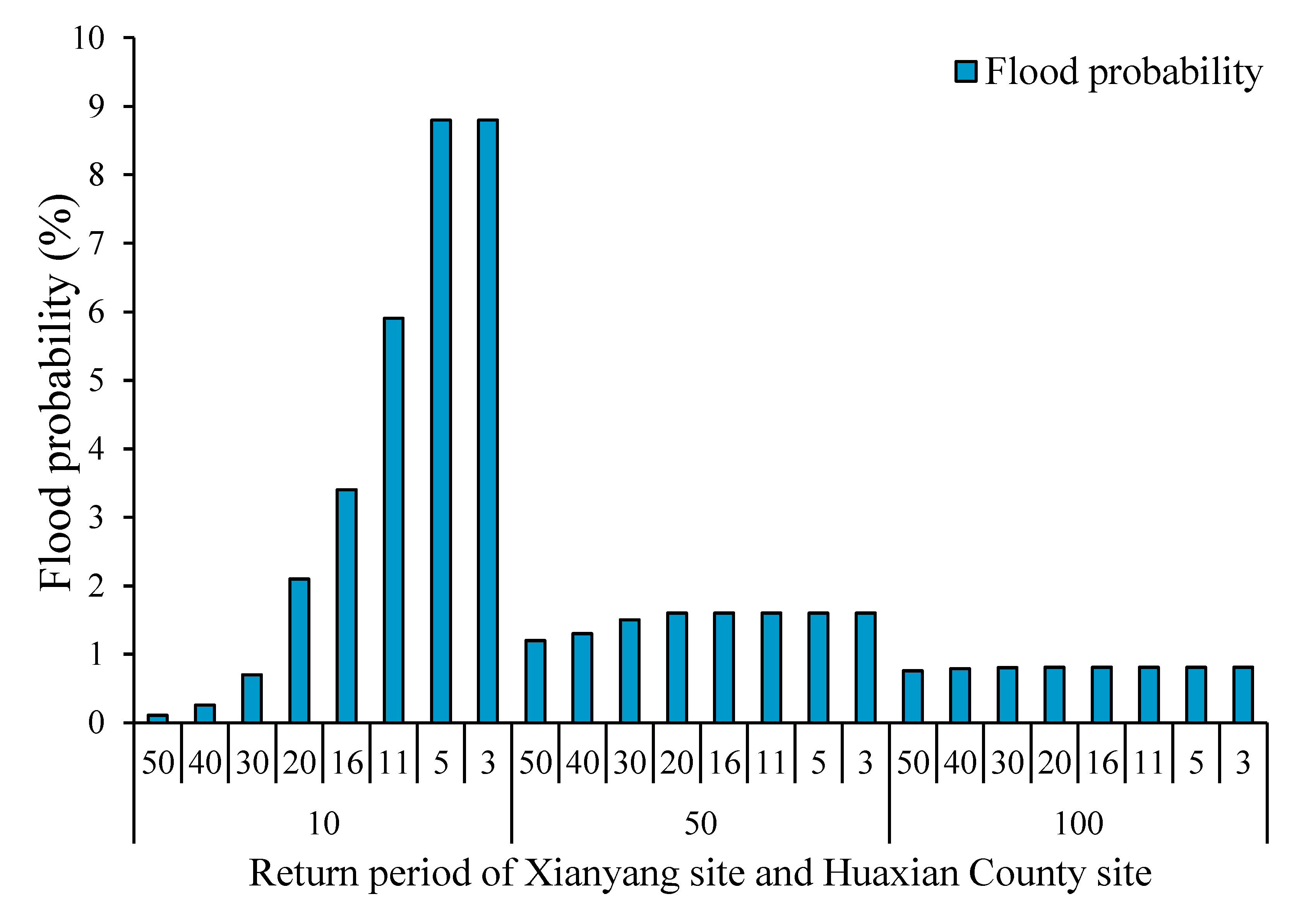
The KGE value of Zhangjiashan and Huaxian County under various return periods at Xianyang are shown in Table 3. They suggest that the imitative effects are satisfactory for validation. The flood risk and corresponding flood volume of Zhangjiashan were calculated for various flood risk levels of Xianyang and Huaxian County using the joint flood risk distribution. Table 4 and Table 5 present the calculated flood volume of Zhangjiashan, while Figure 12 shows the calculated flood probability for Zhangjiashan. The flood probability of Zhangjiashan increased with the flood risk of Huaxian County, reducing the 10-year return period of Xianyang. For instance, the flood probability of Zhangjiashan was 0.11%, 0.26%, 0.7%, 2.1%, 3.4%, 5.9%, 8.8%, and 8.8% in the 50-year, 40-year, 30-year, 20-year, 16-year, 11-year, 5-year, and 3-year return periods, respectively, at Huaxian County, showing a progressive decrease from 50-year to 3-year return periods. These results indicate that the flood risk of Zhangjiashan would decrease along with that of Huaxian County under a small return period at Xianyang. Moreover, Zhangjiashan would assume a high flood risk from Huaxian County to maintain the low flood risk of Xianyang.
In contrast, the flood risk of Zhangjiashan would not change with decreases in flood risk within Huaxian County under 50-year flooding (i.e., flooding with a 50-year return period) in Xianyang. For instance, the flood probability of Zhangjiashan was stable for the 50-year return period at Xianyang with the flood probability at Zhangjiashan being 1.2%, 1.3%, 1.5%, 1.6%, 1.6%, 1.6%, 1.6%, and 1.6% in the 50-year, 40-year, 30-year, 20-year, 16-year, 11-year, 5-year, and 3-year return periods, respectively, at Huaxian County. These results demonstrate that the most dynamic flood risks in Huaxian County were observed at Zhangjiashan. Therefore, Zhangjiashan would continue to exhibit a high flood risk because of the large flood risk at the other two sites. Moreover, the flood probability at Zhangjiashan exhibited stability for the 100-year return period at Xianyang. Thus, Zhangjiashan retained a high flood risk because of Xianyang.
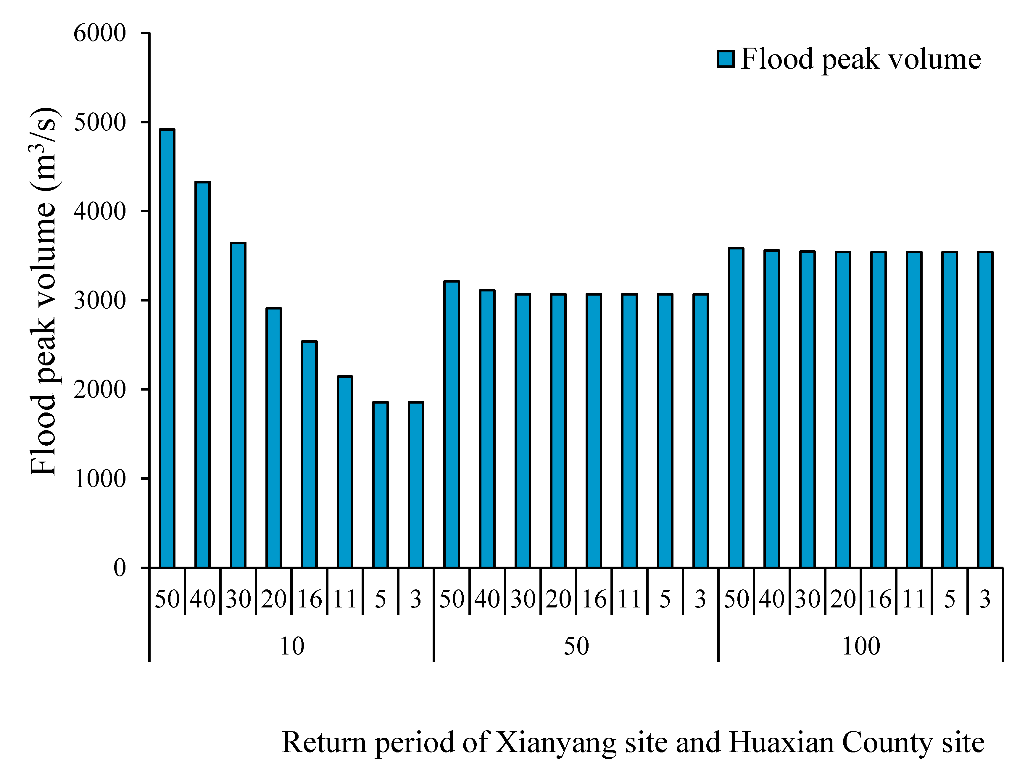
The flood volume of Zhangjiashan was calculated based on its flood probability. Figure 13 shows the calculated flood peak volume of Zhangjiashan under various return periods in Xianyang and Huaxian County. The flood volume of Zhangjiashan corresponded to its flood risk levels, with the flood peak volume being 4915, 4325, 3541, 2909, 2536, 2144, 1856, and 1856 m3/s in the 50-year, 40-year, 30-year, 20-year, 16-year, 11-year, 5-year, and 3-year return periods, respectively, in Huaxian County. Therefore, Zhangjiashan would face high flood risks from Huaxian County to maintain the low flood risk of Xianyang. Moreover, a small probability event at Zhangjiashan could occur when Xianyang has a low flood risk. However, Huaxian County was found to be at a high flood risk. Zhangjiashan would only have a low flood risk when Xianyang and Huaxian Country also show low flood risks.
The flood peak volume of Zhangjiashan was stable for the 50-year return period at Xianyang. The flood volume of Zhangjiashan was 3211, 3110, 3066, 3066, 3066, 3066, 3066, and 3066 m3/s in the 50-year, 40-year, 30-year, 20-year, 16-year, 11-year, 5-year, and 3-year return periods, respectively, at Huaxian County. This result indicates that Zhangjiashan would not share risks when the flood risk of Xianyang is lower than the low flood risk of Huaxian County. Therefore, the flood risk of Xianyang has little influence on the flood risk of Zhangjiashan. For example, the flood peak volume of Zhangjiashan was 2909, 3066, and 3540 m3/s for the 20-year return period at Huaxian County in the 10-year, 50-year, and 10-year return periods, respectively, at Xianyang. These results correspond to the relative geographic positions of Xianyang and Zhangjiashan.
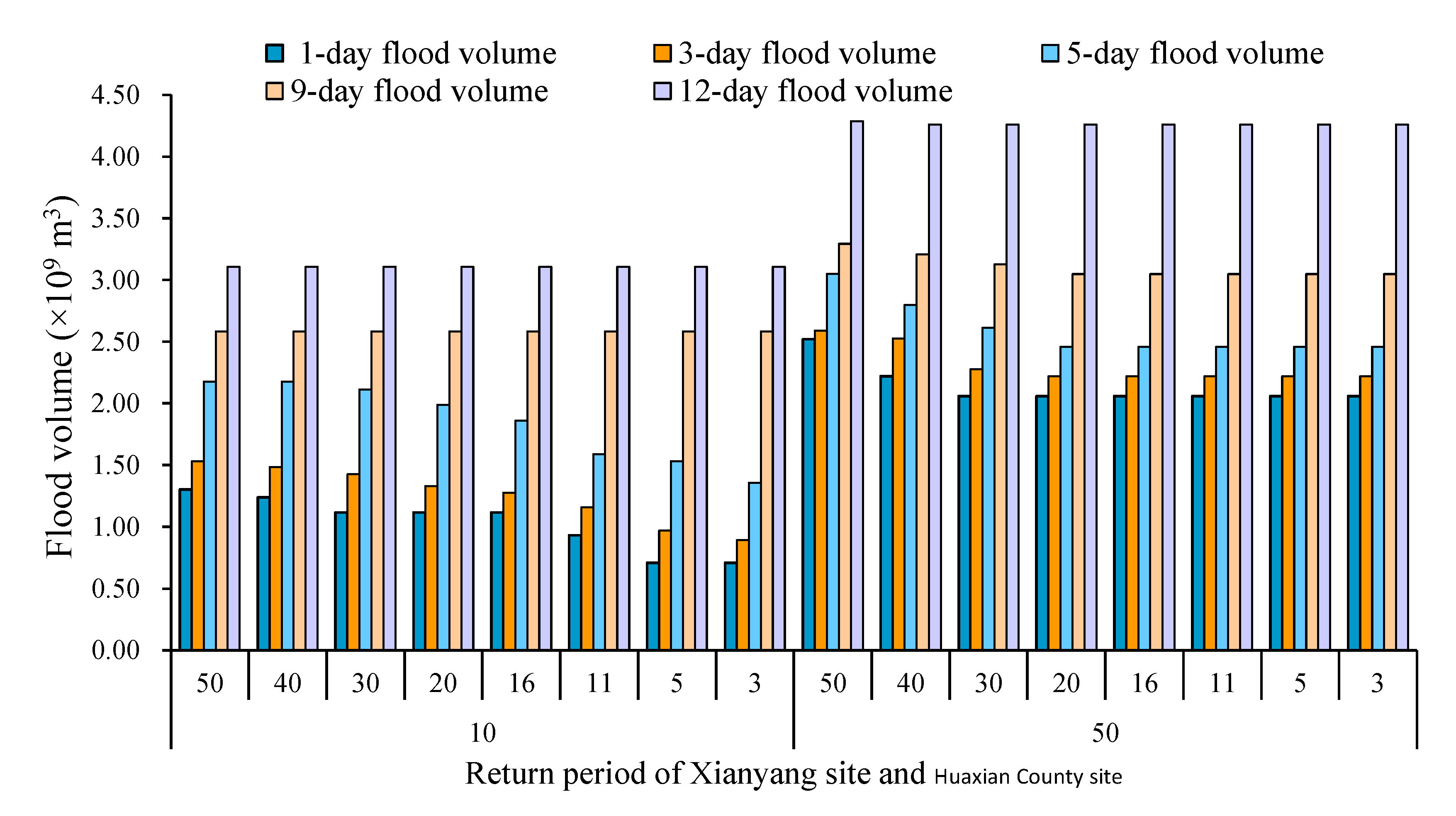
Figure 14 presents the 1-day, 3-day, 5-day, 9-day, and 12-day flood volumes of Zhangjiashan under various return periods at Xianyang and Huaxian County. The 1-day flood volume of Zhangjiashan corresponded to its flood risk levels with the flood peak volume at 1.30 × 10⁹, 1.24 × 10⁹, 1.12 × 10⁹, 1.12 × 10⁹, 1.12 × 10⁹, 0.93 × 10⁹, 0.71 × 10⁹, and 0.71 × 10⁹ m3 in the 50-year, 40-year, 30-year, 20-year, 16-year, 11-year, 5-year, and 3-year return periods, respectively, at Huaxian County. Moreover, the 1-day, 3-day, and 5-day flood volumes would be similar to the flood peak volume of Zhangjiashan. In contrast, the 9-day and 12-day flood volumes showed fewer variations with different risk levels at the Huaxian County site. Therefore, the long-term cumulative flood volume was strongly related to other regions that shared similar risks.
5. Conclusions
In conclusion, using a real-world case study, the flood risk transfer in a multi-reservoir system was analysed. A copula-based approach was developed to construct the joint flood risk distribution of multi-reservoirs. This approach provided a practical and straightforward scheme to structure high-dimensional probability functions from multivariate sample flood volumes of hydrological stations. K-plots and chi-plots were generated to analyse correlations between reservoirs. Further, multi-reservoirs in the Weihe River drainage tributary included three reservoir sites: Xianyang, Huaxian County, and Zhangjiashan. It was determined that the risks of Huaxian County would be transferred to Xianyang and Zhangjiashan to some extent. Moreover, Xianyang would mitigate comparatively more flood risks from Huaxian County than from Zhangjiashan.
The flood risk and corresponding flood volume of Zhangjiashan were calculated for various flood risk levels in Xianyang and Huaxian County using joint flood risk distribution. For example, the flood peak volume of Zhangjiashan was only 1856 m3 during the 10-year return period at Xianyang and the 5-year return period at Huaxian County. The complex relationship among the flood volumes of the three reservoirs was also analysed. The study results provide constructive suggestions for the Zhangjiashan reservoir construction project. Furthermore, the flood risk distribution of multi-reservoirs using a copula-based approach can provide new insights into reservoir joint disposal and risk control. However, there are many factors and indicators that pertain to reservoir construction (e.g., sediment amount, regional rainfall). Integrating these factors and indicators into a copula-based approach presents an interesting potential avenue for future research.
Author Contributions
Conceptualization, S.W. (Shen Wang); Methodology, S.W. (Shen Wang); Software, S.W. (Shen Wang), J.W. and S.W. (Siyi Wang); Validation, S.W. (Shen Wang), X.X., Y.F. and L.L.; Formal analysis, S.W. (Shen Wang), L.L. and G.H.; Investigation, S.W. (Shen Wang) and J.W.; Resources, S.W. (Shen Wang), L.L. and G.H.; Data curation, J.W. and S.W. (Siyi Wang); Writing—original draft preparation, S.W. (Shen Wang); Visualization, S.W. (Shen Wang); Supervision, Y.F.; Project administration, L.L.; Funding acquisition, L.L. All authors have read and agreed to the published version of the manuscript.
Funding
This research was funded by the Fundamental Research Funds for Public Welfare Research Institutes of the Chinese Research Academy of Environmental Sciences, grant number 2021-JY-29.
Data Availability Statement
Not applicable.
Acknowledgments
The authors are grateful to the reviewers and editors for their valuable comments and suggestions.
Conflicts of Interest
The authors declare no conflict of interest.
References
- Rauter, M.; Thaler, T.; Attems, M.-S.; Fuchs, S. Obligation or Innovation: Can the EU Floods Directive Be Seen as a Tipping Point Towards More Resilient Flood Risk Management? A Case Study From Vorarlberg, Austria. Sustainability 2019, 11, 5505. [Google Scholar] [CrossRef]
- Obeidat, M.; Awawdeh, M.; Al-Hantouli, F. Morphometric Analysis and Prioritisation of Watersheds for Flood Risk Management in Wadi Easal Basin (WEB), Jordan, Using Geospatial Technologies. J. Flood Risk Manag. 2021, 14, e12711. [Google Scholar] [CrossRef]
- Pangali Sharma, T.P.; Zhang, J.; Khanal, N.R.; Prodhan, F.A.; Nanzad, L.; Zhang, D.; Nepal, P. A Geomorphic Approach for Identifying Flash Flood Potential Areas in the East Rapti River Basin of Nepal. ISPRS Int. J. Geo Inf. 2021, 10, 247. [Google Scholar] [CrossRef]
- Seleem, O.; Heistermann, M.; Bronstert, A. Efficient Hazard Assessment for Pluvial Floods in Urban Environments: A Benchmarking Case Study for the City of Berlin, Germany. Water 2021, 13, 2476. [Google Scholar] [CrossRef]
- Jin, S.Y.; Guo, S.M.; Huo, W.H. Analysis on the Return Period of “7.20” Rainstorm in the Xiaohua Section of the Yellow River in 2021. Water 2022, 14, 2444. [Google Scholar] [CrossRef]
- Chen, F.L.; Zheng, J.T.; Li, S.F.; Long, A.H. Effects of the Land Use and Check Dams on Flood in Upper Catchment of Fuping Hydrological Station by Hydrological Modeling. Water Resour. 2018, 45, 508–522. [Google Scholar] [CrossRef]
- El-Rawy, M.; Elsadek, W.M.; De Smedt, F.D. Flash Flood Susceptibility Mapping in Sinai, Egypt Using Hydromorphic Data, Principal Component Analysis and Logistic Regression. Water 2022, 14, 2434. [Google Scholar] [CrossRef]
- Tanim, A.H.; McRae, C.B.; Tavakol-Davani, H.; Goharian, E. Flood Detection in Urban Areas Using Satellite Imagery and Machine Learning. Water 2022, 14, 1140. [Google Scholar] [CrossRef]
- Zhou, Z.; Smith, J.A.; Wright, D.B.; Baeck, M.L.; Yang, L.; Liu, S. Storm Catalog-Based Analysis of Rainfall Heterogeneity and Frequency in a Complex Terrain. Water Resour. Res. 2019, 55, 1871–1889. [Google Scholar] [CrossRef]
- Prairie, J.; Rajagopalan, B.; Lall, U.; Fulp, T. A Stochastic Nonparametric Technique for Space-Time Disaggregation of Streamflows. Water Resour. Res. 2007, 43, W03432. [Google Scholar] [CrossRef] [Green Version]
- Hao, Z.; Singh, V.P. Modeling Multisite Streamflow Dependence With Maximum Entropy Copula. Water Resour. Res. 2013, 49, 7139–7143. [Google Scholar] [CrossRef]
- Chen, L.; Singh, V.P.; Guo, S.; Zhou, J.; Zhang, J. Copula-Based Method for Multisite Monthly and Daily Streamflow Simulation. J. Hydrol. 2015, 528, 369–384. [Google Scholar] [CrossRef]
- Krstanovic, P.F.; Singh, V.P. A Multivariate Stochastic Flood Analysis Using Entropy. In Hydrologic Frequency Modeling; Singh, V.P., Ed.; Reidel: Dordrecht, The Netherlands, 1987; pp. 515–539. [Google Scholar]
- Yue, S. The Bivariate Lognormal Distribution to Model a Multi Variate Flood Episode. Hydrol. Process. 2000, 14, 2575–2588. [Google Scholar] [CrossRef]
- Escalante-Sandoval, C. Application of Bivariate Extreme Value Distribution to Flood Frequency Analysis: A Case Study of Northwestern Mexico. Nat. Hazards. 2007, 42, 37–46. [Google Scholar] [CrossRef]
- Sandoval, C.E.; Raynal-Villaseñor, J. Trivariate Generalized Extreme Value Distribution in Flood Frequency Analysis. Hydrol. Sci. J. 2008, 53, 550–567. [Google Scholar] [CrossRef]
- Grimaldi, S.; Serinaldi, F. Asymmetric Copula in Multivariate Flood Frequency Analysis. Adv. Water Resour. 2006, 29, 1155–1167. [Google Scholar] [CrossRef]
- Zhang, L.; Singh, V.P. Trivariate Flood Frequency Analysis Using the Gumbel–Hougaard Copula. J. Hydrol. Eng. 2007, 12, 431–439. [Google Scholar] [CrossRef]
- Pinya, M.A.S.; Madsen, H.; Rosbjerg, D. Assessment of the Risk of Inland Flooding in a Tidal Sluice Regulated Catchment Using Multi-variate Statistical Techniques. Phys. Chem. Earth Parts A B C 2009, 34, 662–669. [Google Scholar] [CrossRef]
- Salvadori, G.; De Michele, C. Frequency Analysis via Copulas: Theoretical Aspects and Applications to Hydrological Events. Water Resour. Res. 2004, 40, 12. [Google Scholar] [CrossRef]
- Karmakar, S.; Simonovic, S.P. Bivariate Flood Frequency Analysis. Part 2: A Copula-Based Approach With Mixed Marginal Distributions. J. Flood Risk Manag. 2009, 2, 32–44. [Google Scholar] [CrossRef]
- Latif, S.; Mustafa, F. Copula-Based Multivariate Flood Probability Construction: A Review. Arab. J. Geosci. 2020, 13, 132. [Google Scholar] [CrossRef]
- Zhong, M.; Zeng, T.; Jiang, T.; Wu, H.; Hong, Y. A Copula-Based Multivariate Probability Analysis for Flash Flood Risk Under the Compound Effect of Soil Moisture and Rainfall. Water Resour. Manag. 2021, 35, 83–98. [Google Scholar] [CrossRef]
- Bárdossy, A.; Pegram, G.G.S. Copula Based Multisite Model for Daily Precipitation Simulation. Hydrol. Earth Syst. Sci. 2009, 13, 2299–2314. [Google Scholar] [CrossRef]
- Requena, A.I.; Mediero, L.; Garrote, L. A Bivariate Return Period Based on Copulas for Hydrologic Dam Design: Accounting for Reservoir Routing in Risk Estimation. Hydrol. Earth Syst. Sci. 2013, 17, 3023–3038. [Google Scholar] [CrossRef]
- Sancetta, A.; Satchell, S. The Bernstein Copula and Its Applications to Modeling and Approximations of Multivariate Distributions. Econ. Theory. 2004, 20, 535–562. [Google Scholar] [CrossRef]
- Tang, X.S.; Li, D.Q.; Zhou, C.B.; Zhang, L.M. Bivariate Distribution Models Using Copulas for Reliability Analysis. Proc. Inst. Mech. Eng. O. 2013, 227, 499–512. [Google Scholar] [CrossRef]
- Tao, S.; Dong, S.; Wang, N.; Guedes Soares, C.G. Estimating Storm Surge Intensity With Poisson Bivariate Maximum Entropy Distributions Based on Copulas. Nat. Hazards. 2013, 68, 791–807. [Google Scholar] [CrossRef]
- Nelsen, R.B. An Introduction to Copulas; Springer: New York, NY, USA, 2006. [Google Scholar]
- Aas, K.; Czado, C.; Frigessi, A.; Bakken, H. Pair-Copula Constructions of Multiple Dependence. Ins. Math. Econ. 2009, 44, 182–198. [Google Scholar] [CrossRef]
- Chen, Q.P. A Study on Pair-Copula Constructions of Multiple Dependence. Appl. Stat. Manag. 2013, 44, 182–198. [Google Scholar]
- Sklar, A. Random Variables, Distribution Functions, and Copulas: A Personal Look Backward and Forward. Lect. Notes-Monograph. 1996, 28, 1–14. [Google Scholar]
- Akaike, H. Information Theory as an Extension of the Maximum Likelihood Principle. In Second International Symposium on Information Theory; Petrov, B.N., Csaki, F., Eds.; Akadémiai Kiadó: Budapest, Hungary, 1973; pp. 276–281. [Google Scholar]
- Banks, H.T.; Joyner, M.L. AIC Under the Framework of Least Squares Estimation. Appl. Math. Lett. 2017, 74, 33–45. [Google Scholar] [CrossRef]
- Bozdogan, H. Model Selection and Akaike’s Information Criterion (AIC): The General Theory and Its Analytical Extensions. Psychometrika 1987, 52, 345–370. [Google Scholar] [CrossRef]
- Hamed, M.M.; Nashwan, M.S.; Shahid, S.; Ismail, T.B.; Wang, X.J.; Dewan, A.; Asaduzzaman, M. Inconsistency in historical simulations and future projections of temperature and rainfall: A comparison of CMIP5 and CMIP6 models over Southeast Asia. Atmos. Res. 2022, 265, 105927. [Google Scholar] [CrossRef]
- Nashwan, M.S.; Shahid, S. A novel framework for selecting general circulation models based on the spatial patterns of climate. Int. J. Climatol. 2020, 40, 4422–4443. [Google Scholar] [CrossRef]
Figure 1.
Location of hydrological stations in Weihe River.

Figure 2.
Diagram of three reservoir pair-copulas with canonical-vine structure.

Figure 3.
Annual flood peak volume of Xianyang from 1954 to 2008.

Figure 4.
Annual flood peak volume of Huaxian County from 1951 to 2012.

Figure 5.
Annual flood peak volume of Zhangjiashan from 1951 to 2012.

Figure 6.
Chi-plots of pair flood volume variables of Zhangjiashan and Xianyang.

Figure 7.
Chi-plots of pair flood volume variables of Xianyang and Huaxian County.

Figure 8.
Chi-plots of pair flood volume variables of Zhangjiashan and Huaxian County.

Figure 9.
K-plots of pair flood volume variables of Zhangjiashan and Xianyang.

Figure 10.
K-plots of pair flood volume variables of Xianyang and Huaxian County.

Figure 11.
K-plots of pair flood volume variables of Zhangjiashan and Huaxian County.

Figure 12.
Flood probability of Zhangjiashan under different return periods of Xianyang and Huaxian County.
Figure 12.
Flood probability of Zhangjiashan under different return periods of Xianyang and Huaxian County.

Figure 13.
Flood peak volume of Zhangjiashan under different return periods of Xianyang and Huaxian County.
Figure 13.
Flood peak volume of Zhangjiashan under different return periods of Xianyang and Huaxian County.

Figure 14.
Flood volume of Zhangjiashan under different return periods of Xianyang and Huaxian County.
Figure 14.
Flood volume of Zhangjiashan under different return periods of Xianyang and Huaxian County.


Table 1.
Archimedean copula functions.
| Copula | Generating Function | Parameter | |
|---|---|---|---|
| Gumbel copula | [1, ∞) | ||
| Clayton copula | (0, ∞) | ||
| Frank copula | R |
Note: where u and v are the marginal distributions, and φ is the generating function.
Table 2.
Selected copulas for multi-reservoir joint flood risk distribution with minimum AIC and BIC.
Table 2.
Selected copulas for multi-reservoir joint flood risk distribution with minimum AIC and BIC.
| Multi-Reservoirs | Chosen Copula | AIC | BIC | |
|---|---|---|---|---|
| 1-day volume | 1,2 | Gaussian | −4372.627 | −4356.78 |
| 2,3 | Gaussian | −13,322.1 | −13,314.2 | |
| 1,3:2 | Clayton | −40,068.585 | −40,060.7 | |
| Full | −10,036.55 | −10,023.8 | ||
| 3-day volume | 1,2 | Gaussian | −5542.449 | −5526.6 |
| 2,3 | Clayton | −13,780.09 | −13,772.2 | |
| 1,3:2 | Gaussian | −43,701.22 | −43,693.3 | |
| Full | −11,746.95 | −11,734.2 | ||
| 5-day volume | 1,2 | Gaussian | −6262.168 | −6246.32 |
| 2,3 | Gaussian | −14,147.22 | −14,139.3 | |
| 1,3:2 | Rotated Gumbel | −45,910.489 | −45,902.6 | |
| Full | −12,766.7 | −12,754 | ||
| 9-day volume | 1,2 | Gaussian | −7023.314 | −7007.46 |
| 2,3 | Gaussian | −14,858.63 | −14,850.7 | |
| 1,3:2 | Frank | −48,641.955 | −48,634 | |
| Full | −12,603.55 | −12,590.8 | ||
| 12-day volume | 1,2 | Gaussian | −7376.352 | −7360.5 |
| 2,3 | Rotated Joe | −15,311.32 | −15,303.4 | |
| 1,3:2 | Frank | −49,965.467 | −49,957.5 | |
| Full | −303,895.2 | −303,883 | ||
| Flood peak volume | 1,2 | Clayton | −4372.627 | −4356.78 |
| 2,3 | Gaussian | −13,322.1 | −13,314.2 | |
| 1,3:2 | Clayton | −40,068.585 | −40,060.7 | |
| Full | −3546.92 | −3534.21 |
Table 3.
KGE values of Zhangjiashan and Huaxian County under various return periods at Xianyang.
| Return Period of Xianyang Site | ||||||||
|---|---|---|---|---|---|---|---|---|
| 50 | 40 | 30 | 20 | 16 | 11 | 5 | 3 | |
| Flood peak volume | 0.242 | 0.265 | 0.315 | 0.351 | 0.235 | 0.138 | 0.175 | 0.108 |
| 1-day flood volumes | 0.012 | 0.090 | 0.359 | 0.321 | 0.283 | 0.168 | 0.051 | 0.012 |
| 3-day flood volumes | 0.059 | 0.164 | 0.253 | 0.278 | 0.130 | 0.059 | 0.095 | 0.021 |
| 5-day flood volumes | 0.012 | 0.090 | 0.359 | 0.321 | 0.283 | 0.168 | 0.051 | 0.012 |
| 9-day flood volumes | 0.169 | 0.106 | 0.042 | 0.029 | 0.016 | 0.010 | 0.029 | 0.042 |
| 12-day flood volumes | 0.160 | 0.097 | 0.033 | 0.021 | 0.008 | 0.002 | 0.021 | 0.033 |
Table 4.
Flood peak volume of Zhangjiashan under different return periods of Xianyang and Huaxian County.
Table 4.
Flood peak volume of Zhangjiashan under different return periods of Xianyang and Huaxian County.
| Return Period | Flood Peak Volume (m3/s) | |
|---|---|---|
| Xianyang | Huaxian County | Zhangjiashan |
| 10 | 50 | 4915 |
| 40 | 4325 | |
| 30 | 3641 | |
| 20 | 2909 | |
| 16 | 2536 | |
| 11 | 2144 | |
| 5 | 1856 | |
| 3 | 1856 | |
| 50 | 50 | 3211 |
| 40 | 3110 | |
| 30 | 3066 | |
| 20 | 3066 | |
| 16 | 3066 | |
| 11 | 3066 | |
| 5 | 3066 | |
| 3 | 3066 | |
| 100 | 50 | 3583 |
| 40 | 3558 | |
| 30 | 3547 | |
| 20 | 3540 | |
| 16 | 3540 | |
| 11 | 3540 | |
| 5 | 3540 | |
| 3 | 3540 | |
Table 5.
Flood volume of Zhangjiashan under different return periods of Xianyang and Huaxian County.
Table 5.
Flood volume of Zhangjiashan under different return periods of Xianyang and Huaxian County.
| Return Period | Flood Volume (m3) | |||||
|---|---|---|---|---|---|---|
| Xianyang | Huaxian County | Zhangjiashan Site | ||||
| 10 | 50 | 15,080 | 17,710 | 25,200 | 29,910 | 35,970 |
| 40 | 14,330 | 17,200 | 25,200 | 29,910 | 35,970 | |
| 30 | 12,930 | 16,514 | 24,484 | 29,910 | 35,970 | |
| 20 | 12,930 | 15,410 | 23,027 | 29,910 | 35,970 | |
| 16 | 12,930 | 14,756 | 21,530 | 29,910 | 35,970 | |
| 11 | 10,807 | 13,410 | 18,390 | 29,910 | 35,970 | |
| 5 | 8,200 | 11,230 | 17,746 | 29,910 | 24,176 | |
| 3 | 8,200 | 10,364 | 15,727 | 29,910 | 24,176 | |
| 50 | 50 | 29,190 | 30,000 | 35,300 | 38,124 | 49,598 |
| 40 | 25,710 | 29,250 | 32,388 | 37,124 | 49,307 | |
| 30 | 23,835 | 26,353 | 30,260 | 36,208 | 49,307 | |
| 20 | 23,835 | 25,684 | 28,480 | 35,290 | 49,307 | |
| 16 | 23,835 | 25,684 | 28,480 | 35,290 | 49,307 | |
| 11 | 23,835 | 25,684 | 28,480 | 35,290 | 49,307 | |
| 5 | 23,835 | 25,684 | 28,480 | 35,290 | 49,307 | |
| 3 | 23,835 | 25,684 | 28,480 | 35,290 | 49,307 | |
Publisher’s Note: MDPI stays neutral with regard to jurisdictional claims in published maps and institutional affiliations. |
© 2022 by the authors. Licensee MDPI, Basel, Switzerland. This article is an open access article distributed under the terms and conditions of the Creative Commons Attribution (CC BY) license (https://creativecommons.org/licenses/by/4.0/).
Share and Cite
MDPI and ACS Style
Wang, S.; Wu, J.; Wang, S.; Xie, X.; Fan, Y.; Lv, L.; Huang, G. Copula-Based Multivariate Simulation Approach for Flood Risk Transfer of Multi-Reservoirs in the Weihe River, China. Water 2022, 14, 2676. https://doi.org/10.3390/w14172676
AMA Style
Wang S, Wu J, Wang S, Xie X, Fan Y, Lv L, Huang G. Copula-Based Multivariate Simulation Approach for Flood Risk Transfer of Multi-Reservoirs in the Weihe River, China. Water. 2022; 14(17):2676. https://doi.org/10.3390/w14172676
Chicago/Turabian StyleWang, Shen, Jing Wu, Siyi Wang, Xuesong Xie, Yurui Fan, Lianhong Lv, and Guohe Huang. 2022. "Copula-Based Multivariate Simulation Approach for Flood Risk Transfer of Multi-Reservoirs in the Weihe River, China" Water 14, no. 17: 2676. https://doi.org/10.3390/w14172676
Note that from the first issue of 2016, this journal uses article numbers instead of page numbers. See further details here.